Appendices
A.1 Theory and analysis of distributed multi-conductor lines and cables
In order to describe accurately the performance of multi-conductor transmission lines, we used in Chapter 3 two-port nodal admittance equations that included the line’s series impedance and shunt admittance matrices. We will now briefly present the theory of distributed multi-conductor lines. The theory also applies to cables.
Consider a multi-conductor line that consists of N conductors. Each conductor, say conductor k, has a self-impedance Zkk, with earth return, and is mutually coupled to all other conductors through mutual impedances Zkj, with earth return. In addition, conductor k has a self-admittance Ykk and is mutually coupled to all other conductors through mutual admittances Ykj. Taking an element of infinitesimal length δx on the line, the series voltage developed in length δx on conductor k when currents flow in all conductors, 1, 2, …, k, …, N, is given by
 (A.1a)
The minus sign is because the change in voltage is negative with increasing x.
Similarly, the shunt displacement current due to the voltage applied to conductor k and voltages on all other conductors, 1, 2, …, N, is given by
 (A.1b)
Writing Equations (A.1) in matrix form for δx → 0, we have
where Z and Y are the series phase impedance and shunt phase admittance matrices of the line in per-unit length. Differentiating Equations (A.2a) and (A.2b) with respect to x, we obtain
γ is the line’s propagation coefficient matrix and γT is its transpose noting that Z and Y are symmetric matrices.
The general solutions to Equations (A.3a) and (A.3b) are given by
where Vi, Vr, Ii and Ir are column matrices that satisfy the boundary conditions of the line. Differentiating Equation (A.4a) with respect to x and substituting into Equation (A.2a), we obtain a different form for Equation (A.4b) as follows:
Yo is the characteristic admittance matrix of the line and its inverse, the characteristic impedance matrix is given by
Also, differentiating Equation (A.5a) and substituting in Equation (A.2b), we obtain another formulation for Yo and Zo as follows:
Equations (A.4a) and (A.5a) are general and provide the voltage and current solutions at any point along the line. However, if we are only interested in the line’s terminal conditions, i.e. at x = 0 and at x = l, we can derive an equivalent two-port π admittance model. Substituting x = 0 and at x = l in Equations (A.4a) and (A.5a), and using V(x = 0) = VS, V(x = l) = VR, I(x = 0) = IS and I(x = l) = IR, we have
From Equation (A.6), we obtain
Substituting Equation (A.8) into Equation (A.7), and after some matrix and hyperbolic functions manipulations, we obtain
Substituting Equation (A.3c), ![]() , and using Equation (A.5d), Yo = Yγ−1, in Equation (A.10), we obtain
, and using Equation (A.5d), Yo = Yγ−1, in Equation (A.10), we obtain
Using Equations (A.9), the π equivalent admittance model of a multi-conductor line or cable is shown in Figure A.1.

A.2 Typical data of power system equipment
A.2.1 General
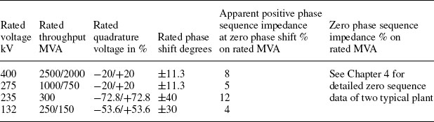
In this section, typical data and parameters for various power systems equipment is assembled and presented in tabular format. Throughout, the parameters used are defined as follows:
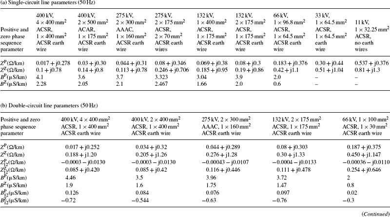
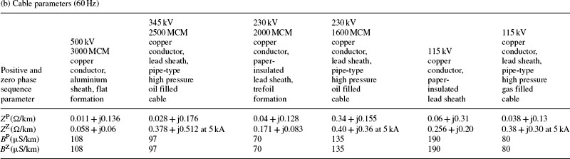
For overhead lines, cables, reactors and capacitors
ZP/RP/XP: positive phase sequence (PPS) impedance/resistance/reactance of a three-phase circuit
ZZ/RZ/XZ: zero phase sequence (ZPS) impedance/resistance/reactance of a three-phase circuit
BP/BZ: PPS/ZPS susceptance of a three-phase circuit
![]() : PPS/ZPS mutual impedance between two adjacent three-phase circuits
: PPS/ZPS mutual impedance between two adjacent three-phase circuits
![]() : PPS/ZPS mutual susceptance between two adjacent three-phase circuits
: PPS/ZPS mutual susceptance between two adjacent three-phase circuits
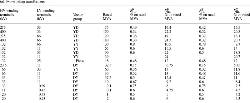
For transformers
Z/R/X is leakage impedance/resistance/reactance.
HL represents high voltage to low voltage leakage parameter, HT represents high voltage to low voltage leakage parameter and LT represents low voltage to tertiary voltage leakage parameter.
For synchronous machines
X″d/X′d/Xd: d-axis subtransient/transient/synchronous reactance and X″q is q-axis subtransient reactance. XZ is ZPS reactance and Ra is armature ac resistance
T″d/T′d: d-axis subtransient/transient short-circuit time constant
Ta: armature or dc short-circuit time constant. H is inertia constant.
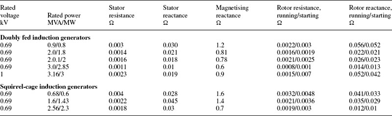
For induction machines
Double-cage or deep-bar: X″/X′/X is subtransient/transient/steady state reactance
T″/T′: subtransient/transient short-circuit time constant
Ta: armature or dc short-circuit time constant
Single-cage: X′/X is transient/steady state reactance