CHAPTER 17
Complexity Theory
An algorithm's performance is always important when you try to solve a problem. An algorithm won't do you much good if it takes too long or requires too much memory or other resources to actually run on a computer.
Computational complexity theory, or just complexity theory, is the closely related study of the difficulty of computational problems. Rather than focusing on specific algorithms, complexity theory focuses on problems.
For example, the mergesort algorithm described in Chapter 6 can sort a list of N numbers in O(N log N) time. Complexity theory asks what you can learn about the task of sorting in general, not what you can learn about a specific algorithm. It turns out you can show that any sorting algorithm that sorts by using comparisons must use at least N × log(N) time in the worst case.
N LOG N SORTING
To understand why any algorithm that uses comparisons to sort a list must use at least N log N time in the worst case, suppose you have an array of N unique items. Because they are unique, there are N! possible ways you can arrange them. To look at this in a different way, depending on what the values in the array are, there are N! ways the algorithm might need to rearrange the items to put them in sorted order. That means the algorithm must be able to follow N! possible paths of execution to produce every possible result.
The only tool the algorithm can use for branching into different paths of execution is to compare two values. So you can think of the possible paths of execution as a binary tree in which each node represents a comparison and each leaf node represents a final arrangement of the items in the array.
There are N! possible arrangements of the items in the array, so the execution tree must have N! leaf nodes. Because this is a binary tree, it has height log2(N!). Then log2(N!) = log2(N) + log2(N − 1) + log2(N − 2) +... + log2(2). Half of these terms (and that makes N ÷ 2 terms) are at least log2(N ÷ 2), so log2(N!)≥N ÷ 2 × log2(N ÷ 2), which is of the order N log N.
Complexity theory is a large and difficult topic, so there's no room here to cover it fully. However, every programmer who studies algorithms should know at least something about complexity theory in general and the two sets P and NP in particular. This chapter introduces complexity theory and describes what these important classes of problems are.
Notation
One of the first topics covered in this book was Big O notation. Chapter 1 described Big O notation somewhat intuitively by saying it describes how an algorithm's worst-case performance increases as the problem's size increases.
For most purposes, that definition is good enough to be useful, but in complexity theory Big O notation has a more technical definition. If an algorithm's run time is f(N), the algorithm has Big O performance of g(N) if f(N) < g(N) × k for some constant k and for N large enough. In other words, the function g(N) is an upper bound for the actual run time function f(N).
Two other notations similar to Big O notations are sometimes useful when discussing algorithmic complexity. Big Omega notation, written Ω(g(N)), means the run time function is bounded below by the function g(N). For example, as explained a moment ago, N log(N) is a lower bound for algorithms that sort by using comparisons, so those algorithms are Ω(N log N).
Big Theta notation, written Θ (g(N)), means the run time function is bounded both above and below by the function g(N). For example, the mergesort algorithm's run time is bounded above by O(N log N), and the run time of any algorithm that sorts by using comparisons is bounded below by Ω(N log N), so mergesort has performance Θ(N log N).
In summary, Big O notation gives an upper bound, Big Omega (Ω) gives a lower bound, and Big Theta (Θ) gives an upper and lower bound.
Note that some algorithms have different upper and lower bounds. For example, like all algorithms that sort by using comparisons, quicksort has a lower bound of Ω(N log N). In the best and expected cases, quicksort's performance actually is Ω(N log N). In the worst case, however, quicksort's performance is O(N2). The algorithm's lower and upper bounds are different, so no function gives quicksort a Big Theta notation. In practice, however, quicksort is often faster than algorithms such as mergesort that are tightly bounded by Θ(N log N), so it is still a popular algorithm.
Complexity Classes
Algorithmic problems are sometimes grouped into classes of algorithms that have similar run times (or space requirements) when running on a certain type of hypothetical computer.
The two most common kinds of hypothetical computers are deterministic and nondeterministic.
A deterministic computer's actions are completely determined by a finite set of internal states (the program's variables and code) and its input. In other words, if you feed a certain set of inputs into the computer, the results are completely predictable. (More technically, the “computer” used for this definition is a Turing machine fairly similar to the DFAs described in Chapter 15.)
TURING MACHINES
The concept of a Turing machine was invented by Alan Turing in 1936 (although he called it an “a-machine”). The idea was to make a conceptual machine that was extremely simple so that you could prove theorems about what such a machine could and could not compute.
A Turing machine is a simple finite automaton that uses a set of internal states that determine what the machine does as it reads its input. This is very similar to the DFAs and FNAs described in Chapter 15. The main difference is that the Turing machine's input is given as a string of 0s and 1s on a single-ended infinitely long tape that the machine can read from and write to. When the machine reads a 0 or 1 from the tape, the machine's states determine the following:
- Whether the machine should write a 0 or 1 onto the tape's current position
- Whether the machine's “read/write head” moves left, moves right, or stays in the same position on the tape
- The new state the machine should enter
Despite its simplicity, a Turing machine provides a fairly good model of actual computers, although creating a Turing machine to simulate a complicated program can be quite hard.
Turing machines have several variations. Some use a tape that is infinitely long in both directions. Others use multiple tapes and multiple read/write heads. Some are nondeterministic, so they can be in more than one state at the same time. Some allow null transitions so that the machine can move to a new state without reading anything.
One of the interesting results of studying Turing machines is that all these different kinds of machines have the same power. In other words, they can all perform the same computations.
For more information on Turing machines, see http://en.wikipedia.org/wiki/Turing_machine.
In contrast, a nondeterministic computer is allowed to be in multiple states at one time. This is similar to how the NFAs described in Chapter 15 can be in multiple states at once. Because the nondeterministic machine can follow any number of paths through its states to an accepting state, all it really needs to do is use the input on all the possible states it could be in and verify that one of the paths of execution works. Essentially (and less precisely), that means it can guess the correct solution and then simply verify that the solution is correct.
Note that a nondeterministic computer doesn't need to prove negative results. If there is a solution, the computer is allowed to guess the solution and verify it. If there is no solution, the computer doesn't need to prove that.
For example, to find the prime factors for an integer, a deterministic computer would need to somehow find the factors, perhaps by trying all possible factors up to the number's square root or by using a sieve of Eratosthenes. (See Chapter 2 for more information on those methods.) This would take a very long time.
In contrast, a nondeterministic computer can guess the factorization and then verify that it is correct by multiplying the factors together to see that the product is the original number. This would take very little time.
After you understand what the terms deterministic and nondeterministic mean in this context, understanding most of the common complexity classes is relatively easy. The following list summarizes the most important deterministic complexity classes:
- DTIME(f(N))—Problems that can be solved in f(N) time by a deterministic computer. These problems can be solved by some algorithm with run time O(f(N)) for some function f(N). For example, DTIME(N log N) includes problems that can be solved in O(N log N) time, such as sorting by using comparisons.
- P—Problems that can be solved in polynomial time by a deterministic computer. These problems can be solved by some algorithm with run time O(NP) for some power P no matter how large, even O(N1000).
- EXPTIME (or EXP)—Problems that can be solved in exponential time by a deterministic computer. These problems can be solved by some algorithm with run time O(2f(N)) for some polynomial function f(N).
The following list summarizes the most important nondeterministic complexity classes:
- NTIME(f(N))—Problems that can be solved in f(N) time by a deterministic computer. These problems can be solved by some algorithm with run time O(f(N)) for some function f(N). For example, NTIME(N2) includes problems in which an algorithm can guess the answer and verify that it is correct in O(N2) time.
- NP—Problems that can be solved in polynomial time by a nondeterministic computer. For these problems, an algorithm guesses the correct solution and verifies that it works in polynomial time O(NP) for some power P.
- NEXPTIME (or NEXP)—Problems that can be solved in exponential time by a nondeterministic computer. For these problems, an algorithm guesses the correct solution and verifies that it works in exponential time O(2f(N)) for some polynomial function f(N).
Similarly, you can define classes of problems that can be solved with different amounts of available space. These have the rather predictable names DSPACE(f(N)), PSPACE (polynomial space), EXPSPACE (exponential space), NPSPACE (nondeterministic polynomial space), and NEXPSPACE (nondeterministic exponential space).
Some relationships among these classes are known. For example, P ⊆ NP. (The ⊆ symbol means “is a subset of,” so this statement means “P is a subset of NP.”) To see why this is true, suppose a problem is in P. Then there is a deterministic algorithm that can find a solution to the problem in polynomial time. In that case, you can use the same algorithm to solve the problem with a nondeterministic computer. If the algorithm works—in other words, if the solution it finds must be correct—that trivially proves the solution is correct, so the nondeterministic algorithm works too.
Some of the other relationships are less obvious. For example, PSPACE = NSPACE, and EXPSPACE = NEXSPACE.
The most profound question in complexity theory is, does P equal NP? Many problems, such as sorting, are known to be in P. Many other problems, such as the knapsack and traveling salesman problems described in Chapter 12, are known to be in NP. The big question is, are the problems in NP also in P?
Lots of people have spent a huge amount of time trying to determine whether these two sets are the same. No one has discovered a polynomial time deterministic algorithm to solve the knapsack or traveling salesman problem, but that doesn't prove that no such algorithm is possible.
One way you can compare the difficulty of two algorithms is by reducing one to the other, as described in the next section.
Reductions
To reduce one problem to another, you must come up with a way for the solution to one problem to give you the solution to the other. If you can do that within a certain amount of time, the maximum run time of the two algorithms is the same within the amount of time you spent on the reduction.
For example, you know that prime factoring is in NP and that sorting is in P. Suppose you could find an algorithm that can reduce factoring into a sorting problem, and the reduction takes only polynomial time. In that case, you could solve factoring problems in polynomial time by solving the corresponding sorting problem. (Of course, no one knows how to reduce factoring to sorting. If someone had discovered such a reduction, factoring wouldn't be as hard as it is.)
Polynomial time reductions are particularly important because they let you reduce many problems in NP to other problems in NP. In fact, there are some problems to which every problem in NP can be reduced. Those problems are called NP-complete.
The first known NP-complete problem was the satisfiability problem (SAT). In this problem, you are given a boolean expression that includes variables that could be true or false, such as (A AND B) OR (B AND NOT C). The goal is to determine whether there is a way to assign the values true and false to the variables to make the statement true.
The Cook-Levin theorem (or just Cook's theorem) proves that SAT is NP-complete. The details are rather technical (see http://en.wikipedia.org/wiki/Cook-Levin_theorem for details), but the basic ideas aren't too confusing.
To show that SAT is NP-complete, you need to do two things: Show that SAT is in NP, and show that any other problem in NP can be reduced to SAT.
SAT is in NP because you can guess the assignments for the variables and then verify that those assignments make the statement true.
Proving that any other problem in NP can be reduced to SAT is the tricky part. Suppose a problem is in NP. In that case, you must be able to make a nondeterministic Turing machine with internal states that let it solve the problem. The idea behind the proof is to build a boolean expression that says the inputs are passed into the Turing machine, the states work correctly, and the machine stops in an accepting state.
The boolean expression contains three kinds of variables that are named Tijk, Hik, and Qqk for various values of i, j, k, and q. The following list explains each variable's meaning:
- Tijk is true if tape cell i contains symbol j at step k of the computation.
- Hik is true if the machine's read/write head is on tape cell i at step k of the computation.
- Qqk is true if the machine is in state q at step k of the computation.
The expression must also include some terms to represent how a Turing machine works. For example, suppose the tape can hold only 0s and 1s. Then the statement (T001 AND NOT T011) OR (NOT T001 AND T011) means that cell 0 at step 1 of the computation contains either a 0 or a 1 but not both.
Other parts of the expression ensure that the read/write head is in a single position at each step of the computation, that the machine starts in state 0, that the read/write head starts at tape cell 0, and so on.
The full boolean expression is equivalent to the original Turing machine for the problem in NP. In other words, if you set the values of the variables Tijk to represent a series of inputs, the truth of the boolean expression tells you whether the original Turing machine would accept those inputs.
This reduces the original problem to the problem of determining whether the boolean expression can be satisfied so that SAT is NP-complete.
Once you have found one problem that is NP-complete, such as SAT, you can prove that other problems are NP-complete by reducing them to the first problem.
If problem A and B can be reduced to problem B in polynomial time, you can write A ≤p B.
The following sections provide examples that reduce one problem to another.
3SAT
The 3SAT problem is to determine whether a boolean expression in three-term conjunctive normal form can be satisfied. Three-term conjunctive normal form (3CNF) means that the boolean expression consists of a series of clauses combined with AND and NOT, and that each clause combines exactly three variables with OR and NOT. For example, the following statements are all in 3CNF:
- (A OR B OR NOT C) AND (C OR NOT A OR B)
- (A OR C OR C) AND (A OR B OR B)
- (NOT A OR NOT B OR NOT C)
Clearly 3SAT is in NP because, as is the case with SAT, you can guess an assignment of true and false to the variables and then check whether the statement is true.
With some work, you can convert any boolean expression in polynomial time into an equivalent expression in 3CNF. That means SAT is polynomial-time reducible to SAT. Because SAT is NP-complete, 3SAT must also be NP-complete.
Bipartite Matching
A bipartite graph is one in which the nodes are divided into two sets and no link connects two nodes in the same set, as shown in Figure 17-1.
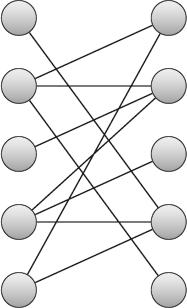
Figure 17-1: In a bipartite graph, the nodes are divided into two sets, and links can only connect nodes in one set to nodes in the other.
In the bipartite graph, a matching is a set of links, no two of which share a common end point..
In the bipartite matching problem, given a bipartite graph and a number k, is there a matching that contains at least k links?
The section “Work Assignment” in Chapter 14 explained how you could use a maximal flow problem to perform work assignment. Work assignment is simply a bipartite matching between nodes representing employees and nodes representing jobs, so that algorithm also solves the bipartite matching problem.
Add a source node, and connect it to all the nodes in one set. Create a sink node, and connect all the nodes in the other set to it. Now the maximal flow algorithm finds a maximal bipartite matching. After you find the matching, compare the maximal flow to the number k.
NP-Hardness
A problem is NP-complete if it is in NP and every other problem in NP is polynomial-time reducible to it. A problem is NP-hard if every other problem in NP is polynomial-time reducible to it. The only difference between NP-complete and NP-hard is that an NP-hard problem need not be in NP.
Note that all NP-complete problems are NP-hard, plus they are in NP.
Being NP-hard in some sense means the problem is at least as hard as any problem in NP, because you can reduce any problem in NP to it.
You can show that a problem is NP-complete by showing it is polynomial-time reducible to an NP-complete problem. Similarly, you can show that a problem is NP-hard by showing it is polynomial-time reducible to an NP-hard problem.
Detection, Reporting, and Optimization Problems
Many interesting problems come in three forms: detection, reporting, and optimization. The detection problem asks if a solution of a given quality exists. The reporting problem asks you to find a solution of a given quality. The optimization problem asks you to find the best possible solution.
For example, in the subset sum problem, you are given a set of numbers, and there are three associated problems:
- Detection—Is there a subset of the numbers that adds up to a specific value k?
- Reporting—Find a subset of the numbers that adds up to the specific value k, if such a subset exists.
- Optimization—Find a subset of the numbers with a total as close to the specific value k as possible.
(A variation on the subset sum problem asks you to find a subset with values that total 0.)
At first some of these problems may seem easier than others. For example, the detection problem only asks you to prove that a subset adds up to 0. Because it doesn't make you find subsets like the reporting problem does, you might think the detection problem is easier. In fact, you can use reductions to show that the three forms of problems have the same difficulty, at least as far as complexity theory is concerned.
To do that, you need to show four reductions:
- Detection ≤p Reporting
- Reporting ≤p Optimization
- Reporting ≤p Detection
- Optimization ≤p Reporting
Reductions are transitive, so the first two reductions show that Detection ≤p Reporting ≤p Optimization, and the second two reductions show that Optimization p ≤p Reporting ≤p Detection.
Detection ≤p Reporting
The reduction Detection ≤p Reporting is relatively obvious. If you have an algorithm for reporting subsets, you can use it to detect subsets. For a value k, use the reporting algorithm to find a subset that adds up to k. If the algorithm finds one, the answer to the detection problem is, “Yes, such a subset exists.”
For a specific example, suppose ReportSum is a reporting algorithm for the subset sum problem. In other words, ReportSum(k) returns a subset with sum k if such a subset exists. Then DetectSum(k) can simply call ReportSum(k) and return true if ReportSum(k) returns a subset.
Reporting ≤p Optimization
The reduction Reporting ≤p Optimization also is fairly obvious. Suppose you have an algorithm for finding the optimal solution. Then use it to find an optimal solution. If that solution is within the value k specified by the reporting problem, the reporting problem can return the solution found by the optimization algorithm. If the solution found by the optimization problem is not within the value k, the reporting algorithm should return false.
For a specific example, suppose OptimizeSum(k) returns a subset with a total as close as possible to the value k. Then ReportSum(k) can call OptimizeSum(k) and see if the returned subset's total is k. If the total is k, ReportSum(k) returns that subset. If the total is not k, ReportSum(k) returns nothing to indicate that no such subset exists.
Reporting ≤p Detection
The reduction Reporting ≤p Detection is less obvious than the previous reductions. First, use the detection algorithm to see if a solution is possible. If there is no solution, the reporting algorithm doesn't need to do anything.
If a solution is possible, simplify the problem somehow to give an equivalent problem, and then use the detection algorithm to see if a solution is still possible. If a solution no longer exists, remove the simplification, and try a different one. When you have tried all possible simplifications, and none of them will work, whatever is left must be the solution that the reporting algorithm should return.
For a specific example, suppose DetectSum(k) returns true if there is a subset with a total value equal to k. The following pseudocode shows how to use that algorithm to build a ReportSum algorithm:
- Use DetectSum(k) on the whole set to see if a solution is possible. If no solution is possible, the ReportSum algorithm returns that fact and is done.
- For each value Vi in the set:
- Remove Vi from the set, and call DetectSum(k) for the remaining set to see if there is still a subset with total value k.
- If DetectSum(k) returns false, restore Vi to the set, and continue the loop at Step 2.
- If DetectSum(k) returns true, leave Vi out of the set, and continue the loop at Step 2.
When the loop in Step 2 finishes, the remaining values in the set form a subset with total value k.
Optimization ≤p Reporting
The final step in showing that the three kinds of problems have the same complexity is showing that Optimization ≤p Reporting. Suppose you have a reporting algorithm Report(k). Then the optimization algorithm can call Report(k), Report(k + 1), Report(k + 2), and so on until it finds a solution. (If the problem also allows solutions of the form Report(k − 1), try those too.)
For a specific example, suppose ReportSum(k) returns a subset with total value k if one exists. Then the following steps describe an algorithm for OptimizeSum(k):
- For i = 0 To N, where N is the number of items in the set:
- If ReportSum(k + i) returns a subset, OptimizeSum should return that subset.
- If ReportSum(k − i) returns a subset, OptimizeSum should return that subset.
- Continue the loop in Step 1.
These reductions show Detection ≤p Reporting ≤p Optimization and Optimization ≤p Reporting ≤p Detection, so the problems all have the same complexity.
NP-Complete Problems
More than 3,000 NP-complete problems have been discovered, so the following list is only a very small subset of them. They are listed here to give you an idea of some kinds of problems that are NP-complete.
Remember that NP-complete problems have no known polynomial time solution, so these are all considered very hard problems. Many can only be solved exactly for very small problem sizes.
Because these problems are all NP-complete, there is a way to reduce each of them to every other problem:
- Art gallery problem—Given an arrangement of rooms and hallways in an art gallery, find the minimum number of guards needed to watch the entire gallery.
- Bin packing—Given a set of objects and a series of bins, find a way to pack the objects into the bins to use the fewest bins possible.
- Bottleneck traveling salesman problem—Find a Hamiltonian path through a weighted network that has the minimum possible largest link weight.
- Chinese postman problem (or route inspection problem)—Given a network, find the shortest circuit that visits every link.
- Chromatic number (or vertex coloring)—Given a graph, find the smallest number of colors needed to color the graph's nodes. (The graph is not necessarily planar.)
- Clique—Given a graph, find the largest clique in the graph. (A clique is a set of nodes that are all mutually connected. In other words, every pair of nodes in the set has an edge connecting the pair of nodes.)
- Clique cover problem—Given a graph and a number k, find a way to partition the graph into k sets that are all cliques.
- Degree-constrained spanning tree—Given a graph, find a spanning tree with a given maximum degree.
- Dominating set—Given a graph, find a set of nodes S so that every other node is adjacent to one of the nodes in the set S.
- Feedback vertex set—Given a graph, find the smallest set S of vertices that you can remove to leave the graph free of cycles.
- Hamiltonian completion—Find the minimum number of edges you need to add to a graph to make it Hamiltonian (in other words, to make it so that it contains a Hamiltonian path).
- Hamiltonian cycle—Determine whether there is a path through a graph that visits every node exactly once and then returns to its starting point.
- Hamiltonian path (HAM)—Determine whether there is a path through a graph that visits every node exactly once.
- Job shop scheduling—Given N jobs of various sizes and M identical machines, schedule the jobs for the machines to minimize the total time to finish all the jobs.
- Knapsack—Given a knapsack with a given capacity and a set of objects with weights and values, find the set of objects with the largest possible weight that fits in the knapsack.
- Longest path—Given a network, find the longest path that doesn't visit the same node twice.
- Maximum independent set—Given a graph, find the largest set of nodes where no two nodes in the set are connected by a link.
- Maximum leaf spanning tree—Given a graph, find a spanning tree that has the maximum possible number of leaves.
- Minimum degree spanning tree—Given a graph, find a spanning tree with the minimum possible degree.
- Minimum k-cut—Given a graph and a number k, find the minimum weight set of edges that you can remove to divide the graph into k pieces.
- Partitioning—Given a set of integers, find a way to divide the values into two sets with the same total value. (Variations use more than two sets.)
- Satisfiability (SAT)—Given a boolean expression containing variables, find an assignment of true and false to the variables to make the expression true. (See the earlier section “Reductions” for more details.)
- Shortest path—Given a (not necessarily planar) network, find the shortest path between two given nodes.
- Subset sum—Given a set of integers, find a subset with a given total value.
- Three-partition problem—Given a set of integers, find a way to divide the set into triples that all have the same total value.
- Three-satisfiability (3SAT)—Given a boolean expression in conjunctive normal form, find an assignment of true and false to the variables to make the expression true. (See the earlier section “3SAT” for more details.)
- Traveling salesman problem (TSP)—Given a list of cities and the distances between them, find the shortest possible route that visits all the cities and returns to the starting city.
- Unbounded knapsack—Similar to the knapsack problem, except that you can select any item multiple times.
- Vehicle routing—Given a set of customer locations and a fleet of vehicles, find the most efficient routes for the vehicles to visit all the customer locations. (This problem has many variations. For example, the route might require delivery only or both pickup and delivery, items might need to be delivered in last-picked-up-next-delivered order, vehicles might have differing capacities, and so on.)
- Vertex cover—Given a graph, find a minimal set of vertices so that every link in the graph touches one of the selected vertices.
Summary
This chapter provided a brief introduction to complexity theory. It explained what complexity classes are and described some of the more important ones, including P and NP. You don't necessarily need to know the fine details of every complexity class, but you should certainly understand P and NP. You should also be familiar with perhaps the most profound question in computer science: Does P equal NP?
Later sections in this chapter explained how to use polynomial time reductions to show that one problem is at least as hard as another. Those sorts of reductions are useful for studying complexity theory, but the concept of reducing one problem to another is also useful more generally for using an existing solution to solve a new problem. This chapter doesn't describe any practical algorithm you might want to implement on a computer, but the reductions show how you can use an algorithm that solves one problem to solve a different problem.
The problems described in this chapter may also help you realize when you're attempting to solve a very hard problem, so that you'll know a perfect solution may be impossible. If you face a programming problem that is another version of the Hamiltonian path, traveling salesman, or knapsack problem, you know you can only solve the problem exactly for small problem sizes.
Chapter 12 discusses methods you can use to address some of these very hard problems. Branch and bound lets you solve problems that are larger than you could otherwise solve by using a brute-force approach. Heuristics let you find approximate solutions to even larger problems.
Another technique that lets you address larger problems is parallelism. If you can divide the work across multiple CPUs or computers, you may be able to find problems that would be impractical on a single computer. The next chapter describes some algorithms that are useful when you can use multiple CPUs or computers to solve a problem.
Exercises
Asterisks indicate particularly difficult problems.
- If any algorithm that sorts by using comparisons must use at least O(N log N) time in the worst case, how do algorithms such as the countingsort and bucketsort algorithms described in Chapter 6 sort more quickly than that?
- The bipartite detection problem is as follows: Given a graph, is the graph bipartite? Find a polynomial time reduction of this problem to a map coloring problem. What can you conclude about the complexity class containing bipartite detection?
- The three-cycle problem is as follows: Given a graph, does the graph contain any cycles of length 3? Find a polynomial time reduction of this problem to another problem. What can you conclude about the complexity class containing the three-cycle problem?
- The odd-cycle problem is as follows: Given a graph, does the graph contain any cycles of odd length? Find a polynomial time reduction of this problem to another problem. What can you conclude about the complexity class containing the odd-cycle problem? How does this relate to the three-cycle problem?
- The Hamiltonian path problem (HAM) is as follows: Given a network, is there a path that visits every node exactly once? Show that HAM is in NP.
- The Hamiltonian cycle or Hamiltonian circuit problem (call it HAMC) is as follows: Given a network, is there a path that visits every node exactly once and returns to its starting node? Show that this problem is in NP.
- **Find a polynomial time reduction of HAM to HAMC.
- **Find a polynomial time reduction of HAMC to HAM.
- The network coloring problem is as follows: Given a network and a number k, is there a way to k-color the network's nodes? Show that this problem is in NP.
- The zero sum subset problem is as follows: Given a set of numbers, does a subset of the numbers add up to 0? Show that this problem is in NP.
- *Suppose you are given a set of objects with weights Wi and values Vi, and a knapsack that can hold a total weight of W. Then three forms of the knapsack problem are as follows:
- Detection—For a value k, is there a subset of objects that fit into the knapsack and have a total value of at least k?
- Reporting—For a value k, find a subset of objects that fit into the knapsack and have a total value of at least k if such a subset exists.
- Optimization—Find a subset that fits in the knapsack with the largest possible total value.
Find a reduction of the reporting problem to the detection problem.
- *For the problems defined in Exercise 11, find a reduction of the optimization problem to the detection problem.
- **Suppose you are given a set of objects with values Vi. Then two forms of the partition problem are as follows:
- Detection—Is there a way to divide the objects into two subsets A and B that have the same total value?
- Reporting—Find a way to divide the objects into two subsets A and B that have the same total value.
Find a reduction of the reporting problem to the detection problem.