2
Location and Simple Linear Models
In statistical literature, various methods of estimation of the parameters of a given model are available, primarily based on the least squares estimator (LSE) and maximum likelihood estimator (MLE) principle. However, when uncertain prior information of the parameters is known, the estimation technique changes. The methods of circumvention, including the uncertain prior information, are of immense importance in the current statistical literature. In the area of classical approach, preliminary test (PT) and the Stein‐type (S) estimation methods dominate the modern statistical literature, side by side with the Bayesian methods.
In this chapter, we consider the simple linear model and the estimation of the parameters of the model along with their shrinkage version and study their properties when the errors are normally distributed.
2.1 Introduction
Consider the simple linear model with slope ![]() and intercept
and intercept ![]() , given by
, given by
If ![]() , the model (2.1) reduces to
, the model (2.1) reduces to
where ![]() is the location parameter of a distribution.
is the location parameter of a distribution.
In the following sections, we consider the estimation and test of the location model, i.e. the model of (2.2), followed by the estimation and test of the simple linear model.
2.2 Location Model
In this section, we introduce two basic penalty estimators, namely, the ridge regression estimator (RRE) and the least absolute shrinkage and selection operator (LASSO) estimator for the location parameter of a distribution. The penalty estimators have become viral in statistical literature. The subject evolved as the solution to ill‐posed problems raised by Tikhonov (1963) in mathematics. In 1970, Hoerl and Kennard applied the Tikhonov method of solution to obtain the RRE for linear models. Further, we compare the estimators with the LSE in terms of ![]() ‐risk function.
‐risk function.
2.2.1 Location Model: Estimation
Consider the simple location model,
where ![]() ,
, ![]() ‐
‐ ![]() ‐tuple of 1's, and
‐tuple of 1's, and ![]()
![]() ‐vector of i.i.d. random errors such that
‐vector of i.i.d. random errors such that ![]() and
and ![]() ,
, ![]() is the identity matrix of rank
is the identity matrix of rank ![]() (
(![]() ),
), ![]() is the location parameter, and, in this case,
is the location parameter, and, in this case, ![]() may be unknown.
may be unknown.
The LSE of ![]() is obtained by
is obtained by
Alternatively, it is possible to minimize the log‐likelihood function when the errors are normally distributed:
giving the same solution (2.4) as in the case of LSE. It is known that the ![]() is unbiased, i.e.
is unbiased, i.e. ![]() and the variance of
and the variance of ![]() is given by
is given by
The unbiased estimator of ![]() is given by
is given by
The mean squared error (MSE) of ![]() , any estimator of
, any estimator of ![]() , is defined as
, is defined as
Test for ![]() when
when ![]() is known:
is known:
For the test of null‐hypothesis ![]() vs.
vs. ![]() , we use the test statistic
, we use the test statistic
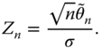
Under the assumption of normality of the errors, ![]() , where
, where ![]() Hence, we reject
Hence, we reject ![]() whenever
whenever ![]() exceeds the threshold value from the null distribution. An interesting threshold value is
exceeds the threshold value from the null distribution. An interesting threshold value is ![]() .
.
For large samples, when the distribution of errors has zero mean and finite variance ![]() , under a sequence of local alternatives,
, under a sequence of local alternatives,
and assuming ![]() and
and ![]() (
(![]() ),
), ![]() , the asymptotic distribution of
, the asymptotic distribution of ![]() is
is ![]() . Then the test procedure remains the same as before.
. Then the test procedure remains the same as before.
2.2.2 Shrinkage Estimation of Location
In this section, we consider a shrinkage estimator of the location parameter ![]() of the form
of the form
where ![]() . The bias and the MSE of
. The bias and the MSE of ![]() are given by
are given by

Minimizing ![]() w.r.t.
w.r.t. ![]() , we obtain
, we obtain
So that
Thus, ![]() is an increasing function of
is an increasing function of ![]() and the relative efficiency (REff) of
and the relative efficiency (REff) of ![]() compared to
compared to ![]() is
is
Further, the MSE difference is
Hence, ![]() outperforms the
outperforms the ![]() uniformly.
uniformly.
2.2.3 Ridge Regression–Type Estimation of Location Parameter
Consider the problem of estimating ![]() when one suspects that
when one suspects that ![]() may be 0. Then following Hoerl and Kennard (1970), if we define
may be 0. Then following Hoerl and Kennard (1970), if we define
Then, we obtain the ridge regression–type estimate of ![]() as
as
or

Note that it is the same as taking ![]() in (2.8).
in (2.8).
Hence, the bias and MSE of ![]() are given by
are given by
and

It may be seen that the optimum value of ![]() is
is ![]() and MSE at (2.18) equals
and MSE at (2.18) equals

Further, the MSE difference equals
which shows ![]() uniformly dominates
uniformly dominates ![]() .
.
The REff of ![]() is given by
is given by
2.2.4 LASSO for Location Parameter
In this section, we define the LASSO estimator of ![]() introduced by Tibshirani (1996) in connection with the regression model.
introduced by Tibshirani (1996) in connection with the regression model.
Donoho and Johnstone (1994) defined this estimator as the “soft threshold estimator” (STE).
2.2.5 Bias and MSE Expression for the LASSO of Location Parameter
In order to derive the bias and MSE of LASSO estimators, we need the following lemma.
Using Lemma 2.1, we can find the bias and MSE expressions of ![]() .
.
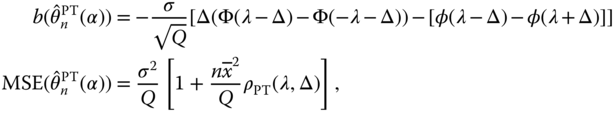
2.2.6 Preliminary Test Estimator, Bias, and MSE
Based on Saleh (2006), the preliminary test estimators (PTEs) of ![]() under normality assumption of the errors are given by
under normality assumption of the errors are given by

Thus, we have the following theorem about bias and MSE.
2.2.7 Stein‐Type Estimation of Location Parameter
The PT heavily depends on the critical value of the test that ![]() may be zero. Thus, due to down effect of discreteness of the PTE, we define the Stein‐type estimator of
may be zero. Thus, due to down effect of discreteness of the PTE, we define the Stein‐type estimator of ![]() as given here assuming
as given here assuming ![]() is known
is known

The bias of ![]() is
is ![]() , and the MSE of
, and the MSE of ![]() is given by
is given by

The value of ![]() that minimizes
that minimizes ![]() is
is ![]() , which is a decreasing function of
, which is a decreasing function of ![]() with a maximum at
with a maximum at ![]() and maximum value
and maximum value ![]() . Hence, the optimum value of MSE is
. Hence, the optimum value of MSE is
The REff compared to LSE, ![]() is
is
In general, the ![]() decreases from
decreases from ![]() at
at ![]() , then it crosses the 1‐line at
, then it crosses the 1‐line at ![]() , and for
, and for ![]() ,
, ![]() performs better than
performs better than ![]() .
.
2.2.8 Comparison of LSE, PTE, Ridge, SE, and LASSO
We know the following MSE from previous sections:

Hence, the REff expressions are given by

Table 2.1 Table of relative efficiency.
| 0.000 | 1.000 | 4.184 | 2.752 | 9.932 | |
| 0.316 | 1.000 | 11.000 | 2.647 | 2.350 | 5.694 |
| 0.548 | 1.000 | 4.333 | 1.769 | 1.849 | 3.138 |
| 0.707 | 1.000 | 3.000 | 1.398 | 1.550 | 2.207 |
| 1.000 | 1.000 | 2.000 | 1.012 | 1.157 | 1.326 |
| 1.177 | 1.000 | 1.721 | 0.884 | 1.000 | 1.046 |
| 1.414 | 1.000 | 1.500 | 0.785 | 0.856 | 0.814 |
| 2.236 | 1.000 | 1.200 | 0.750 | 0.653 | 0.503 |
| 3.162 | 1.000 | 1.100 | 0.908 | 0.614 | 0.430 |
| 3.873 | 1.000 | 1.067 | 0.980 | 0.611 | 0.421 |
| 4.472 | 1.000 | 1.050 | 0.996 | 0.611 | 0.419 |
| 5.000 | 1.000 | 1.040 | 0.999 | 0.611 | 0.419 |
| 5.477 | 1.000 | 1.033 | 1.000 | 0.611 | 0.419 |
| 6.325 | 1.000 | 1.025 | 1.000 | 0.611 | 0.419 |
| 7.071 | 1.000 | 1.020 | 1.000 | 0.611 | 0.419 |
It is seen from Table 2.1 that the RRE dominates all other estimators uniformly and LASSO dominates UE, PTE, and ![]() in an interval near 0. From Table 2.1, we find
in an interval near 0. From Table 2.1, we find ![]() in the interval
in the interval ![]() while outside this interval
while outside this interval ![]() . Figure 2.1 confirms that.
. Figure 2.1 confirms that.

Figure 2.1 Relative efficiencies of the estimators.
2.3 Simple Linear Model
In this section, we consider the model (2.1) and define the PT, ridge, and LASSO‐type estimators when it is suspected that the slope may be zero.
2.3.1 Estimation of the Intercept and Slope Parameters
First, we consider the LSE of the parameters. Using the model (2.1) and the sample information from the normal distribution, we obtain the LSEs of ![]() as
as

where
The exact distribution of ![]() is a bivariate normal with mean
is a bivariate normal with mean ![]() and covariance matrix
and covariance matrix

An unbiased estimator of the variance ![]() is given by
is given by
which is independent of ![]() , and
, and ![]() follows a central chi‐square distribution with
follows a central chi‐square distribution with ![]() degrees of freedom (DF)
degrees of freedom (DF)
2.3.2 Test for Slope Parameter
Suppose that we want to test the null‐hypothesis ![]() vs.
vs. ![]() . Then, we use the likelihood ratio (LR) test statistic
. Then, we use the likelihood ratio (LR) test statistic

where ![]() follows a noncentral chi‐square distribution with 1 DF and noncentrality parameter
follows a noncentral chi‐square distribution with 1 DF and noncentrality parameter ![]() and
and ![]() follows a noncentral
follows a noncentral ![]() ‐distribution with
‐distribution with ![]() , where
, where ![]() is DF and also the noncentral parameter is
is DF and also the noncentral parameter is

Under ![]() ,
, ![]() follows a central chi‐square distribution and
follows a central chi‐square distribution and ![]() follows a central
follows a central ![]() ‐distribution. At the
‐distribution. At the ![]() ‐level of significance, we obtain the critical value
‐level of significance, we obtain the critical value ![]() or
or ![]() from the distribution and reject
from the distribution and reject ![]() if
if ![]() or
or ![]() ; otherwise, we accept
; otherwise, we accept ![]() .
.
2.3.3 PTE of the Intercept and Slope Parameters
This section deals with the problem of estimation of the intercept and slope parameters ![]() when it is suspected that the slope parameter
when it is suspected that the slope parameter ![]() may be
may be ![]() .
.
From (2.30), we know that the LSE of ![]() is given by
is given by
If we know ![]() to be
to be ![]() exactly, then the restricted least squares estimator (RLSE) of
exactly, then the restricted least squares estimator (RLSE) of ![]() is given by
is given by
In practice, the prior information that ![]() is uncertain. The doubt regarding this prior information can be removed using Fisher's recipe of testing the null‐hypothesis
is uncertain. The doubt regarding this prior information can be removed using Fisher's recipe of testing the null‐hypothesis ![]() against the alternative
against the alternative ![]() . As a result of this test, we choose
. As a result of this test, we choose ![]() or
or ![]() based on the rejection or acceptance of
based on the rejection or acceptance of ![]() . Accordingly, in case of the unknown variance, we write the estimator as
. Accordingly, in case of the unknown variance, we write the estimator as
called the PTE, where ![]() is the
is the ![]() ‐level upper critical value of a central
‐level upper critical value of a central ![]() ‐distribution with
‐distribution with ![]() DF and
DF and ![]() is the indicator function of the set
is the indicator function of the set ![]() . For more details on PTE, see Saleh (2006), Ahmed and Saleh (1988), Ahsanullah and Saleh (1972), Kibria and Saleh (2012) and, recently Saleh et al. (2014), among others. We can write PTE of
. For more details on PTE, see Saleh (2006), Ahmed and Saleh (1988), Ahsanullah and Saleh (1972), Kibria and Saleh (2012) and, recently Saleh et al. (2014), among others. We can write PTE of ![]() as
as
If ![]() ,
, ![]() is always chosen; and if
is always chosen; and if ![]() ,
, ![]() is chosen. Since
is chosen. Since ![]() ,
, ![]() in repeated samples, this will result in a combination of
in repeated samples, this will result in a combination of ![]() and
and ![]() . Note that the PTE procedure leads to the choice of one of the two values, namely, either
. Note that the PTE procedure leads to the choice of one of the two values, namely, either ![]() or
or ![]() . Also, the PTE procedure depends on the level of significance
. Also, the PTE procedure depends on the level of significance ![]() .
.
Clearly, ![]() is the unrestricted estimator of
is the unrestricted estimator of ![]() , while
, while ![]() is the restricted estimator. Thus, the PTE of
is the restricted estimator. Thus, the PTE of ![]() is given by
is given by
Now, if ![]() ,
, ![]() is always chosen; and if
is always chosen; and if ![]() ,
, ![]() is always chosen.
is always chosen.
Since our interest is to compare the LSE, RLSE, and PTE of ![]() and
and ![]() with respect to bias and the MSE, we obtain the expression of these quantities in the following theorem. First we consider the bias expressions of the estimators.
with respect to bias and the MSE, we obtain the expression of these quantities in the following theorem. First we consider the bias expressions of the estimators.
Next, we consider the expressions for the MSEs of ![]() ,
, ![]() , and
, and ![]() along with the
along with the ![]() ,
, ![]() , and
, and ![]() .
.
2.3.4 Comparison of Bias and MSE Functions
Since the bias and MSE expressions are known to us, we may compare them for the three estimators, namely, ![]() ,
, ![]() , and
, and ![]() as well as
as well as ![]() ,
, ![]() , and
, and ![]() . Note that all the expressions are functions of
. Note that all the expressions are functions of ![]() , which is the noncentrality parameter of the noncentral
, which is the noncentrality parameter of the noncentral ![]() ‐distribution. Also,
‐distribution. Also, ![]() is the standardized distance between
is the standardized distance between ![]() and
and ![]() . First, we compare the bias functions as in Theorem 2.4, when
. First, we compare the bias functions as in Theorem 2.4, when ![]() is unknown.
is unknown.
For ![]() or under
or under ![]() ,
,

Otherwise, for all ![]() and
and ![]() ,
,

The absolute bias of ![]() is linear in
is linear in ![]() , while the absolute bias of
, while the absolute bias of ![]() increases to the maximum as
increases to the maximum as ![]() moves away from the origin, and then decreases toward zero as
moves away from the origin, and then decreases toward zero as ![]() . Similar conclusions hold for
. Similar conclusions hold for ![]() .
.
Now, we compare the MSE functions of the restricted estimators and PTEs with respect to the traditional estimator, ![]() and
and ![]() , respectively. The REff of
, respectively. The REff of ![]() compared to
compared to ![]() may be written as
may be written as

The efficiency is a decreasing function of ![]() . Under
. Under ![]() (i.e.
(i.e. ![]() ), it has the maximum value
), it has the maximum value

and ![]() , accordingly, as
, accordingly, as ![]() . Thus,
. Thus, ![]() performs better than
performs better than ![]() whenever
whenever ![]() ; otherwise,
; otherwise, ![]() performs better
performs better ![]() .
.
The REff of ![]() compared to
compared to ![]() may be written as
may be written as
where

Under the ![]() , it has the maximum value
, it has the maximum value

and ![]() according as
according as

Hence, ![]() performs better than
performs better than ![]() if
if ![]() ; otherwise,
; otherwise, ![]() is better than
is better than ![]() . Since
. Since
we obtain

Figure 2.2 Graph of  and
and  for
for  and
and  .
.
As for the PTE of ![]() , it is better than
, it is better than ![]() , if
, if

Otherwise, ![]() is better than
is better than ![]() . The
. The

Under ![]() ,
,
See Figure 2.2 for visual comparison between estimators.
2.3.5 Alternative PTE
In this subsection, we provide the alternative expressions for the estimator of PT and its bias and MSE. To test the hypothesis ![]() vs.
vs. ![]() , we use the following test statistic:
, we use the following test statistic:

The PTE of ![]() is given by
is given by

where ![]() .
.
Hence, the bias of ![]() equals
equals ![]() , and the MSE is given by
, and the MSE is given by

Next, we consider the Stein‐type estimator of ![]() as
as

The bias and MSE expressions are given respectively by

As a consequence, we may define the PT and Stein‐type estimators of ![]() given by
given by

Then, the bias and MSE expressions of ![]() are
are
where

Similarly, the bias and MSE expressions for ![]() are given by
are given by

2.3.6 Optimum Level of Significance of Preliminary Test
Consider the REff of ![]() compared to
compared to ![]() . Denoting it by
. Denoting it by ![]() , we have
, we have
where

The graph of ![]() , as a function of
, as a function of ![]() for fixed
for fixed ![]() , is decreasing crossing the 1‐line to a minimum at
, is decreasing crossing the 1‐line to a minimum at ![]() (say); then it increases toward the 1‐line as
(say); then it increases toward the 1‐line as ![]() . The maximum value of
. The maximum value of ![]() occurs at
occurs at ![]() with the value
with the value

for all ![]() , the set of possible values of
, the set of possible values of ![]() . The value of
. The value of ![]() decreases as
decreases as ![]() ‐values increase. On the other hand, if
‐values increase. On the other hand, if ![]() and
and ![]() vary, the graphs of
vary, the graphs of ![]() and
and ![]() intersect at
intersect at ![]() . In general,
. In general, ![]() and
and ![]() intersect within the interval
intersect within the interval ![]() ; the value of
; the value of ![]() at the intersection increases as
at the intersection increases as ![]() ‐values increase. Therefore, for two different
‐values increase. Therefore, for two different ![]() ‐values,
‐values, ![]() and
and ![]() will always intersect below the 1‐line.
will always intersect below the 1‐line.
In order to obtain a PTE with a minimum guaranteed efficiency, ![]() , we adopt the following procedure: If
, we adopt the following procedure: If ![]() , we always choose
, we always choose ![]() , since
, since ![]() in this interval. However, since in general
in this interval. However, since in general ![]() is unknown, there is no way to choose an estimate that is uniformly best. For this reason, we select an estimator with minimum guaranteed efficiency, such as
is unknown, there is no way to choose an estimate that is uniformly best. For this reason, we select an estimator with minimum guaranteed efficiency, such as ![]() , and look for a suitable
, and look for a suitable ![]() from the set,
from the set, ![]() . The estimator chosen maximizes
. The estimator chosen maximizes ![]() over all
over all ![]() and
and ![]() . Thus, we solve the following equation for the optimum
. Thus, we solve the following equation for the optimum ![]() :
:
The solution ![]() obtained this way gives the PTE with minimum guaranteed efficiency
obtained this way gives the PTE with minimum guaranteed efficiency ![]() , which may increase toward
, which may increase toward ![]() given by (2.61), and Table 2.2. For the following given data, we have computed the maximum and minimum guaranteed REff for the estimators of
given by (2.61), and Table 2.2. For the following given data, we have computed the maximum and minimum guaranteed REff for the estimators of ![]() and provided them in Table 2.2.
and provided them in Table 2.2.

Table 2.2 Maximum and minimum guaranteed relative efficiency.
| 0.05 | 0.10 | 0.15 | 0.20 | 0.25 | 0.50 | |
| 4.825 | 2.792 | 2.086 | 1.726 | 1.510 | 1.101 | |
| 0.245 | 0.379 | 0.491 | 0.588 | 0.670 | 0.916 | |
| 8.333 | 6.031 | 5.005 | 4.429 | 4.004 | 3.028 | |
| 4.599 | 2.700 | 2.034 | 1.693 | 1.487 | 1.097 | |
| 0.268 | 0.403 | 0.513 | 0.607 | 0.686 | 0.920 | |
| 7.533 | 5.631 | 4.755 | 4.229 | 3.879 | 3.028 | |
| 4.325 | 2.587 | 1.970 | 1.652 | 1.459 | 1.091 | |
| 0.268 | 0.403 | 0.513 | 0.607 | 0.686 | 0.920 | |
| 6.657 | 5.180 | 4.454 | 4.004 | 3.704 | 2.978 | |
| 4.165 | 2.521 | 1.933 | 1.628 | 1.443 | 1.088 | |
| 0.319 | 0.452 | 0.557 | 0.644 | 0.717 | 0.928 | |
| 6.206 | 4.955 | 4.304 | 3.904 | 3.629 | 2.953 |
2.3.7 Ridge‐Type Estimation of Intercept and Slope
In this section, we consider the ridge‐type shrinkage estimation of ![]() when it is suspected that the slope
when it is suspected that the slope ![]() may be 0. In this case, we minimize the objective function with a solution as given here:
may be 0. In this case, we minimize the objective function with a solution as given here:
which yields two equations

Hence,

2.3.7.1 Bias and MSE Expressions
From (2.65), it is easy to see that the bias expression of ![]() and
and ![]() , respectively, are given by
, respectively, are given by

Similarly, MSE expressions of the estimators are given by

where ![]() and
and

Hence, the REff of these estimators are given by

Note that the optimum value of ![]() is
is ![]() . Hence,
. Hence,

2.3.8 LASSO Estimation of Intercept and Slope
In this section, we consider the LASSO estimation of ![]() when it is suspected that
when it is suspected that ![]() may be 0. For this case, the solution is given by
may be 0. For this case, the solution is given by
Explicitly, we find

where ![]() and
and ![]() .
.
According to Donoho and Johnstone (1994), and results of Section 2.2.5, the bias and MSE expressions for ![]() are given by
are given by

where

Similarly, the bias and MSE expressions for ![]() are given by
are given by

Then the REff is obtained as

For the following given data, we have computed the REff for the estimators of ![]() and
and ![]() and provided them in Tables 2.3 and 2.4 and in Figures 2.3 and 2.4, respectively.
and provided them in Tables 2.3 and 2.4 and in Figures 2.3 and 2.4, respectively.

It is seen from Tables 2.3 and 2.4 and Figures 2.3 and 2.4 that the RRE dominates all other estimators but the restricted estimator uniformly and that LASSO dominates LSE, PTE, and SE uniformly except RRE and RLSE in a subinterval ![]() .
.
Table 2.3 Relative efficiency of the estimators for ![]() .
.
| Delta | LSE | RLSE | PTE | RRE | LASSO | SE |
| 0.000 | 1.000 | 2.987 | 9.426 | 5.100 | 2.321 | |
| 0.100 | 1.000 | 10.000 | 2.131 | 5.337 | 3.801 | 2.056 |
| 0.300 | 1.000 | 3.333 | 1.378 | 3.201 | 2.558 | 1.696 |
| 0.500 | 1.000 | 2.000 | 1.034 | 2.475 | 1.957 | 1.465 |
| 1.000 | 1.000 | 1.000 | 0.666 | 1.808 | 1.282 | 1.138 |
| 1.177 | 1.000 | 0.849 | 0.599 | 1.696 | 1.155 | 1.067 |
| 2.000 | 1.000 | 0.500 | 0.435 | 1.424 | 0.830 | 0.869 |
| 5.000 | 1.000 | 0.200 | 0.320 | 1.175 | 0.531 | 0.678 |
| 10.000 | 1.000 | 0.100 | 0.422 | 1.088 | 0.458 | 0.640 |
| 15.000 | 1.000 | 0.067 | 0.641 | 1.059 | 0.448 | 0.638 |
| 20.000 | 1.000 | 0.050 | 0.843 | 1.044 | 0.447 | 0.637 |
| 25.000 | 1.000 | 0.040 | 0.949 | 1.036 | 0.447 | 0.637 |
| 30.000 | 1.000 | 0.033 | 0.986 | 1.030 | 0.447 | 0.637 |
| 40.000 | 1.000 | 0.025 | 0.999 | 1.022 | 0.447 | 0.637 |
| 50.000 | 1.000 | 0.020 | 1.000 | 1.018 | 0.447 | 0.637 |
Table 2.4 Relative efficiency of the estimators for ![]() .
.
| Delta | LSE | RLSE | PTE | RRE | LASSO | SE |
| 0.000 | 1.000 | 3.909 | 9.932 | 2.752 | ||
| 0.100 | 1.000 | 10.000 | 2.462 | 10.991 | 5.694 | 2.350 |
| 0.300 | 1.000 | 3.333 | 1.442 | 4.330 | 3.138 | 1.849 |
| 0.500 | 1.000 | 2.000 | 1.039 | 2.997 | 2.207 | 1.550 |
| 1.000 | 1.000 | 1.000 | 0.641 | 1.998 | 1.326 | 1.157 |
| 1.177 | 1.000 | 0.849 | 0.572 | 1.848 | 1.176 | 1.075 |
| 2.000 | 1.000 | 0.500 | 0.407 | 1.499 | 0.814 | 0.856 |
| 5.000 | 1.000 | 0.200 | 0.296 | 1.199 | 0.503 | 0.653 |
| 10.000 | 1.000 | 0.100 | 0.395 | 1.099 | 0.430 | 0.614 |
| 15.000 | 1.000 | 0.067 | 0.615 | 1.066 | 0.421 | 0.611 |
| 20.000 | 1.000 | 0.050 | 0.828 | 1.049 | 0.419 | 0.611 |
| 25.000 | 1.000 | 0.040 | 0.943 | 1.039 | 0.419 | 0.611 |
| 30.000 | 1.000 | 0.033 | 0.984 | 1.032 | 0.419 | 0.611 |
| 40.000 | 1.000 | 0.025 | 0.999 | 1.024 | 0.419 | 0.611 |
| 50.000 | 1.000 | 0.020 | 1.000 | 1.019 | 0.419 | 0.611 |

Figure 2.3 Relative efficiency of the estimators for  .
.

Figure 2.4 Relative efficiency of the estimators for  .
.
2.4 Summary and Concluding Remarks
This chapter considers the location model and the simple linear regression model when errors of the models are normally distributed. We consider LSE, RLSE, PTE, SE and two penalty estimators, namely, the RRE and the LASSO estimator for the location parameter for the location model and the intercept and slope parameter for the simple linear regression model. We found that the RRE uniformly dominates LSE, PTE, SE, and LASSO. However, RLSE dominates all estimators near the null hypothesis. LASSO dominates LSE, PTE, and SE uniformly.
Problems
- 2.1 Derive the estimate in (2.4) using the least squares method.
- 2.2
- Consider the simple location model
 and show that for testing the null‐hypothesis
  against of
  , the test statistic is
and
, the test statistic is
and where
where
 is the unbiased estimator of
  .
. - What will be the distribution for
 and
and  under null and alternative hypotheses?
- Consider the simple location model
- 2.3
Show that the optimum value of ridge parameter
 is
is  and
and

- 2.4
Consider LASSO for location parameter
 and show that

- 2.5 Prove Theorem 2.3.
- 2.6 Consider the simple linear model and derive the estimates given in (2.32) using the least squares method.
- 2.7 Consider the simple linear model and show that to test the null‐hypothesis
 vs.
vs.  . Then, we use the LR test statistic

where
 follows a noncentral chi‐square distribution with 1 DF and noncentrality parameter
  and
and  follows a noncentral
  ‐distribution with
  ,
,  DF and noncentral parameter,
 - 2.8 Prove Theorems 2.4 and 2.5.
- 2.9
Consider the LASSO estimation of the intercept and slope models and show that the bias and MSE of
 are, respectively,

- 2.10
Show that when
 is known, LASSO outperforms the PTE whenever
