7.1 Introduction

In this chapter, the problem of ridge estimation is studied in the context of partially linear models (PLMs). In a nutshell, PLMs are smoothed models that include both parametric and nonparametric parts. They allow more flexibility compared to full/nonparametric regression models.

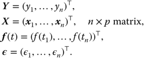
Consider the usual PLM with the form

(7.1)

where is a vector of explanatory variables, is an unknown ‐dimensional parameter vector, the 's are known and nonrandom in some bounded domain , is an unknown smooth function, and 's are i.i.d. random errors with mean 0, variance , which are independent of . PLMs are more flexible than standard linear models since they have both parametric and nonparametric components. They can be a suitable choice when one suspects that the response linearly depends on , but that it is nonlinearly related to .

Surveys regarding the estimation and application of the model (7.1) can be found in the monograph of Hardle et al. (2000). Raheem et al. (2012) considered absolute penalty and shrinkage estimators in PLMs where the vector of coefficients in the linear part can be partitioned as ; is the coefficient vector of the main effects, and is the vector of the nuisance effects. For a more recent study about PLM, we refer to Roozbeh and Arashi (2016b). Since for estimation , we need to estimate the nonparametric component , we estimate it using the kernel smoothing method. Throughout, we do not further discuss the estimation of in PLMs, since the main concern is the estimation of in the ridge context.

To estimate , assume that , satisfy the model (7.1). Since , we have for . Hence, if we know , a natural nonparametric estimator of is given by

(7.2)

where the positive weight function satisfies the three regularity conditions given here:

1. ,
2. ,
3. , where is the indicator function of the set ,
   

These assumptions guarantee the existence of at the optimal convergence rate , in PLMs with probability one. See Müller and Rönz (1999) for more details.

7.2 Partial Linear Model and Estimation

Consider the PLM defined by

(7.3)

where 's are responses, , , are covariates of the unknown vectors, namely, and also , respectively, and are design points, is a real valued function defined on , and are independently and identically distributed (i.i.d.) errors with zero mean and constant variance, .

Our main objective is to estimate when it is suspected that the ‐dimensional sparsity condition may hold. In this situation, we first estimate the parameter using's Speckman's (1988) approach of partial kernel smoothing method, which attains the usual parametric convergence rate without undersmoothing the nonparametric component .

Assume that satisfy the model (7.3). If is the true parameter, then . Also, for , we have

Thus, a natural nonparametric estimator of given is

(7.4)

with the probability weight functions satisfies the three regularity conditions (i)–(iii).

Suppose that we partitioned the design matrix,

and others as

where

To estimate , we minimize

(7.5)

with respect to . This yields the estimator of as

(7.6)

(7.7)

where

respectively.

If is true, then the restricted estimator is

(7.8)

Further, we assume that are i.i.d. random variables and let

Then, the conditional variance of given is , where with . Then, by law of large numbers (LLN),

and the matrix is nonsingular with probability 1. Readers are referred to Shi and Lau (2000), Gao (1995, 1997), and Liang and Härdle (1999), among others. Moreover, for any permutation of as ,

(7.9)

Finally, we use the following assumption:

The functions and satisfy the Lipchitz condition of order 1 on for . Then, we have the following theorem.

As a result of Theorem 7.1, we have the following limiting cases:

1. 
2. 
3. where is the th diagonal element of .

7.3 Ridge Estimators of Regression Parameter

Let the PLM be given as the following form

(7.10)

where

In general, we assume that is an ‐vector of i.i.d. random variables with distribution , where is a symmetric, positive definite known matrix and is an unknown parameter.

Using the model (7.20) and the error distribution of we obtain the maximum likelihood estimator (MLE) or generalized least squares estimator (GLSE) of by minimizing

(7.11)

to get

(7.12)

where , , , and , .

Now, under a restricted modeling paradigm, suppose that satisfies the following linear nonstochastic constraints

(7.13)

where is a nonzero matrix with rank and is a vector of prespecified values. We refer restricted partially linear model (RPLM) to (7.20). For the RPLM, one generally adopts the well‐known GLSE given by

(7.14)

The GLSE is widely used as an unbiased estimator. We refer to Saleh (2006) and Saleh et al. (2014) for more details and applications of restricted parametric or nonparametric models.

Now, in the line of this book, if there exists multicollinearity in , the would be badly apart from the actual coefficient parameter in some directions of ‐dimension space. Hence, instead of minimizing the GLSE objective function as in (7.21), following Roozbeh (2015), one may minimize the objective function where both and are penalty functions

(7.15)

where is a vector of constants.

The resulting estimator is the restricted generalized ridge estimator (GRE), given by

(7.16)

where

(7.17)

is the GRE and is the ridge parameter.

From Saleh (2006), the likelihood ratio criterion for testing the null hypothesis , is given by

(7.18)

where , , is an unbiased estimator of .

Note that follows a noncentral ‐distribution with DF and noncentrality parameter given by

(7.19)

Following Saleh (2006), we define three sorts of estimators using the test statistic . First, we consider the preliminary test generalized ridge estimator (PTGRE) defined by

(7.20)

where is the upper ‐level critical value for the test of and is the indicator function of the set .

This estimator has been considered by Saleh and Kibria (1993). The PTGRE has the disadvantage that it depends on , the level of significance, and also it yields the extreme results, namely, and depending on the outcome of the test.

A nonconvex continuous version of the PTGRE is the Stein‐type generalized ridge estimator (SGRE) defined by

(7.21)

The Stein‐type generalized ridge regression has the disadvantage that it has strange behavior for small values of . Also, the shrinkage factor becomes negative for . Hence, we define the positive‐rule Stein‐type generalized ridge estimator (PRSGRE) given by

(7.22)

Shrinkage estimators have been considered by Arashi and Tabatabaey (2009), Arashi et al. (2010, 2012), Arashi (2012), and extended to monotone functional estimation in multidimensional models just as the additive regression model, semi‐parametric PLM, and generalized linear model by Zhang et al. (2008).

7.4 Biases and Risks of Shrinkage Estimators

In this section, we give exact expressions of the bias and ‐risk functions for the estimators and . Since the properties of unrestricted, restricted, and preliminary test estimators have been widely investigated in the literature, we refer to Sarkar (1992) and Saleh and Kibria (1993) for the properties of unrestricted, restricted, and preliminary test generalized ridge regression estimator.

For analytical comparison between the proposed estimators, we refer to Roozbeh (2015) and continue our study with numerical results.

7.5 Numerical Analysis

To examine the ‐risk performance of the proposed estimators, we adopted the Monte Carlo simulation study of Roozbeh (2015) for illustration.

To achieve different degrees of collinearity, following Kibria (2003) the explanatory variables were generated using the given model for :

where are independent standard normal pseudorandom numbers, and is specified so that the correlation between any two explanatory variables is given by . These variables are then standardized so that and are in correlation forms. Three different sets of correlation corresponding to , and 0.99 are considered. Then observations for the dependent variable are determined by

(7.24)

where , and

which is a mixture of normal densities for and is the normal probability density function (p.d.f.) with mean and variance . The main reason for selecting such a structure for the nonlinear part is to check the efficiency of the nonparametric estimations for wavy function. This function is difficult to estimate and provides a good test case for the nonparametric regression method.

According to Roozbeh (2015), it is assumed , for which the elements of are and . The set of linear restrictions is assumed to have form , where

For the weight function , we use

which is Priestley and Chao's weight with the Gaussian kernel. We also apply the cross‐validation (CV) method to select the optimal bandwidth , which minimizes the following CV function

where obtains by replacing and by

Here, is the predicted value of at with and left out of the estimation of the .

The ratio of largest eigenvalue to smallest eigenvalue of the design matrix in model (7.24) is approximately , and 14 495.28 for , and 0.99, respectively.

In Tables 7.1–7.6, we computed the proposed estimators' risk,

for different values of and .

We found the best values of () by plotting

vs. for each of the proposed estimators (see Figure 7.1).

Figure 7.2 shows the fitted function by kernel smoothing after estimation of the linear part of the model using and , that are, , respectively, for , and 0.99. The minimum of CV approximately obtained was for the model (7.24) with . The diagram of CV vs. is also plotted in Figure 7.3.

From the simulation, we found that at most for superiority of PRSGRE over SGLSE are 0.598, 0.792, and 0.844 for , and 0.99, respectively. It is realized that the ridge parameter is an increasing function of for superiority of PRSGRE over SGRE in ‐risk sense. These values are 0.527, 0.697, and 0.730 for superiority of PRSGRE over PRSGLSE. Finally, the PRSGRE is better than SGRE for all values of and in ‐risk sense.

Coefficients ()	0	0.05	0.10	0.15	0.20	0.25	= 0.299	0.30
	1.007	1.009	1.010	1.012	1.014	1.015	0.994	1.017
	0.900	0.902	0.903	0.905	0.906	0.908	0.995	0.909
	1.986	1.986	1.986	1.986	1.987	1.987	2.004	1.987
	3.024	3.025	3.026	3.027	3.028	3.029	3.004	3.030
	5.073	5.075	5.078	5.081	5.083	5.085	5.002	5.087
	3.999	4.002	4.005	4.008	4.011	4.013	3.996	4.016
	0.274	0.274	0.273	0.273	0.273	0.273	0.273	0.273

Coefficients ()	0	0.05	0.10	0.15	0.20	0.25	= 0.2635	0.30
	1.004	1.002	1.000	0.998	0.996	0.994	0.993	0.992
	1.004	1.002	1.000	0.999	0.997	0.995	0.995	0.994
	2.008	2.007	2.006	2.006	2.005	2.005	2.004	2.004
	3.012	3.010	3.009	3.007	3.006	3.004	3.004	3.003
	5.020	5.016	5.013	5.009	5.006	5.003	5.0021	4.999
	4.016	4.012	4.008	4.004	4.000	3.997	3.996	3.993
	0.242	0.241	0.241	0.241	0.241	0.241	0.241	0.241
	0.027	0.027	0.027	0.028	0.028	0.028	0.028	0.028

Coefficients ()	0	0.10	0.20	0.30	= 0.396	0.40	0.50	0.60
	0.969	0.968	0.966	0.965	0.964	0.964	0.962	0.961
	0.968	0.967	0.966	0.964	0.963	0.963	0.962	0.961
	2.025	2.024	2.024	2.0232	2.022	2.022	2.021	2.020
	3.009	3.008	3.006	3.005	3.003	3.003	3.002	3.001
	5.061	5.058	5.055	5.052 184	5.049	5.048	5.045	5.042
	3.992	3.989	3.985	3.982 498	3.979	3.979	3.975	3.972
	0.540	0.537	0.535	0.534	0.534	0.534	0.534	0.536
	0.090	0.090	0.089	0.089	0.089	0.089	0.088	0.088

Coefficients ()	0	0.10	0.20	0.30	= 0.348	0.40	0.50	0.60
	0.966	0.963	0.956	0.950	0.947	0.943	0.937	0.931
	0.968	0.963	0.957	0.952	0.949	0.946	0.941	0.936
	2.025	2.023	2.021	2.018	2.017	2.016	2.014	2.012
	3.009	3.005	3.000	2.996	2.994	2.991	2.987	2.983
	5.061	5.050	5.039	5.027	5.022	5.016	5.005	4.994
	3.992	3.978	3.965	3.951	3.944	3.937	3.924	3.911
	0.476	0.474	0.472	0.471 787	0.471	0.471	0.472	0.474
	0.0903	0.0905	0.090	0.090	0.090	0.091	0.0912	0.091

Coefficients ()	0	0.10	0.20	0.30	0.40	= 0.422	0.50	0.60
	1.430	1.366	1.308	1.257	1.210	1.200	1.167	1.127
	1.267	1.205	1.150	1.100	1.056	1.046	1.015	0.977
	1.487	1.500	1.510	1.517	1.522	1.523	1.525	1.527
	3.046	3.024	3.001	2.977	2.954	2.949	2.930	2.906
	4.945	4.876	4.811	4.747	4.687	4.674	4.628	4.572
	5.025	4.854	4.700	4.563	4.438	4.412	4.324	4.221
	5.748	5.391	5.179	5.082	5.076	5.085	5.142	5.265
	0.040	0.040	0.041	0.041	0.042	0.042	0.042	0.042

Coefficients ()	0	0.10	0.20	0.30	= 0.365	0.40	0.50	0.60
	1.430	1.340	1.260	1.188	1.144	1.122	1.062	1.007
	1.267	1.179	1.101	1.030	0.987	0.965	0.907	0.854
	1.487	1.496	1.501	1.503	1.503	1.503	1.500	1.496
	3.046	3.007	2.967	2.927	2.901	2.887	2.847	2.808
	4.945	4.834	4.728	4.626	4.562	4.528	4.433	4.342
	5.025	4.786	4.572	4.379	4.264	4.205	4.046	3.901
	5.060	4.752	4.584	4.525	4.534	4.552	4.648	4.798
	0.040	0.041	0.042	0.042	0.043	0.043	0.044	0.045

7.5.1 Example: Housing Prices Data

The housing prices data consist of 92 detached homes in the Ottawa area that were sold during 1987. The variables are defined as follows. The dependent variable is sale price (SP), the independent variables include lot size (lot area; LT), square footage of housing (SFH), average neighborhood income (ANI), distance to highway (DHW), presence of garage (GAR), and fireplace (FP). The full parametric model has the form

(7.25)

Looking at the correlation matrix given in Table 7.7, there exists a potential multicollinearity between variables SFH & FP and DHW & ANI.

We find that the eigenvalues of the matrix are given by , , , , , , and . It is easy to see that the condition number is approximately equal to . So, is morbidity badly.

Variable	SP	LT	SFH	FP	DHW	GAR	ANI
SP	1.00	0.14	0.47	0.33	0.10	0.29	0.34
LT	0.14	1.00	0.15	0.15	0.08	0.16	0.13
SFH	0.47	0.15	1.00	0.46	0.02	0.22	0.27
FP	0.33	0.15	0.46	1.00	0.10	0.14	0.38
DHW	0.10	0.08	0.02	0.10	1.00	0.05	0.10
GAR	0.29	0.16	0.22	0.14	0.05	1.00	0.02
ANI	0.34	0.13	0.27	0.38	0.10	0.02	1.00

An appropriate approach, as a remedy for multicollinearity, is to replace the pure parametric model with a PLM. Akdeniz and Tabakan (2009) proposed a PLM (here termed as semi‐parametric model) for this data by taking the lot area as the nonparametric component.

To realize the type of relation from linearity/nonlinearity viewpoint between dependent variable (SP) and explanatory variables (except for the binary ones), they are plotted in Figure 7.4. According to this figure, we consider the average neighborhood income (ANI) as a nonparametric part. So, the specification of the semi‐parametric model is

(7.26)

To compare the performance of the proposed restricted estimators, following Roozbeh (2015), we consider the parametric restriction , where

The test statistic for testing , given our observations, is

where . Thus, we conclude that the null‐hypothesis is accepted.

Table 7.8 summarizes the results. The “parametric estimates” refer to a model in which ANI enters. In the “semiparametric estimates,” we have used the kernel regression procedure with optimal bandwidth for estimating . For estimating the nonparametric effect, first we estimated the parametric effects and then applied the kernel approach to fit on for , where (Figure 7.5).

	Parametric estimates		Semiparametric estimates
Variable	Coef.	s.e.	Coef.	s.e.
Intercept	62.67	20.69	—	—
LT	0.81	2.65	9.40	2.25
SFH	39.27	11.99	73.45	11.15
FP	6.05	7.68	5.33	8.14
DHW	8.21	6.77	2.22	7.28
GAR	14.47	6.38	12.98	7.20
ANI	0.56	0.28	—	—
	798.0625		149.73
	33 860.06		88 236.41
	0.3329		0.86

The ratio of largest to smallest eigenvalues for the new design matrix in model (7.25) is approximately , and so there exists a potential multicollinearity between the columns of the design matrix. Now, in order to overcome the multicollinearity for better performance of the estimators, we used the proposed estimators for model (7.25).

The SGRRE and PRSGRE for different values of the ridge parameter are given in Tables 7.9 and 7.10, respectively. As it can be seen, is the best estimator for the linear part of the semi‐parametric regression model in the sense of risk.

In Figure 7.6, the and of SGRE (solid line) and PRSGDRE (dash line) vs. ridge parameter are plotted. Finally, we estimated the nonparametric effect () after estimation of the linear part by in Figure 7.7, i.e. we used kernel fit to regress on .

Variable ()	0.0	0.10	0.20	= 0.216	0.30	0.40	0.50	0.60
Intercept	—	—	—	—	—	—	—	—
LT	9.043	9.139	9.235	9.331	9.427	9.250	9.524	9.620
SFH	84.002	84.106	84.195	84.270	84.334	84.208	84.385	84.425
FP	0.460	0.036	0.376	0.777	1.168	0.441	1.549	1.919
DHW	4.086	4.382	4.673	4.960	5.241	4.719	5.519	5.792
GAR	4.924	4.734	4.548	4.367	4.190	4.519	4.017	3.848
ANI	—	—	—	—	—	—	—	—
	257.89	254.09	252.62	252.59	253.35	256.12	260.82	267.31
	2241.81	2241.08	2240.50	2240.42	2240.12	2240.03	2240.02	2240.18

Variable ()	0.0	0.10	= 0.195	0.20	0.30	0.40	0.50	0.60
Intercept	—	—	—	—	—	—	—	—
LT	9.226	9.355	9.476	9.481	9.604	9.725	9.843	9.958
SFH	78.614	77.705	76.860	76.820	75.959	75.120	74.303	73.506
FP	2.953	3.229	3.483	3.495	3.751	3.998	4.237	4.466
DHW	3.136	3.033	2.937	2.933	2.835	2.739	2.645	2.554
GAR	9.042	9.112	9.176	9.179	9.242	9.303	9.362	9.417
ANI	—	—	—	—	—	—	—	—
	234.02	230.68	229.67	230.82	232.68	234.02	239.12	246.00
	2225.762	2233.685	2240.480	2240.838	2248.805	2256.785	2264.771	2272.758

7.6 High‐Dimensional PLM

In this section, we develop the theory proposed in the previous section for the high‐dimensional case in which . For our purpose, we adopt the structure of Arashi and Roozbeh (2016), i.e. we partition the regression parameter as , where the sub‐vector has dimension , and with . Hence, the model (7.20) has the form

(7.27)

where is partitioned according to in such a way that is a sub‐matrix, .

In this section, we consider the estimation of under the sparsity assumption . Hence, we minimize the objective function

(7.28)

where is a function of sample size and is a vector of constants.

The resulting estimator of is the generalized ridge regression estimator (RRE), given by

(7.29)

where and is the generalized restricted estimator of given by

(7.30)

Here, is the bandwidth parameter as a function of sample size , where we estimate by , with is a kernel function of order with bandwidth parameter (see Arashi and Roozbeh 2016).

Note that the generalized (unrestricted) ridge estimators of and , respectively, have the forms

(7.31)

where

In order to derive the forms of shrinkage estimators, we need to find the test statistic for testing the null‐hypothesis . Thus, we make use of the following statistic

(7.32)

where and

(7.33)

To find the asymptotic distribution of , we need to make some regularity conditions. Hence, we suppose the following assumptions hold

1. (A1) (A1) , where is the th row of .
2. (A2) (A2) as ,
3. (A3) (A3) Let
   

   Then, there exists a positive definite matrix such that

   
4. (A4) (A4) .
5. (A5) (A5) , .

Note that by (A2), (A4), and (A5), one can directly conclude that as

(7.34)

The test statistic diverges as , under any fixed alternatives . To overcome this difficulty, in sequel, we consider the local alternatives

where is a fixed vector.

Then, we have the following result about the asymptotic distribution of . The proof is left as an exercise.

Then, in a similar manner to that in Section 5.2, the PTGRE, SGRE, and PRSGRE of are defined respectively as

(7.35)

(7.36)

Under the foregoing regularity conditions (A1)–(A5) and local alternatives , one can derive asymptotic properties of the proposed estimators, which are left as exercise. To end this section, we present in the next section a real data example to illustrate the usefulness of the suggested estimators for high‐dimensional data.

7.6.1 Example: Riboflavin Data

Here, we consider the data set about riboflavin (vitamin ) production in , which can be found in the R package “hdi”. There is a single real‐valued response variable which is the logarithm of the riboflavin production rate. Furthermore, there are explanatory variables measuring the logarithm of the expression level of 4088 genes. There is one rather homogeneous data set from samples that were hybridized repeatedly during a fed batch fermentation process where different engineered strains and strains grown under different fermentation conditions were analyzed. Based on 100‐fold cross‐validation, the LASSO shrinks 4047 parameters to zero and remains significant explanatory variables.

To detect the nonparametric part of the model, for , we calculate

where is obtained by deleting the th column of matrix . Among all 41 remaining genes, “” had minimum value. We also use the added‐variable plots to identify the parametric and nonparametric components of the model. Added‐variable plots enable us to visually assess the effect of each predictor, having adjusted for the effects of the other predictors. By looking at the added‐variable plot (Figure 7.8), we consider “” as a nonparametric part. As it can be seen from this figure, the slope of the least squares line is equal to zero, approximately, and so, the specification of the sparse semi‐parametric regression model is

(7.37)

where and .

For estimating the nonparametric part of the model, , we use

which is Priestley and Chao's weight with the Gaussian kernel.

We also apply the CV method to select the optimal bandwidth and , which minimizes the following CV function

where is obtained by replacing and with , , , , , .

Table 7.11 shows a summary of the results. In this table, the RSS and , respectively, are the residual sum of squares and coefficient of determination of the model, i.e. , and . For estimation of the nonparametric effect, at first we estimated the parametric effects by one of the proposed methods and then the local polynomial approach was applied to fit on , .

Method	GRE	GRRE	SGRRE	PRSGRRE
RSS	16.1187	1.9231	1.3109	1.1509
	0.7282	0.9676	0.9779	0.9806

In this example, as can be seen from Figure 7.8, the nonlinear relation between dependent variable and can be detected, and so the pure parametric model does not fit the data; the semi‐parametric regression model fits more significantly. Further, from Table 7.11, it can be deduced that PRSGRE is quite efficient, in the sense that it has significant value of goodness of fit.

7.7 Summary and Concluding Remarks

In this chapter, apart from the preliminary test and penalty estimators, we mainly concentrated on the Stein‐type shrinkage ridge estimators, for estimating the regression parameters of the partially linear regression models. We developed the problem of ridge estimation for the low/high‐dimensional case. We analyzed the performance of the estimators extensively in Monte Carlo simulations, where the nonparametric component of the model was estimated by the kernel method. The housing prices data used the low‐dimensional part and the riboflavin data used for the high‐dimensional part for practical illustrations, in which the cross‐validation function was applied to obtain the optimal bandwidth parameters.