5
Multiple Linear Regression Models
5.1 Introduction
Traditionally, we use least squares estimators (LSEs) for a linear model which provide minimum variance unbiased estimators. However, data analysts point out two deficiencies of LSEs, namely, the prediction accuracy and the interpretation. To overcome these concerns, Tibshirani (1996) proposed the least absolute shrinkage and selection operator (LASSO). It defines a continuous shrinking operation that can produce coefficients that are exactly zero and is competitive with subset selection and ridge regression estimators (RREs), retaining the good properties of both the estimators. The LASSO simultaneously estimates and selects the coefficients of a given linear model.
However, the preliminary test estimator (PTE) and the Stein‐type estimator only shrink toward the target value and do not select coefficients for appropriate prediction and interpretation.
LASSO is related to the estimators, such as nonnegative garrote by Breiman (1996), smoothly clipped absolute derivation (SCAD) by Fan and Li (2001), elastic net by Zou and Hastie (2005), adaptive LASSO by Zou (2006), hard threshold LASSO by Belloni and Chernozhukov (2013), and many other versions. A general form of an extension of LASSO‐type estimation called the bridge estimation, by Frank and Friedman (1993), is worth pursuing.
This chapter is devoted to the comparative study of the finite sample performance of the primary penalty estimators, namely, LASSO and the RREs. They are compared to the LSE, restricted least squares estimator (RLSE), PTE, SE, and positive‐rule Stein‐type estimator (PRSE) in the context of the multiple linear regression model. The question of comparison between the RRE (first discovery of penalty estimator) and the Stein‐type estimator is well known and is established by Draper and Nostrand (1979), among others. So far, the literature is full of simulated results without any theoretical backups, and definite conclusions are not available whether the design matrix is orthogonal or nonorthogonal. In this chapter, as in the analysis of variance (ANOVA) model, we try to cover some detailed theoretical derivations/comparisons of these estimators in the well‐known multiple linear model.
5.2 Linear Model and the Estimators
Consider the multiple linear model,
where ![]() is the design matrix such that
is the design matrix such that ![]() ,
, ![]() , and
, and ![]() is the response vector. Also,
is the response vector. Also, ![]() is the
is the ![]() ‐vector of errors such that
‐vector of errors such that ![]() ,
, ![]() is the known variance of any
is the known variance of any ![]() (
(![]() ).
).
It is well known that the LSE of ![]() , say,
, say, ![]() , has the distribution
, has the distribution
We designate ![]() as the LSE of
as the LSE of ![]() .
.
In many situations, a sparse model is desired such as high‐dimensional settings. Under the sparsity assumption, we partition the coefficient vector and the design matrix as

where ![]() .
.
Hence, 5.1 may also be written as
where ![]() may stand for the main effects and
may stand for the main effects and ![]() for the interaction which may be insignificant, although one is interested in the estimation and selection of the main effects. Thus, the problem of estimating
for the interaction which may be insignificant, although one is interested in the estimation and selection of the main effects. Thus, the problem of estimating ![]() is reduced to the estimation of
is reduced to the estimation of ![]() when
when ![]() is suspected to be equal to
is suspected to be equal to ![]() . Under this setup, the LSE of
. Under this setup, the LSE of ![]() is
is

and if ![]() , it is
, it is

where ![]() .
.
Note that the marginal distribution of ![]() is
is ![]() and that of
and that of ![]() is
is ![]() . Hence, the weighted
. Hence, the weighted ![]() risk of
risk of ![]() is given by
is given by
Similarly, the weighted ![]() risk of
risk of ![]() is given by
is given by

since the covariance matrix of ![]() is
is ![]() and computation of the risk function of RLSE with
and computation of the risk function of RLSE with ![]() and
and ![]() yields the result 5.7.
yields the result 5.7.
Our focus in this chapter is on the comparative study of the performance properties of three penalty estimators compared to the PTE and the Stein‐type estimator. We refer to Saleh (2006) for the comparative study of PTE and the Stein‐type estimator, when the design matrix is nonorthogonal. We extend the study to include the penalty estimators, which has not been theoretically done yet, except for simulation studies.
5.2.1 Penalty Estimators
Motivated by the idea that only a few regression coefficients contribute to the signal, we consider threshold rules that retain only observed data that exceed a multiple of the noise level. Accordingly, we consider the subset selection rule of Donoho and Johnstone (1994) known as the hard threshold rule, as given by

where ![]() is the
is the ![]() th element of
th element of ![]() ,
, ![]() is an indicator function of the set
is an indicator function of the set ![]() , and marginally
, and marginally

where ![]() .
.
Here, ![]() is the test statistic for testing the null hypothesis
is the test statistic for testing the null hypothesis ![]() vs.
vs. ![]() . The quantity
. The quantity ![]() is called the threshold parameter. The components of
is called the threshold parameter. The components of ![]() are kept as
are kept as ![]() if they are significant and zero, otherwise. It is apparent that each component of
if they are significant and zero, otherwise. It is apparent that each component of ![]() is a PTE of the predictor concerned. The components of
is a PTE of the predictor concerned. The components of ![]() are PTEs and discrete variables and lose some optimality properties. Hence, one may define a continuous version of 5.9 based on marginal distribution of
are PTEs and discrete variables and lose some optimality properties. Hence, one may define a continuous version of 5.9 based on marginal distribution of ![]() (
(![]() ).
).
In accordance with the principle of the PTE approach (see Saleh 2006), we define the Stein‐type estimator as the continuous version of PTE based on the marginal distribution of ![]() ,
, ![]() given by
given by

See Saleh (2006, p. 83) for details.
In order to develop LASSO for our case, we propose the following modified least absolute shrinkage and selection operator (MLASSO) given by
where for ![]() ,
,
The estimator ![]() defines a continuous shrinkage operation that produces a sparse solution.
defines a continuous shrinkage operation that produces a sparse solution.
The formula 5.13 is obtained as follows:
Differentiating ![]() where
where ![]() , we obtain the following equation
, we obtain the following equation
where ![]() and
and ![]() is the
is the ![]() th diagonal element of
th diagonal element of ![]() . Now, the
. Now, the ![]() th marginal component of 5.13 is given by
th marginal component of 5.13 is given by ![]() ,
,
Now, we have two cases:
 , then 5.14 reduces to
(5.16)where
, then 5.14 reduces to
(5.16)where
 . Hence,
(5.17)with, clearly,
. Hence,
(5.17)with, clearly,
 and
and  .
. , then we have
(5.18)
, then we have
(5.18)
Hence,
(5.19)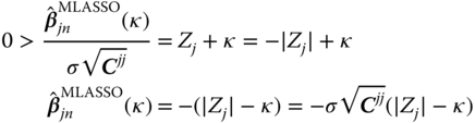
with, clearly,
 and
and  .
.- For
 , we have
  for some
  . Hence, we obtain
  , which implies
  .
.
Combining 5.17, 5.19, and (iii), we obtain 5.13.
Finally, we consider the RREs of ![]() . They are obtained using marginal distributions of
. They are obtained using marginal distributions of ![]() ,
, ![]() , as
, as

to accommodate the sparsity condition; see Tibshirani (1996) on the summary of properties discussed earlier.
In the next section, we define the traditional shrinkage estimators.
5.2.2 Shrinkage Estimators
We recall that the unrestricted estimator of ![]() is given by
is given by ![]() . Using marginal distributions, we have
. Using marginal distributions, we have

The restricted parameter may be denoted by ![]() . Thus, the restricted estimator of
. Thus, the restricted estimator of ![]() is
is ![]() ; see 5.5. Next, we consider the PTE of
; see 5.5. Next, we consider the PTE of ![]() . For this, we first define the test statistic for testing the sparsity hypothesis
. For this, we first define the test statistic for testing the sparsity hypothesis ![]() vs.
vs. ![]() as
as

Indeed, ![]() (chi‐square with
(chi‐square with ![]() degrees of freedom (DF)).
degrees of freedom (DF)).
Thus, define the PTE of ![]() with an upper
with an upper ![]() ‐level of significance as
‐level of significance as

where ![]() stands for the level of significance of the test using
stands for the level of significance of the test using ![]() ,
,
In a similar manner, we define the James–Stein estimator given by

where
The estimator ![]() is not a convex combination of
is not a convex combination of ![]() and
and ![]() and may change the sign opposite to the unrestricted estimator, due to the presence of the term
and may change the sign opposite to the unrestricted estimator, due to the presence of the term ![]() . This is the situation for
. This is the situation for ![]() as well. To avoid this anomaly, we define the PRSE,
as well. To avoid this anomaly, we define the PRSE, ![]() as
as

where
5.3 Bias and Weighted  Risks of Estimators
First, we consider the bias and ![]() risk expressions of the penalty estimators.
risk expressions of the penalty estimators.
5.3.1 Hard Threshold Estimator
Using the results of Donoho and Johnstone (1994), we write the bias and ![]() risk of the hard threshold estimator (HTE), under nonorthogonal design matrices.
risk of the hard threshold estimator (HTE), under nonorthogonal design matrices.
The bias and ![]() risk expressions of
risk expressions of ![]() are given by
are given by
where ![]() is the cumulative distribution function (c.d.f.) of a noncentral chi‐square distribution with 3 DF and noncentrality parameter
is the cumulative distribution function (c.d.f.) of a noncentral chi‐square distribution with 3 DF and noncentrality parameter ![]() (
(![]() ) and the mean square error of
) and the mean square error of ![]() is given by
is given by

Since
Hence,
Thus, we have the revised form of Lemma 1 of Donoho and Johnstone (1994).
The upper bound of ![]() in Lemma 5.1 is independent of
in Lemma 5.1 is independent of ![]() . We may obtain the upper bound of the weighted
. We may obtain the upper bound of the weighted ![]() risk of
risk of ![]() as given here by
as given here by

If we have the sparse solution with ![]() nonzero coefficients,
nonzero coefficients, ![]() ,
, ![]() and
and ![]() zero coefficients
zero coefficients

Thus, the upper bound of a weighted ![]() risk using Lemma 5.1 and 5.26, is given by
risk using Lemma 5.1 and 5.26, is given by
which is independent of ![]() .
.
5.3.2 Modified LASSO
In this section, we provide expressions of bias and mean square errors and weighted ![]() risk. The bias expression for the modified LASSO is given by
risk. The bias expression for the modified LASSO is given by

The ![]() risk of the modified LASSO is given by
risk of the modified LASSO is given by

where

and ![]() .
.
Further, Donoho and Johnstone (1994) gives us the revised Lemma 5.2.
The second upper bound in Lemma 5.2 is free of ![]() . If we have a sparse solution with
. If we have a sparse solution with ![]() nonzero and
nonzero and ![]() zero coefficients such as
zero coefficients such as

then the weighted ![]() ‐risk bound is given by
‐risk bound is given by
which is independent of ![]() .
.
5.3.3 Multivariate Normal Decision Theory and Oracles for Diagonal Linear Projection
Consider the following problem in multivariate normal decision theory. We are given the LSE of ![]() , namely,
, namely, ![]() according to
according to
where ![]() is the marginal variance of
is the marginal variance of ![]() ,
, ![]() , and noise level and
, and noise level and ![]() are the object of interest.
are the object of interest.
We consider a family of diagonal linear projections,
Such estimators keep or kill coordinate. The ideal diagonal coefficients, in this case, are ![]() . These coefficients estimate those
. These coefficients estimate those ![]() 's which are larger than the noise level
's which are larger than the noise level ![]() , yielding the lower bound on the risk as
, yielding the lower bound on the risk as

As a special case of 5.36, we obtain

In general, the risk ![]() cannot be attained for all
cannot be attained for all ![]() by any estimator, linear or nonlinear. However, for the sparse case, if
by any estimator, linear or nonlinear. However, for the sparse case, if ![]() is the number of nonzero coefficients,
is the number of nonzero coefficients, ![]() and
and ![]() is the number of zero coefficients, then 5.38 reduces to the lower bound given by
is the number of zero coefficients, then 5.38 reduces to the lower bound given by
Consequently, the weighted ![]() ‐risk lower bound is given by 5.39 as
‐risk lower bound is given by 5.39 as
As we mentioned earlier, ideal risk cannot be attained, in general, by any estimator, linear or non‐linear. However, in the case of MLASSO and HTE, we revise Theorems 1–4 of Donoho and Johnstone (1994) as follows.
The inequality says that we can mimic the performance of an oracle plus one extra parameter, ![]() , to within a factor of essentially
, to within a factor of essentially ![]() .
.
However, it is natural and more revealing to look for optimal thresholds, ![]() , which yield the smallest possible constant
, which yield the smallest possible constant ![]() in place of
in place of ![]() among soft threshold estimators. We state this in the following theorem.
among soft threshold estimators. We state this in the following theorem.
Finally, we deal with the theorem related to the HTE (subset selection rule).
Here, sufficiently close to ![]() means
means ![]() for some
for some ![]() .
.
5.3.4 Ridge Regression Estimator
We have defined RRE as ![]() in Eq. 5.20. The bias and
in Eq. 5.20. The bias and ![]() risk are then given by
risk are then given by

The weighted ![]() risk is then given by
risk is then given by

The optimum value of ![]() is obtained as
is obtained as ![]() ; so that
; so that

5.3.5 Shrinkage Estimators
We know from Section 5.2.2, the LSE of ![]() is
is ![]() with bias
with bias ![]() and weighted
and weighted ![]() risk given by 5.7, while the restricted estimator of
risk given by 5.7, while the restricted estimator of ![]() is
is ![]() . Then, the bias is equal to
. Then, the bias is equal to ![]() and the weighted
and the weighted ![]() risk is given by 5.8.
risk is given by 5.8.
Next, we consider the PTE of ![]() given by 5.20. Then, the bias and weighted
given by 5.20. Then, the bias and weighted ![]() risk are given by
risk are given by

For the Stein estimator, we have

Similarly, the bias and weighted ![]() risk of the PRSE are given by
risk of the PRSE are given by

5.4 Comparison of Estimators
In this section, we compare various estimators with respect to the LSE, in terms of relative weighted ![]() ‐risk efficiency (RWRE).
‐risk efficiency (RWRE).
5.4.1 Comparison of LSE with RLSE
In this case, the RWRE of RLSE vs. LSE is given by
which is a decreasing function of ![]() . So,
. So,

In order to compute ![]() , we need to find
, we need to find ![]() ,
, ![]() , and
, and ![]() . These are obtained by generating explanatory variables by the following equation based on McDonald and Galarneau (1975),
. These are obtained by generating explanatory variables by the following equation based on McDonald and Galarneau (1975),
where ![]() are independent
are independent ![]() pseudo‐random numbers and
pseudo‐random numbers and ![]() is the correlation between any two explanatory variables. In this study, we take
is the correlation between any two explanatory variables. In this study, we take ![]() , and 0.9 which shows variables are lightly collinear and severely collinear. In our case, we chose
, and 0.9 which shows variables are lightly collinear and severely collinear. In our case, we chose ![]() and various
and various ![]() . The resulting output is then used to compute
. The resulting output is then used to compute ![]() .
.
5.4.2 Comparison of LSE with PTE
Here, the RWRE expression for PTE vs. LSE is given by

where
Then, the PTE outperforms the LSE for

Otherwise, LSE outperforms the PTE in the interval ![]() . We may mention that
. We may mention that ![]() is a decreasing function of
is a decreasing function of ![]() with a maximum at
with a maximum at ![]() , then decreases crossing the 1‐line to a minimum at
, then decreases crossing the 1‐line to a minimum at ![]() with a value
with a value ![]() , and then increases toward the 1‐line.
, and then increases toward the 1‐line.
The ![]() belongs to the interval
belongs to the interval

where ![]() depends on the size of
depends on the size of ![]() and given by
and given by

The quantity ![]() is the value
is the value ![]() at which the RWRE value is minimum.
at which the RWRE value is minimum.
5.4.3 Comparison of LSE with SE and PRSE
Since SE and PRSE need ![]() to express their weighted
to express their weighted ![]() ‐risk expressions, we assume always
‐risk expressions, we assume always ![]() . We have
. We have

It is a decreasing function of ![]() . At
. At ![]() , its value is
, its value is ![]() ; and when
; and when ![]() , its value goes to 1. Hence, for
, its value goes to 1. Hence, for ![]() ,
,

Also,

So that,
5.4.4 Comparison of LSE and RLSE with RRE
First, we consider the weighted ![]() ‐risk difference of LSE and RRE given by
‐risk difference of LSE and RRE given by

Hence, RRE outperforms the LSE uniformly. Similarly, for the RLSE and RRE, the weighted ![]() ‐risk difference is given by
‐risk difference is given by

If ![]() , then 5.59 is negative. Hence, RLSE outperforms RRE at this point. Solving the equation
, then 5.59 is negative. Hence, RLSE outperforms RRE at this point. Solving the equation

For ![]() , we get
, we get

If ![]() , then RLSE performs better than the RRE; and if
, then RLSE performs better than the RRE; and if ![]() , RRE performs better than RLSE. Thus, neither RLSE nor RRE outperforms the other uniformly.
, RRE performs better than RLSE. Thus, neither RLSE nor RRE outperforms the other uniformly.
In addition, the RWRE of RRE vs. LSE equals

which is a decreasing function of ![]() with maximum
with maximum ![]() at
at ![]() and minimum 1 as
and minimum 1 as ![]() . So,
. So,

5.4.5 Comparison of RRE with PTE, SE, and PRSE
5.4.5.1 Comparison Between  and
and 
Here, the weighted ![]() ‐risk difference of
‐risk difference of ![]() and
and ![]() is given by
is given by

Note that the risk of ![]() is an increasing function of
is an increasing function of ![]() crossing the
crossing the ![]() ‐line to a maximum then drops monotonically toward
‐line to a maximum then drops monotonically toward ![]() ‐line as
‐line as ![]() . The value of the risk is
. The value of the risk is ![]() at
at ![]() . On the other hand,
. On the other hand, ![]() is an increasing function of
is an increasing function of ![]() below the
below the ![]() ‐line with a minimum value 0 at
‐line with a minimum value 0 at ![]() and as
and as ![]() ,
, ![]() . Hence, the risk difference in Eq. 5.63 is nonnegative for
. Hence, the risk difference in Eq. 5.63 is nonnegative for ![]() . Thus, the RRE uniformly performs better than PTE.
. Thus, the RRE uniformly performs better than PTE.
5.4.5.2 Comparison Between  and
and 
The weighted ![]() ‐risk difference of
‐risk difference of ![]() and
and ![]() is given by
is given by

Note that the first function is increasing in ![]() with a value 2 at
with a value 2 at ![]() and as
and as ![]() , it tends to
, it tends to ![]() . The second function is also increasing in
. The second function is also increasing in ![]() with a value 0 at
with a value 0 at ![]() and approaches the value
and approaches the value ![]() as
as ![]() . Hence, the risk difference is nonnegative for all
. Hence, the risk difference is nonnegative for all ![]() . Consequently, RRE outperforms SE uniformly.
. Consequently, RRE outperforms SE uniformly.
5.4.5.3 Comparison of  with
with 
The risk of ![]() is
is
where

and ![]() is
is
The weighted ![]() ‐risk difference of PRSE and RRE is given by
‐risk difference of PRSE and RRE is given by

where

Consider the R(![]() ). It is a monotonically increasing function of
). It is a monotonically increasing function of ![]() . At
. At ![]() , its value is
, its value is
and as ![]() , it tends to
, it tends to ![]() . For
. For ![]() , at
, at ![]() , the value is
, the value is ![]() ; and as
; and as ![]() , it tends to
, it tends to ![]() . Hence, the
. Hence, the ![]() risk difference in 5.67 is nonnegative and RRE uniformly outperforms PRSE.
risk difference in 5.67 is nonnegative and RRE uniformly outperforms PRSE.
Note that the risk difference of ![]() and
and ![]() at
at ![]() is
is

because the expected value in Eq. 5.68 is a decreasing function of DF, and ![]() . The risk functions of RRE, PT, SE, and PRSE are plotted in Figures 5.1 and 5.2 for
. The risk functions of RRE, PT, SE, and PRSE are plotted in Figures 5.1 and 5.2 for ![]() and
and ![]() , respectively. These figures are in support of the given comparisons.
, respectively. These figures are in support of the given comparisons.

Figure 5.1 Weighted  risk for the ridge, preliminary test, and Stein‐type and its positive‐rule estimators for
  , and
, and  .
.

Figure 5.2 Weighted  risk for the ridge, preliminary test, and Stein‐type and its positive‐rule estimators for
  , and
, and  .
.
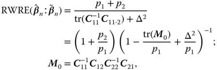
5.4.6 Comparison of MLASSO with LSE and RLSE
First, note that if ![]() coefficients
coefficients ![]() and
and ![]() coefficients are zero in a sparse solution, the lower bound of the weighted
coefficients are zero in a sparse solution, the lower bound of the weighted ![]() risk is given by
risk is given by ![]() . Thereby, we compare all estimators relative to this quantity. Hence, the weighted
. Thereby, we compare all estimators relative to this quantity. Hence, the weighted ![]() ‐risk difference between LSE and MLASSO is given by
‐risk difference between LSE and MLASSO is given by
Hence, if ![]() , the MLASSO performs better than the LSE; while if
, the MLASSO performs better than the LSE; while if ![]() the LSE performs better than the MLASSO. Consequently, neither LSE nor the MLASSO performs better than the other uniformly.
the LSE performs better than the MLASSO. Consequently, neither LSE nor the MLASSO performs better than the other uniformly.
Next, we compare the RLSE and MLASSO. In this case, the weighted ![]() ‐risk difference is given by
‐risk difference is given by
Hence, the RLSE uniformly performs better than the MLASSO.
If ![]() , MLASSO and RLSE are
, MLASSO and RLSE are ![]() ‐risk equivalent. If the LSE estimators are independent, then
‐risk equivalent. If the LSE estimators are independent, then ![]() . Hence, MLASSO satisfies the oracle properties.
. Hence, MLASSO satisfies the oracle properties.
5.4.7 Comparison of MLASSO with PTE, SE, and PRSE
We first consider the PTE vs. MLASSO. In this case, the weighted ![]() ‐risk difference is given by
‐risk difference is given by

Hence, the MLASSO outperforms the PTE when ![]() . When
. When ![]() , the MLASSO outperforms the PTE for
, the MLASSO outperforms the PTE for

Otherwise, PTE outperforms the MLASSO. Hence, neither outperforms the other uniformly.
Next, we consider SE and PRSE vs. the MLASSO. In these two cases, we have weighted ![]() ‐risk differences given by
‐risk differences given by

and from 5.65

where ![]() is given by 5.66. Hence, the MLASSO outperforms the SE as well as the PRSE in the interval
is given by 5.66. Hence, the MLASSO outperforms the SE as well as the PRSE in the interval
Thus, neither SE nor the PRSE outperforms the MLASSO uniformly.
5.4.8 Comparison of MLASSO with RRE
Here, the weighted ![]() ‐risk difference is given by
‐risk difference is given by

Hence, the RRE outperforms the MLASSO uniformly.
5.5 Efficiency in Terms of Unweighted  Risk
Risk
In the previous sections, we have made all comparisons among the estimators in terms of weighted risk functions. In this section, we provide the ![]() ‐risk efficiency of the estimators in terms of the unweighted (weight =
‐risk efficiency of the estimators in terms of the unweighted (weight = ![]() ) risk expressions.
) risk expressions.
The unweighted relative efficiency of the MLASSO:

where ![]() or
or ![]() .
.
The unweighted relative efficiency of the ridge estimator:

The unweighted relative efficiency of PTE:

The unweighted relative efficiency of SE:

where
The unweighted relative efficiency of PRSE:

The unweighted relative efficiency of RRE:

5.6 Summary and Concluding Remarks
In this section, we discuss the contents of Tables 5.1–5.10 presented as confirmatory evidence of the theoretical findings of the estimators.
Table 5.1 Relative weighted ![]() ‐risk efficiency for the estimators for
‐risk efficiency for the estimators for ![]() .
.
| RLSE | PTE | ||||||||||||
| LSE | MLASSO | SE | PRSE | RRE | |||||||||
| 0 | 1 | 4.91 | 5.13 | 5.73 | 5.78 | 4.00 | 2.30 | 2.06 | 1.88 | 2.85 | 3.22 | 4.00 | |
| 0.1 | 1 | 4.79 | 5.00 | 5.57 | 5.62 | 3.92 | 2.26 | 2.03 | 1.85 | 2.82 | 3.15 | 3.92 | |
| 0.5 | 1 | 4.37 | 4.54 | 5.01 | 5.05 | 3.63 | 2.10 | 1.89 | 1.74 | 2.69 | 2.93 | 3.64 | |
| 1 | 1 | 3.94 | 4.08 | 4.45 | 4.48 | 3.33 | 1.93 | 1.76 | 1.62 | 2.55 | 2.71 | 3.36 | |
| 2 | 1 | 3.29 | 3.39 | 3.64 | 3.66 | 2.85 | 1.67 | 1.54 | 1.45 | 2.33 | 2.40 | 2.95 | |
| 3 | 1 | 2.82 | 2.89 | 3.08 | 3.09 | 2.50 | 1.49 | 1.39 | 1.32 | 2.17 | 2.19 | 2.66 | |
| 4.20 | 1 | 2.41 | 2.46 | 2.59 | 2.60 | 2.17 | 1.33 | 1.26 | 1.21 | 2.01 | 2.01 | 2.41 | |
| 4.64 | 1 | 2.29 | 2.34 | 2.45 | 2.46 | 2.07 | 1.29 | 1.23 | 1.18 | 1.97 | 1.96 | 2.34 | |
| 5 | 1 | 2.20 | 2.24 | 2.35 | 2.36 | 2.00 | 1.25 | 1.20 | 1.16 | 1.93 | 1.92 | 2.28 | |
| 5.57 | 1 | 2.07 | 2.11 | 2.20 | 2.21 | 1.89 | 1.21 | 1.16 | 1.13 | 1.88 | 1.86 | 2.20 | |
| 5.64 | 1 | 2.05 | 2.09 | 2.19 | 2.19 | 1.88 | 1.20 | 1.16 | 1.13 | 1.87 | 1.86 | 2.19 | |
| 7 | 1 | 1.80 | 1.83 | 1.90 | 1.91 | 1.66 | 1.12 | 1.09 | 1.07 | 1.77 | 1.76 | 2.04 | |
| 10 | 1 | 1.42 | 1.43 | 1.48 | 1.48 | 1.33 | 1.02 | 1.01 | 1.01 | 1.61 | 1.60 | 1.81 | |
| 15 | 1 | 1.04 | 1.05 | 1.08 | 1.08 | 1.00 | 0.97 | 0.97 | 0.98 | 1.45 | 1.45 | 1.60 | |
| 15.92 | 1 | 1.00 | 1.00 | 1.03 | 1.03 | 0.95 | 0.97 | 0.97 | 0.98 | 1.43 | 1.43 | 1.57 | |
| 16.10 | 1 | 0.99 | 1.00 | 1.02 | 1.02 | 0.94 | 0.97 | 0.97 | 0.98 | 1.43 | 1.42 | 1.56 | |
| 16.51 | 1 | 0.97 | 0.97 | 1.00 | 1.00 | 0.92 | 0.97 | 0.97 | 0.98 | 1.42 | 1.42 | 1.52 | |
| 16.54 | 1 | 0.97 | 0.97 | 0.99 | 1.00 | 0.92 | 0.97 | 0.97 | 0.98 | 1.42 | 1.42 | 1.55 | |
| 20 | 1 | 0.83 | 0.83 | 0.85 | 0.85 | 0.80 | 0.97 | 0.98 | 0.98 | 1.36 | 1.36 | 1.47 | |
| 30 | 1 | 0.58 | 0.59 | 0.59 | 0.59 | 0.57 | 0.99 | 0.99 | 0.99 | 1.25 | 1.25 | 1.33 | |
| 50 | 1 | 0.36 | 0.37 | 0.37 | 0.37 | 0.36 | 0.99 | 0.99 | 1.00 | 1.15 | 1.15 | 1.20 | |
| 100 | 1 | 0.19 | 0.19 | 0.19 | 0.19 | 0.19 | 1.00 | 1.00 | 1.00 | 1.04 | 1.04 | 1.10 | |
Table 5.2 Relative weighted ![]() ‐risk efficiency for the estimators for
‐risk efficiency for the estimators for ![]() .
.
| RLSE | PTE | ||||||||||||
| LSE | MLASSO | SE | PRSE | RRE | |||||||||
| 0 | 1.00 | 8.93 | 9.23 | 9.80 | 9.81 | 5.71 | 2.85 | 2.49 | 2.22 | 4.44 | 4.91 | 5.71 | |
| 0.1 | 1.00 | 8.74 | 9.02 | 9.56 | 9.58 | 5.63 | 2.81 | 2.46 | 2.20 | 4.39 | 4.84 | 5.63 | |
| 0.5 | 1.00 | 8.03 | 8.27 | 8.72 | 8.74 | 5.33 | 2.66 | 2.33 | 2.09 | 4.22 | 4.57 | 5.33 | |
| 1 | 1.00 | 7.30 | 7.49 | 7.86 | 7.88 | 5.00 | 2.49 | 2.20 | 1.98 | 4.03 | 4.28 | 5.01 | |
| 2 | 1.00 | 6.17 | 6.31 | 6.57 | 6.58 | 4.44 | 2.20 | 1.97 | 1.79 | 3.71 | 3.83 | 4.50 | |
| 3 | 1.00 | 5.34 | 5.45 | 5.64 | 5.65 | 4.00 | 1.98 | 1.79 | 1.65 | 3.44 | 3.50 | 4.10 | |
| 5 | 1.00 | 4.21 | 4.28 | 4.40 | 4.40 | 3.33 | 1.67 | 1.53 | 1.43 | 3.05 | 3.05 | 3.52 | |
| 7 | 1.00 | 3.48 | 3.52 | 3.60 | 3.61 | 2.85 | 1.45 | 1.36 | 1.29 | 2.76 | 2.74 | 3.13 | |
| 10 | 1.00 | 2.76 | 2.78 | 2.83 | 2.84 | 2.35 | 1.26 | 1.20 | 1.16 | 2.45 | 2.43 | 2.72 | |
| 10.46 | 1.00 | 2.67 | 2.70 | 2.74 | 2.75 | 2.29 | 1.23 | 1.18 | 1.14 | 2.41 | 2.39 | 2.67 | |
| 10.79 | 1.00 | 2.61 | 2.64 | 2.68 | 2.68 | 2.24 | 1.22 | 1.17 | 1.13 | 2.39 | 2.37 | 2.64 | |
| 11.36 | 1.00 | 2.52 | 2.54 | 2.58 | 2.58 | 2.17 | 1.19 | 1.15 | 1.12 | 2.34 | 2.33 | 2.58 | |
| 11.38 | 1.00 | 2.52 | 2.54 | 2.58 | 2.58 | 2.17 | 1.19 | 1.15 | 1.12 | 2.34 | 2.32 | 2.58 | |
| 15 | 1.00 | 2.05 | 2.06 | 2.09 | 2.09 | 1.81 | 1.09 | 1.06 | 1.05 | 2.12 | 2.11 | 2.31 | |
| 20 | 1.00 | 1.63 | 1.64 | 1.66 | 1.66 | 1.48 | 1.02 | 1.01 | 1.01 | 1.91 | 1.91 | 2.05 | |
| 30 | 1.00 | 1.16 | 1.16 | 1.17 | 1.17 | 1.08 | 0.99 | 0.99 | 0.99 | 1.66 | 1.66 | 1.76 | |
| 33 | 1.00 | 1.06 | 1.07 | 1.07 | 1.07 | 1.00 | 0.99 | 0.99 | 0.99 | 1.61 | 1.61 | 1.70 | |
| 35.52 | 1.00 | 1.00 | 1.00 | 1.01 | 1.01 | 0.94 | 0.99 | 0.99 | 0.99 | 1.58 | 1.57 | 1.65 | |
| 35.66 | 1.00 | 0.99 | 1.00 | 1.00 | 1.00 | 0.93 | 0.99 | 0.99 | 0.99 | 1.57 | 1.57 | 1.65 | |
| 35.91 | 1.00 | 0.99 | 0.99 | 1.00 | 1.02 | 0.93 | 0.99 | 0.99 | 0.99 | 1.57 | 1.57 | 1.65 | |
| 35.92 | 1.00 | 0.99 | 0.99 | 0.99 | 1.00 | 0.93 | 0.99 | 0.99 | 0.99 | 1.57 | 1.57 | 1.65 | |
| 50 | 1.00 | 0.73 | 0.73 | 0.73 | 0.73 | 0.70 | 0.99 | 0.99 | 0.99 | 1.43 | 1.43 | 1.48 | |
| 100 | 1.00 | 0.38 | 0.38 | 0.38 | 0.38 | 0.37 | 1.00 | 1.00 | 1.00 | 1.12 | 1.12 | 1.25 | |
Table 5.3 Relative weighted ![]() ‐risk efficiency of the estimators for
‐risk efficiency of the estimators for ![]() and different
and different ![]() values for varying
values for varying ![]() .
.
| Estimators | ||||||||
| LSE | 1.00 | 1.00 | 1.00 | 1.00 | 1.00 | 1.00 | 1.00 | 1.00 |
| RLSE ( |
5.68 | 3.71 | 2.15 | 1.49 | 3.62 | 2.70 | 1.77 | 1.30 |
| RLSE ( |
6.11 | 3.93 | 2.23 | 1.52 | 3.79 | 2.82 | 1.82 | 1.32 |
| RLSE ( |
9.45 | 5.05 | 2.54 | 1.67 | 4.85 | 3.35 | 2.03 | 1.43 |
| RLSE ( |
10.09 | 5.18 | 2.58 | 1.68 | 5.02 | 3.41 | 2.05 | 1.44 |
| MLASSO | 5.00 | 3.33 | 2.00 | 1.42 | 3.33 | 2.50 | 1.66 | 1.25 |
| PTE ( |
2.34 | 1.97 | 1.51 | 1.22 | 1.75 | 1.55 | 1.27 | 1.08 |
| PTE ( |
2.06 | 1.79 | 1.42 | 1.19 | 1.60 | 1.44 | 1.22 | 1.06 |
| PTE ( |
1.86 | 1.65 | 1.36 | 1.16 | 1.49 | 1.37 | 1.18 | 1.05 |
| SE | 2.50 | 2.00 | 1.42 | 1.11 | 2.13 | 1.77 | 1.32 | 1.07 |
| PRSE | 3.03 | 2.31 | 1.56 | 1.16 | 2.31 | 1.88 | 1.38 | 1.10 |
| RRE | 5.00 | 3.33 | 2.00 | 1.42 | 3.46 | 2.58 | 1.71 | 1.29 |
| LSE | 1.00 | 1.00 | 1.00 | 1.00 | 1.00 | 1.00 | 1.00 | 1.00 |
| RLSE ( |
1.47 | 1.30 | 1.03 | 0.85 | 0.85 | 0.78 | 0.68 | 0.59 |
| RLSE ( |
1.50 | 1.32 | 1.05 | 0.86 | 0.85 | 0.79 | 0.69 | 0.60 |
| RLSE ( |
1.65 | 1.43 | 1.12 | 0.91 | 0.90 | 0.83 | 0.71 | 0.62 |
| RLSE ( |
1.66 | 1.44 | 1.12 | 0.91 | 0.90 | 0.83 | 0.72 | 0.62 |
| MLASSO | 1.42 | 1.25 | 1.00 | 0.83 | 0.83 | 0.76 | 0.66 | 0.58 |
| PTE ( |
1.05 | 1.00 | 0.94 | 0.91 | 0.92 | 0.91 | 0.91 | 0.93 |
| PTE ( |
1.03 | 1.00 | 0.95 | 0.93 | 0.93 | 0.93 | 0.93 | 0.95 |
| PTE ( |
1.02 | 0.99 | 0.95 | 0.94 | 0.94 | 0.94 | 0.95 | 0.96 |
| SE | 1.55 | 1.38 | 1.15 | 1.02 | 1.32 | 1.22 | 1.08 | 1.01 |
| PRSE | 1.53 | 1.37 | 1.15 | 1.02 | 1.31 | 1.21 | 1.08 | 1.01 |
| RRE | 1.96 | 1.69 | 1.33 | 1.12 | 1.55 | 1.40 | 1.20 | 1.07 |
| LSE | 1.00 | 1.00 | 1.00 | 1.00 | 1.00 | 1.00 | 1.00 | 1.00 |
| RLSE ( |
0.45 | 0.44 | 0.40 | 0.37 | 0.16 | 0.15 | 0.15 | 0.14 |
| RLSE ( |
0.46 | 0.44 | 0.40 | 0.37 | 0.16 | 0.15 | 0.15 | 0.15 |
| RLSE ( |
0.47 | 0.45 | 0.41 | 0.38 | 0.16 | 0.16 | 0.15 | 0.15 |
| RLSE ( |
0.47 | 0.45 | 0.41 | 0.38 | 0.16 | 0.16 | 0.15 | 0.15 |
| MLASSO | 0.45 | 0.43 | 0.40 | 0.37 | 0.16 | 0.15 | 0.15 | 0.14 |
| PTE ( |
0.96 | 0.97 | 0.98 | 0.99 | 1.00 | 1.00 | 1.00 | 1.00 |
| PTE ( |
0.97 | 0.98 | 0.98 | 0.99 | 1.00 | 1.00 | 1.00 | 1.00 |
| PTE ( |
0.98 | 0.98 | 0.99 | 0.99 | 1.00 | 1.00 | 1.00 | 1.00 |
| SE | 1.17 | 1.12 | 1.04 | 1.00 | 1.05 | 1.04 | 1.01 | 1.00 |
| PRSE | 1.17 | 1.11 | 1.04 | 1.00 | 1.05 | 1.04 | 1.01 | 1.00 |
| RRE | 1.29 | 1.22 | 1.11 | 1.04 | 1.10 | 1.07 | 1.04 | 1.01 |
Table 5.4 Relative weighted ![]() ‐risk efficiency of the estimators for
‐risk efficiency of the estimators for ![]() and different
and different ![]() values for varying
values for varying ![]()
| Estimators | ||||||||
| LSE | 1.00 | 1.00 | 1.00 | 1.00 | 1.00 | 1.00 | 1.00 | 1.00 |
| RLSE ( |
12.98 | 8.50 | 4.92 | 3.39 | 7.86 | 5.96 | 3.95 | 2.90 |
| RLSE ( |
14.12 | 9.05 | 5.14 | 3.54 | 8.27 | 6.22 | 4.09 | 2.98 |
| RLSE ( |
21.56 | 11.44 | 5.74 | 3.76 | 10.47 | 7.36 | 4.59 | 3.25 |
| RLSE ( |
22.85 | 11.73 | 5.79 | 3.78 | 10.65 | 7.39 | 4.49 | 3.18 |
| MLASSO | 10.00 | 6.66 | 4.00 | 2.85 | 6.66 | 5.00 | 3.33 | 2.50 |
| PTE ( |
3.20 | 2.83 | 2.30 | 1.94 | 2.49 | 2.27 | 1.93 | 1.67 |
| PTE ( |
2.69 | 2.44 | 2.06 | 1.79 | 2.17 | 2.01 | 1.76 | 1.56 |
| PTE ( |
2.34 | 2.16 | 1.88 | 1.66 | 1.94 | 1.82 | 1.62 | 1.47 |
| SE | 5.00 | 4.00 | 2.85 | 2.22 | 4.12 | 3.42 | 2.55 | 2.04 |
| PRSE | 6.27 | 4.77 | 3.22 | 2.43 | 4.57 | 3.72 | 2.71 | 2.13 |
| RRE | 10.00 | 6.66 | 4.00 | 2.85 | 6.78 | 5.07 | 3.36 | 2.52 |
| LSE | 1.00 | 1.00 | 1.00 | 1.00 | 1.00 | 1.00 | 1.00 | 1.00 |
| RLSE ( |
3.05 | 2.71 | 2.20 | 1.83 | 1.73 | 1.61 | 1.42 | 1.25 |
| RLSE ( |
3.11 | 2.77 | 2.25 | 1.87 | 1.75 | 1.63 | 1.44 | 1.27 |
| RLSE ( |
3.37 | 2.96 | 2.35 | 1.93 | 1.82 | 1.70 | 1.48 | 1.30 |
| RLSE ( |
3.40 | 2.98 | 2.36 | 1.94 | 1.83 | 1.70 | 1.48 | 1.30 |
| MLASSO | 2.85 | 2.50 | 2.00 | 1.66 | 1.66 | 1.53 | 1.33 | 1.17 |
| PTE ( |
1.42 | 1.36 | 1.25 | 1.17 | 1.07 | 1.05 | 1.02 | 0.99 |
| PTE ( |
1.33 | 1.28 | 1.20 | 1.13 | 1.05 | 1.04 | 1.01 | 0.99 |
| PTE ( |
1.26 | 1.23 | 1.16 | 1.11 | 1.04 | 1.03 | 1.01 | 0.99 |
| SE | 2.65 | 2.35 | 1.93 | 1.64 | 2.02 | 1.86 | 1.61 | 1.43 |
| PRSE | 2.63 | 2.34 | 1.92 | 1.63 | 2.00 | 1.85 | 1.60 | 1.42 |
| RRE | 3.38 | 2.91 | 2.28 | 1.88 | 2.37 | 2.15 | 1.81 | 1.58 |
| LSE | 1.00 | 1.00 | 1.00 | 1.00 | 1.00 | 1.00 | 1.00 | 1.00 |
| RLSE ( |
0.92 | 0.87 | 0.83 | 0.77 | 0.32 | 0.32 | 0.31 | 0.30 |
| RLSE ( |
0.93 | 0.90 | 0.83 | 0.77 | 0.32 | 0.32 | 0.31 | 0.30 |
| RLSE ( |
0.95 | 0.91 | 0.85 | 0.79 | 0.32 | 0.32 | 0.31 | 0.30 |
| RLSE ( |
0.95 | 0.92 | 0.85 | 0.79 | 0.32 | 0.32 | 0.31 | 0.30 |
| MLASSO | 0.90 | 0.86 | 0.80 | 0.74 | 0.32 | 0.31 | 0.30 | 0.29 |
| PTE ( |
0.97 | 0.97 | 0.97 | 0.97 | 1.00 | 1.00 | 1.00 | 1.00 |
| PTE ( |
0.98 | 0.98 | 0.98 | 0.98 | 1.00 | 1.00 | 1.00 | 1.00 |
| PTE ( |
0.98 | 0.98 | 0.98 | 0.98 | 1.00 | 1.00 | 1.00 | 1.00 |
| SE | 1.57 | 1.49 | 1.36 | 1.25 | 1.20 | 1.18 | 1.13 | 1.09 |
| PRSE | 1.57 | 1.49 | 1.36 | 1.25 | 1.20 | 1.18 | 1.13 | 1.09 |
| RRE | 1.74 | 1.64 | 1.47 | 1.34 | 1.26 | 1.23 | 1.17 | 1.13 |
Table 5.5 Relative weighted ![]() ‐risk efficiency of the estimators for
‐risk efficiency of the estimators for ![]() and different
and different ![]() values for varying
values for varying ![]() .
.
| Estimators | ||||||||
| LSE | 1.00 | 1.00 | 1.00 | 1.00 | 1.00 | 1.00 | 1.00 | 1.00 |
| RLSE ( |
34.97 | 22.73 | 13.02 | 8.95 | 18.62 | 14.47 | 9.82 | 7.31 |
| RLSE ( |
38.17 | 24.29 | 13.64 | 9.24 | 19.49 | 15.09 | 10.16 | 7.50 |
| RLSE ( |
57.97 | 30.39 | 15.05 | 9.80 | 23.60 | 17.24 | 10.93 | 7.87 |
| RLSE ( |
61.39 | 30.94 | 15.20 | 9.83 | 24.15 | 17.42 | 11.01 | 7.89 |
| MLASSO | 20.00 | 13.33 | 8.00 | 5.71 | 13.33 | 10.00 | 6.66 | 5.00 |
| PTE ( |
4.04 | 3.73 | 3.23 | 2.85 | 3.32 | 3.11 | 2.76 | 2.49 |
| PTE ( |
3.28 | 3.08 | 2.76 | 2.49 | 2.77 | 2.63 | 2.39 | 2.20 |
| PTE ( |
2.77 | 2.64 | 2.41 | 2.22 | 2.39 | 2.30 | 2.13 | 1.98 |
| SE | 10.00 | 8.00 | 5.71 | 4.44 | 8.12 | 6.75 | 5.05 | 4.03 |
| PRSE | 12.80 | 9.69 | 6.52 | 4.91 | 9.24 | 7.50 | 5.45 | 4.28 |
| RRE | 20.00 | 13.33 | 8.00 | 5.71 | 13.44 | 10.06 | 6.69 | 5.01 |
| LSE | 1.00 | 1.00 | 1.00 | 1.00 | 1.00 | 1.00 | 1.00 | 1.00 |
| RLSE ( |
6.50 | 5.91 | 4.95 | 4.22 | 3.58 | 3.39 | 3.05 | 2.76 |
| RLSE ( |
6.58 | 6.00 | 5.04 | 4.30 | 3.61 | 3.43 | 3.09 | 2.79 |
| RLSE ( |
7.02 | 6.32 | 5.22 | 4.40 | 3.73 | 3.53 | 3.15 | 2.83 |
| RLSE ( |
7.06 | 6.35 | 5.23 | 4.40 | 3.75 | 3.54 | 3.16 | 2.84 |
| MLASSO | 5.71 | 5.00 | 4.00 | 3.33 | 3.33 | 3.07 | 2.66 | 2.35 |
| PTE ( |
1.96 | 1.89 | 1.77 | 1.67 | 1.37 | 1.35 | 1.30 | 1.26 |
| PTE ( |
1.75 | 1.70 | 1.61 | 1.53 | 1.29 | 1.27 | 1.23 | 1.20 |
| PTE ( |
1.60 | 1.56 | 1.49 | 1.43 | 1.23 | 1.21 | 1.18 | 1.16 |
| SE | 4.87 | 4.35 | 3.58 | 3.05 | 3.45 | 3.19 | 2.77 | 2.45 |
| PRSE | 4.88 | 4.35 | 3.58 | 3.05 | 3.41 | 3.16 | 2.75 | 2.43 |
| RRE | 6.23 | 5.40 | 4.26 | 3.52 | 4.03 | 3.67 | 3.13 | 2.72 |
| LSE | 1.00 | 1.00 | 1.00 | 1.00 | 1.00 | 1.00 | 1.00 | 1.00 |
| RLSE ( |
1.89 | 1.83 | 1.73 | 1.63 | 0.65 | 0.64 | 0.63 | 0.62 |
| RLSE ( |
1.93 | 1.87 | 1.76 | 1.66 | 0.65 | 0.64 | 0.63 | 0.62 |
| RLSE ( |
1.92 | 1.86 | 1.76 | 1.66 | 0.65 | 0.65 | 0.63 | 0.62 |
| RLSE ( |
1.93 | 1.87 | 1.76 | 1.66 | 0.65 | 0.65 | 0.63 | 0.62 |
| MLASSO | 1.81 | 1.73 | 1.60 | 1.48 | 0.64 | 0.63 | 0.61 | 0.59 |
| PTE ( |
1.05 | 1.04 | 1.03 | 1.02 | 0.99 | 0.99 | 0.99 | 0.99 |
| PTE ( |
1.03 | 1.03 | 1.02 | 1.01 | 0.99 | 0.99 | 0.99 | 0.99 |
| PTE ( |
1.02 | 1.02 | 1.01 | 1.01 | 0.99 | 0.99 | 1.00 | 1.00 |
| SE | 2.41 | 2.29 | 2.08 | 1.91 | 1.51 | 1.48 | 1.42 | 1.36 |
| PRSE | 2.40 | 2.28 | 2.08 | 1.91 | 1.51 | 1.48 | 1.42 | 1.36 |
| RRE | 2.64 | 2.50 | 2.25 | 2.05 | 1.58 | 1.54 | 1.47 | 1.41 |
Table 5.6 Relative weighted ![]() ‐risk efficiency of the estimators for
‐risk efficiency of the estimators for ![]() and different
and different ![]() values for varying
values for varying ![]() .
.
| Estimators | ||||||||
| LSE | 1.00 | 1.00 | 1.00 | 1.00 | 1.00 | 1.00 | 1.00 | 1.00 |
| RLSE ( |
78.67 | 50.45 | 28.36 | 19.22 | 33.91 | 27.33 | 19.24 | 14.553 |
| RLSE ( |
85.74 | 53.89 | 29.66 | 19.83 | 35.15 | 28.31 | 19.82 | 14.89 |
| RLSE ( |
130.12 | 67.07 | 32.66 | 20.97 | 40.85 | 31.57 | 21.12 | 15.52 |
| RLSE ( |
138.26 | 68.81 | 33.13 | 21.00 | 41.62 | 31.95 | 21.31 | 15.58 |
| MLASSO | 30.00 | 20.00 | 12.00 | 8.57 | 20.00 | 15.00 | 10.00 | 7.50 |
| PTE ( |
4.49 | 4.22 | 3.78 | 3.42 | 3.80 | 3.61 | 3.29 | 3.02 |
| PTE ( |
3.58 | 3.42 | 3.14 | 2.90 | 3.10 | 2.98 | 2.77 | 2.59 |
| PTE ( |
2.99 | 2.88 | 2.70 | 2.53 | 2.64 | 2.56 | 2.41 | 2.28 |
| SE | 15.00 | 12.00 | 8.57 | 6.66 | 12.12 | 10.08 | 7.55 | 6.03 |
| PRSE | 19.35 | 14.63 | 9.83 | 7.40 | 13.98 | 11.33 | 8.22 | 6.45 |
| RRE | 30.00 | 20.00 | 12.00 | 8.57 | 20.11 | 15.06 | 10.02 | 7.51 |
| LSE | 1.00 | 1.00 | 1.00 | 1.00 | 1.00 | 1.00 | 1.00 | 1.00 |
| RLSE ( |
10.39 | 9.67 | 8.42 | 7.38 | 5.56 | 5.35 | 4.94 | 4.57 |
| RLSE ( |
10.50 | 9.79 | 8.53 | 7.47 | 5.60 | 5.39 | 4.98 | 4.60 |
| RLSE ( |
10.96 | 10.16 | 8.76 | 7.62 | 5.72 | 5.50 | 5.06 | 4.66 |
| RLSE ( |
11.02 | 10.20 | 8.79 | 7.63 | 5.74 | 5.58 | 5.07 | 4.66 |
| MLASSO | 8.57 | 7.50 | 6.00 | 5.00 | 5.00 | 4.61 | 4.00 | 3.52 |
| PTE ( |
2.35 | 2.28 | 2.16 | 2.04 | 1.63 | 1.60 | 1.54 | 1.50 |
| PTE ( |
2.04 | 1.99 | 1.90 | 1.82 | 1.48 | 1.46 | 1.42 | 1.39 |
| PTE ( |
1.82 | 1.79 | 1.72 | 1.67 | 1.38 | 1.37 | 1.34 | 1.31 |
| SE | 7.09 | 6.35 | 5.25 | 4.47 | 4.88 | 4.53 | 3.94 | 3.50 |
| PRSE | 7.16 | 6.40 | 5.28 | 4.49 | 4.83 | 4.48 | 3.91 | 3.47 |
| RRE | 9.08 | 7.89 | 6.26 | 5.18 | 5.69 | 5.21 | 4.45 | 3.89 |
| LSE | 1.00 | 1.00 | 1.00 | 1.00 | 1.00 | 1.00 | 1.00 | 1.00 |
| RLSE ( |
2.88 | 2.83 | 2.71 | 2.59 | 0.98 | 0.98 | 0.96 | 0.95 |
| RLSE ( |
2.89 | 2.84 | 2.72 | 2.60 | 0.98 | 0.98 | 0.96 | 0.95 |
| RLSE ( |
2.93 | 2.87 | 2.74 | 2.62 | 0.99 | 0.98 | 0.97 | 0.95 |
| RLSE ( |
2.93 | 2.87 | 2.74 | 2.62 | 0.99 | 0.98 | 0.97 | 0.95 |
| MLASSO | 2.72 | 2.60 | 2.40 | 2.22 | 0.96 | 0.95 | 0.92 | 0.89 |
| PTE ( |
1.15 | 1.14 | 1.12 | 1.11 | 0.99 | 0.99 | 0.99 | 0.99 |
| PTE ( |
1.11 | 1.10 | 1.09 | 1.08 | 0.99 | 0.99 | 0.99 | 0.99 |
| PTE ( |
1.08 | 1.07 | 1.07 | 1.06 | 0.99 | 0.99 | 0.99 | 0.99 |
| SE | 3.25 | 3.09 | 2.82 | 2.60 | 1.83 | 1.79 | 1.77 | 1.65 |
| PRSE | 3.23 | 3.08 | 2.81 | 2.55 | 1.83 | 1.79 | 1.71 | 1.65 |
| RRE | 3.55 | 3.36 | 3.05 | 2.78 | 1.90 | 1.86 | 1.78 | 1.70 |
Table 5.7 Relative weighted ![]() ‐risk efficiency values of estimators for
‐risk efficiency values of estimators for ![]() and different values of
and different values of ![]() and
and ![]() .
.
| RLSE | PTE | |||||||||
| LSE | 0.8 | 0.9 | MLASSO | 0.25 | SE | PRSE | RRE | |||
| 5 | 1.00 | 2.00 | 2.02 | 1.71 | 1.56 | 1.39 | 1.28 | 1.33 | 1.42 | 1.71 |
| 15 | 1.00 | 4.14 | 4.15 | 3.14 | 2.62 | 2.06 | 1.74 | 2.44 | 2.68 | 3.14 |
| 25 | 1.00 | 6.81 | 6.84 | 4.57 | 3.52 | 2.55 | 2.04 | 3.55 | 3.92 | 4.57 |
| 35 | 1.00 | 10.28 | 10.32 | 6.00 | 4.32 | 2.92 | 2.26 | 4.66 | 5.16 | 6.00 |
| 55 | 1.00 | 21.72 | 21.75 | 8.85 | 5.66 | 3.47 | 2.56 | 6.88 | 7.65 | 8.85 |
| 5 | 1.00 | 1.85 | 1.86 | 1.60 | 1.43 | 1.29 | 1.20 | 1.29 | 1.35 | 1.60 |
| 15 | 1.00 | 3.78 | 3.79 | 2.93 | 2.40 | 1.90 | 1.63 | 2.33 | 2.49 | 2.93 |
| 25 | 1.00 | 6.15 | 6.18 | 4.26 | 3.24 | 2.36 | 1.92 | 3.38 | 3.64 | 4.27 |
| 35 | 1.00 | 9.16 | 9.19 | 5.60 | 3.98 | 2.72 | 2.13 | 4.43 | 4.80 | 5.60 |
| 55 | 1.00 | 18.48 | 18.49 | 8.26 | 5.24 | 3.25 | 2.42 | 6.54 | 7.11 | 8.27 |
| 5 | 1.00 | 1.71 | 1.73 | 1.50 | 1.33 | 1.21 | 1.14 | 1.26 | 1.29 | 1.53 |
| 15 | 1.00 | 3.48 | 3.49 | 2.75 | 2.22 | 1.78 | 1.54 | 2.24 | 2.34 | 2.77 |
| 25 | 1.00 | 5.61 | 5.63 | 4.00 | 3.00 | 2.21 | 1.81 | 3.23 | 3.42 | 4.01 |
| 35 | 1.00 | 8.26 | 8.28 | 5.25 | 3.69 | 2.55 | 2.02 | 4.23 | 4.50 | 5.26 |
| 55 | 1.00 | 16.07 | 16.09 | 7.75 | 4.88 | 3.06 | 2.31 | 6.23 | 6.67 | 7.76 |
| 5 | 1.00 | 1.09 | 1.09 | 1.00 | 0.94 | 0.95 | 0.96 | 1.12 | 1.12 | 1.26 |
| 15 | 1.00 | 2.13 | 2.13 | 1.83 | 1.41 | 1.23 | 1.14 | 1.78 | 1.77 | 2.04 |
| 25 | 1.00 | 3.29 | 3.30 | 2.66 | 1.86 | 1.48 | 1.31 | 2.48 | 2.47 | 2.86 |
| 35 | 1.00 | 4.62 | 4.63 | 3.50 | 2.28 | 1.71 | 1.46 | 3.19 | 3.19 | 3.69 |
| 55 | 1.00 | 7.88 | 7.89 | 5.16 | 3.04 | 2.08 | 1.69 | 4.61 | 4.64 | 5.35 |
Table 5.8 Relative weighted ![]() ‐risk efficiency values of estimators for
‐risk efficiency values of estimators for ![]() and different values of
and different values of ![]() and
and ![]() .
.
| RLSE | PTE | |||||||||
| LSE | 0.8 | 0.9 | MLASSO | 0.25 | SE | PRSE | RRE | |||
| 3 | 1.00 | 1.67 | 1.68 | 1.42 | 1.33 | 1.22 | 1.16 | 1.11 | 1.16 | 1.42 |
| 13 | 1.00 | 3.76 | 3.78 | 2.85 | 2.41 | 1.94 | 1.66 | 2.22 | 2.43 | 2.85 |
| 23 | 1.00 | 6.38 | 6.42 | 4.28 | 3.34 | 2.46 | 1.99 | 3.33 | 3.67 | 4.28 |
| 33 | 1.00 | 9.79 | 9.84 | 5.71 | 4.16 | 2.85 | 2.22 | 4.44 | 4.91 | 5.71 |
| 53 | 1.00 | 21.01 | 21.05 | 8.57 | 5.54 | 3.42 | 2.53 | 6.66 | 7.40 | 8.57 |
| 3 | 1.00 | 1.54 | 1.55 | 1.33 | 1.23 | 1.14 | 1.10 | 1.09 | 1.12 | 1.34 |
| 13 | 1.00 | 3.43 | 3.45 | 2.66 | 2.22 | 1.80 | 1.56 | 2.12 | 2.26 | 2.67 |
| 23 | 1.00 | 5.77 | 5.79 | 4.00 | 3.08 | 2.28 | 1.87 | 3.17 | 3.41 | 4.00 |
| 33 | 1.00 | 8.72 | 8.76 | 5.33 | 3.84 | 2.66 | 2.09 | 4.22 | 4.57 | 5.33 |
| 53 | 1.00 | 17.87 | 17.90 | 8.00 | 5.13 | 3.21 | 2.40 | 6.33 | 6.88 | 8.00 |
| 3 | 1.00 | 1.43 | 1.44 | 1.25 | 1.14 | 1.08 | 1.05 | 1.07 | 1.10 | 1.29 |
| 13 | 1.00 | 3.16 | 3.18 | 2.50 | 2.05 | 1.67 | 1.47 | 2.04 | 2.13 | 2.52 |
| 23 | 1.00 | 5.26 | 5.28 | 3.75 | 2.85 | 2.13 | 1.76 | 3.03 | 3.20 | 3.76 |
| 33 | 1.00 | 7.86 | 7.90 | 5.00 | 3.56 | 2.49 | 1.98 | 4.03 | 4.28 | 5.01 |
| 53 | 1.00 | 15.55 | 15.57 | 7.50 | 4.77 | 3.02 | 2.28 | 6.03 | 6.45 | 7.51 |
| 3 | 1.00 | 0.91 | 0.91 | 0.83 | 0.86 | 0.91 | 0.94 | 1.02 | 1.02 | 1.12 |
| 13 | 1.00 | 1.93 | 1.94 | 1.66 | 1.31 | 1.17 | 1.11 | 1.64 | 1.63 | 1.88 |
| 23 | 1.00 | 3.09 | 3.10 | 2.50 | 1.77 | 1.43 | 1.28 | 2.34 | 2.33 | 2.70 |
| 33 | 1.00 | 4.40 | 4.41 | 3.33 | 2.20 | 1.67 | 1.43 | 3.05 | 3.05 | 3.52 |
| 53 | 1.00 | 7.63 | 7.63 | 5.00 | 2.97 | 2.04 | 1.67 | 4.47 | 4.49 | 5.18 |
Table 5.9 Relative weighted ![]() ‐risk efficiency values of estimators for
‐risk efficiency values of estimators for ![]() and different values of
and different values of ![]() and
and ![]() .
.
| RLSE | PTE | |||||||||
| LSE | 0.8 | 0.9 | MLASSO | 0.25 | SE | PRSE | RRE | |||
| 5 | 1.00 | 2.55 | 2.57 | 2.00 | 1.76 | 1.51 | 1.36 | 1.42 | 1.56 | 2.00 |
| 15 | 1.00 | 1.48 | 1.48 | 1.33 | 1.27 | 1.20 | 1.15 | 1.17 | 1.21 | 1.33 |
| 25 | 1.00 | 1.30 | 1.30 | 1.20 | 1.16 | 1.12 | 1.09 | 1.11 | 1.13 | 1.20 |
| 35 | 1.00 | 1.22 | 1.22 | 1.14 | 1.12 | 1.09 | 1.07 | 1.08 | 1.09 | 1.14 |
| 55 | 1.00 | 1.15 | 1.15 | 1.09 | 1.07 | 1.05 | 1.04 | 1.05 | 1.06 | 1.09 |
| 5 | 1.00 | 2.26 | 2.28 | 1.81 | 1.57 | 1.37 | 1.26 | 1.37 | 1.43 | 1.83 |
| 15 | 1.00 | 1.42 | 1.43 | 1.29 | 1.22 | 1.15 | 1.11 | 1.15 | 1.18 | 1.29 |
| 25 | 1.00 | 1.27 | 1.27 | 1.17 | 1.13 | 1.10 | 1.07 | 1.09 | 1.11 | 1.17 |
| 35 | 1.00 | 1.20 | 1.20 | 1.12 | 1.10 | 1.07 | 1.05 | 1.07 | 1.08 | 1.12 |
| 55 | 1.00 | 1.14 | 1.14 | 1.08 | 1.06 | 1.04 | 1.03 | 1.04 | 1.05 | 1.08 |
| 5 | 1.00 | 2.03 | 2.04 | 1.66 | 1.43 | 1.27 | 1.18 | 1.32 | 1.38 | 1.71 |
| 15 | 1.00 | 1.38 | 1.38 | 1.25 | 1.17 | 1.11 | 1.08 | 1.14 | 1.16 | 1.26 |
| 25 | 1.00 | 1.24 | 1.24 | 1.15 | 1.11 | 1.07 | 1.05 | 1.09 | 1.10 | 1.16 |
| 35 | 1.00 | 1.18 | 1.18 | 1.11 | 1.08 | 1.05 | 1.04 | 1.06 | 1.07 | 1.11 |
| 55 | 1.00 | 1.13 | 1.13 | 1.07 | 1.05 | 1.03 | 1.02 | 1.04 | 1.04 | 1.07 |
| 5 | 1.00 | 1.12 | 1.12 | 1.00 | 0.93 | 0.94 | 0.95 | 1.15 | 1.15 | 1.33 |
| 15 | 1.00 | 1.08 | 1.08 | 1.00 | 0.96 | 0.97 | 0.97 | 1.07 | 1.07 | 1.14 |
| 25 | 1.00 | 1.06 | 1.06 | 1.00 | 0.97 | 0.98 | 0.98 | 1.04 | 1.04 | 1.09 |
| 35 | 1.00 | 1.06 | 1.06 | 1.00 | 0.98 | 0.98 | 0.98 | 1.03 | 1.03 | 1.06 |
| 55 | 1.00 | 1.05 | 1.05 | 1.00 | 0.98 | 0.99 | 0.99 | 1.02 | 1.02 | 1.04 |
Table 5.10 Relative weighted ![]() ‐risk efficiency values of estimators for
‐risk efficiency values of estimators for ![]() and different values of
and different values of ![]() and
and ![]() .
.
| RLSE | PTE | |||||||||
| LSE | MLASSO | SE | PRSE | RRE | ||||||
| 3 | 1.00 | 5.05 | 5.18 | 3.33 | 2.60 | 1.97 | 1.65 | 2.00 | 2.31 | 3.33 |
| 13 | 1.00 | 1.76 | 1.77 | 1.53 | 1.44 | 1.32 | 1.24 | 1.33 | 1.39 | 1.53 |
| 23 | 1.00 | 1.44 | 1.45 | 1.30 | 1.25 | 1.19 | 1.15 | 1.20 | 1.23 | 1.30 |
| 33 | 1.00 | 1.32 | 1.32 | 1.21 | 1.18 | 1.14 | 1.11 | 1.14 | 1.16 | 1.21 |
| 53 | 1.00 | 1.22 | 1.22 | 1.13 | 1.11 | 1.08 | 1.07 | 1.09 | 1.10 | 1.13 |
| 3 | 1.00 | 4.03 | 4.12 | 2.85 | 2.21 | 1.73 | 1.49 | 1.87 | 2.06 | 2.88 |
| 13 | 1.00 | 1.69 | 1.69 | 1.48 | 1.37 | 1.26 | 1.19 | 1.30 | 1.34 | 1.48 |
| 23 | 1.00 | 1.41 | 1.41 | 1.27 | 1.22 | 1.16 | 1.12 | 1.18 | 1.20 | 1.27 |
| 33 | 1.00 | 1.30 | 1.30 | 1.19 | 1.15 | 1.11 | 1.08 | 1.13 | 1.14 | 1.19 |
| 53 | 1.00 | 1.21 | 1.21 | 1.12 | 1.10 | 1.07 | 1.05 | 1.08 | 1.09 | 1.12 |
| 3 | 1.00 | 3.35 | 3.41 | 2.50 | 1.92 | 1.55 | 1.37 | 1.77 | 1.88 | 2.58 |
| 13 | 1.00 | 1.62 | 1.62 | 1.42 | 1.31 | 1.21 | 1.15 | 1.27 | 1.30 | 1.44 |
| 23 | 1.00 | 1.38 | 1.38 | 1.25 | 1.19 | 1.13 | 1.09 | 1.17 | 1.18 | 1.25 |
| 33 | 1.00 | 1.28 | 1.28 | 1.17 | 1.13 | 1.09 | 1.07 | 1.12 | 1.13 | 1.18 |
| 53 | 1.00 | 1.20 | 1.20 | 1.11 | 1.08 | 1.06 | 1.04 | 1.07 | 1.08 | 1.11 |
| 3 | 1.00 | 1.43 | 1.44 | 1.25 | 1.04 | 1.00 | 0.99 | 1.38 | 1.37 | 1.69 |
| 13 | 1.00 | 1.22 | 1.22 | 1.11 | 1.02 | 1.00 | 0.99 | 1.16 | 1.15 | 1.25 |
| 23 | 1.00 | 1.16 | 1.16 | 1.07 | 1.01 | 1.00 | 0.99 | 1.10 | 1.09 | 1.15 |
| 33 | 1.00 | 1.14 | 1.14 | 1.05 | 1.01 | 1.00 | 0.99 | 1.07 | 1.07 | 1.11 |
| 53 | 1.00 | 1.11 | 1.11 | 1.03 | 1.00 | 1.00 | 0.99 | 1.04 | 1.04 | 1.07 |
First, we note that we have two classes of estimators, namely, the traditional PTE and the Stein‐type estimator and the penalty estimators. The RLSE plays an important role due to the fact that LASSO belongs to the class of restricted estimators. We have the following conclusion from our study.
- Since the inception of the RRE by Hoerl and Kennard (1970), there have been articles comparing the ridge estimator with PTE and the Stein‐type estimator. We have now definitive conclusion that the RRE dominates the LSE and PTE and the Stein‐type estimator uniformly (see Table 5.1). The ridge estimator dominates the MLASSO estimator uniformly for
 , while they are
  ‐risk equivalent at
  . The ridge estimator does not select variables but the MLASSO estimator does.
 - The RLSE and MLASSO are competitive, although MLASSO lags behind RLSE uniformly. Both estimators outperform the LSE, PTE, SE, and PRSE in a subinterval of
 (see Table 5.1).
 - The lower bound of
 risk of HTE and MLASSO is the same and independent of the threshold parameter (
 ). But the upper bound of
  risk is dependent on
  .
. - Maximum of RWRE occurs at
 , which indicates that the LSE underperforms all estimators for any value of
  . Clearly, RLSE outperforms all estimators for any
  at
at  . However, as
  deviates from 0, the PTE and the Stein‐type estimator outperform LSE, RLSE, and MLASSO (see Table 5.1).
 - If
 is fixed and
  increases, the relative RWRE of all estimators increases (see Table 5.4).
 - If
 is fixed and
  increases, the RWRE of all estimators decreases. Then, for
  small and
  large, the MLASSO, PTE, SE, and PRSE are competitive (see Tables 5.9 and 5.10).
 - The PRSE always outperforms SE (see Tables 5.1–5.10).
Now, we describe Table 5.1. This table presents the RWRE of the seven estimators for ![]() ,
, ![]() and
and ![]() ,
, ![]() against
against ![]() ‐values. Using a sample of size
‐values. Using a sample of size ![]() , the
, the ![]() matrix is produced. We use the model given by Eq. 5.54 for chosen values
matrix is produced. We use the model given by Eq. 5.54 for chosen values ![]() and
and ![]() . Therefore, REff values of RLSE has four entries – two for low correlation and two for high correlation. Some
. Therefore, REff values of RLSE has four entries – two for low correlation and two for high correlation. Some ![]() ‐values are given as
‐values are given as ![]() and
and ![]() for chosen
for chosen ![]() ‐values. Now, one may use the table for the performance characteristics of each estimator compared to any other.
‐values. Now, one may use the table for the performance characteristics of each estimator compared to any other.
Tables 5.2–5.6 give the RWRE values of estimators for ![]() , and 7 for
, and 7 for ![]() , and 60.
, and 60.
Tables 5.7 and 5.8 give the RWRE values of estimators for ![]() and
and ![]() , and 55, and also, for
, and 55, and also, for ![]() and
and ![]() , and 53 to see the effect of
, and 53 to see the effect of ![]() variation on relative weighted
variation on relative weighted ![]() ‐risk efficiency.
‐risk efficiency.
Tables 5.9 and 5.10 give the RWRE values of estimators for ![]() and
and ![]() , and 55, and also for
, and 55, and also for ![]() and
and ![]() , and 53 to see the effect of
, and 53 to see the effect of ![]() variation on RWRE.
variation on RWRE.
Problems
- 5.1 Verify 5.9.
- 5.2 Show that the mean square error of
 is given by

- 5.3 Prove inequality 5.25.
- 5.4 Prove Theorem 5.1.
- 5.5 Prove Theorem 5.3.
- 5.6 Show that the weighted
 risk of PTE is

- 5.7 Verify 5.47.
- 5.8 Show that the risk function of
 is
is

- 5.9 Show that the MLASSO dominates the PTE when
