This chapter reviews the developments of ridge regression, starting with the definition of ridge regression together with the covariance matrix. We discuss the multicollinearity problem and ridge notion and present the preliminary test and Stein‐type estimators. In addition, we discuss the high‐dimensional problem. In conclusion, we include detailed notes, references, and organization of the book.

1.1 Introduction

Consider the common multiple linear regression model with the vector of coefficients, given by

(1.1)

where is a vector of responses, is an design matrix of rank , is the vector of covariates, and is an ‐vector of independently and identically distributed (i.i.d.) random variables (r.v.).

The least squares estimator (LSE) of , denoted by , can be obtained by minimizing the residual sum of squares (RSS), the convex optimization problem,

where is the RSS. Solving

with respect to (w.r.t.) gives

(1.2)

Suppose that and for some . Then, the variance–covariance matrix of LSE is given by

(1.3)

Now, we consider the canonical form of the multiple linear regression model to illustrate how large eigenvalues of the design matrix may affect the efficiency of estimation.

Write the spectral decomposition of the positive definite design matrix to get , where is a column orthogonal matrix of eigenvectors and , where , is the ordered eigenvalue matrix corresponding to . Then,

(1.4)

The LSE of has the form,

(1.5)

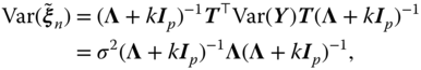
The variance–covariance matrix of is given by

(1.6)

Summation of the diagonal elements of the variance–covariance matrix of is equal to . Apparently, small eigenvalues inflate the total variance of estimate or energy of . Specifically, since the eigenvalues are ordered, if the first eigenvalue is small, it causes the variance to explode. If this happens, what must one do? In the following section, we consider this problem. Therefore, it is of interest to realize when the eigenvalues become small.

Before discussing this problem, a very primitive understanding is that if we enlarge the eigenvalues from to , for some positive value, say, , then we can prevent the total variance from exploding. Of course, the amount of recovery depends on the correct choice of the parameter, .

An artificial remedy is to have based on the variance matrix given by

(1.7)

Replacing the eigenvector matrix in (1.5) by this matrix (1.7), we get the and the variance as in (1.8).

(1.8)

which shows

(1.9)

Further, we show that achieving the total variance of is the target.

1.1.1 Multicollinearity Problem

Multicollinearity or collinearity is the existence of near‐linear relationships among the regressors, predictors, or input/exogenous variables. There are terms such as exact, complete and severe, or supercollinearity and moderate collinearity. Supercollinearity indicates that two (or multiple) covariates are linearly dependent, and moderate occurs when covariates are moderately correlated. In the complete collinearity case, the design matrix is not invertible. This case mostly occurs in a high‐dimensional situation (e.g. microarray measure) in which the number of covariates () exceeds the number of samples ().

Moderation occurs when the relationship between two variables depends on a third variable, namely, the moderator. This case mostly happens in structural equation modeling. Although moderate multicollinearity does not cause the mathematical problems of complete multicollinearity, it does affect the interpretation of model parameter estimates. According to Montgomery et al. (2012), if there is no linear relationship between the regressors, they are said to be orthogonal.

Multicollinearity or ill‐conditioning can create inaccurate estimates of the regression coefficients, inflate the standard errors of the regression coefficients, deflate the partial ‐tests for the regression coefficients, give false and nonsignificant ‐values, and degrade the predictability of the model. It also causes changes in the direction of signs of the coefficient estimates. According to Montgomery et al. (2012), there are five sources for multicollinearity: (i) data collection, (ii) physical constraints, (iii) overdefined model, (iv) model choice or specification, and (v) outliers.

There are many studies that well explain the problem of multicollinearity. Since theoretical aspects of ridge regression and related issues are our goal, we refer the reader to Montgomery et al. (2012) for illustrative examples and comprehensive study on the multicollinearity and diagnostic measures such as correlation matrix, eigen system analysis of , known as condition number, or variance decomposition proportion and variance inflation factor (VIF). To end this section, we consider a frequently used example in a ridge regression, namely, the Portland cement data introduced by Woods et al. (1932) from Najarian et al. (2013). This data set has been analyzed by many authors, e.g. Kaciranlar et al. (1999), Kibria (2003), and Arashi et al. (2015). We assemble the data as follows:

(1.10)

The following (see Tables 1.1 and 1.2) is the partial output of linear regression fit to this data using the software SPSS, where we selected Enter as the method.

We display the VIF values to diagnose the multicollinearity problem in this data set. Values greater than 10 are a sign of multicollinearity. Many softwares can be used.

Model			Adjacent	Standard error of the estimate
1	0.991	0.982	0.974	2.446

Coefficient	Standardized coefficient		Significance	VIF
(Constant)		0.891	0.399
	0.607	2.083	0.071	38.496
	0.528	0.705	0.501	254.423
	0.043	0.135	0.896	46.868
	0.160	0.203	0.844	282.513

1.2 Ridge Regression Estimator: Ridge Notion

If the regression coefficients s are unconstrained, then they can explode (become large); this results in high variance. Hence, in order to control the variance, one may regularize the regression coefficients and determine how large the coefficient grows. In other words, one may impose a constraint on them so as not to get unboundedly large or penalized large regression coefficients. One type of constraint is the ridge constraint given by for some positive value . Hence, the minimization of the penalized residual sum of squares (PRSS) is equivalent to solving the following convex optimization problem,

(1.11)

for some positive value .

In general, the PRSS is defined by

(1.12)

Since the PRSS is a convex function w.r.t. , it has a unique solution. Because of the ridge constraint, the solution is termed as the ridge regression estimator (RRE).

To derive the RRE, we solve the following convex optimization problem

(1.13)

where is the PRSS. Solving

w.r.t. gives the RRE,

(1.14)

Here, is the shrinkage (tuning) parameter. Indeed, tunes (controls) the size of the coefficients, and hence regularizes them. As , the RRE simplifies to the LSE. Also, as , the RREs approach zero. Hence, the optimal shrinkage parameter is of interest.

One must note that solving the optimization problem (1.13) is not the only way of yielding the RRE. It can also be obtained by solving a RSS of another data, say augmented data. To be specific, consider the following augmentation approach. Let

(1.15)

Assume the following multiple linear model,

(1.16)

where is an ‐vector of i.i.d. random variables. Then, the LSE of is obtained as

(1.17)

Thus, the LSE of the augmented data is indeed the RRE of the normal data.

1.3 LSE vs. RRE

Indeed, the RRE is proportional to the LSE. Under the orthonormal case, i.e. , the RRE simplifies to

(1.18)

1.4 Estimation of Ridge Parameter

We can observe from Eq. (1.18) that the RRE heavily depends on the ridge parameter . Many authors at different times worked in this area of research and developed and proposed different estimators for . They considered various models such as linear regression, Poisson regression, and logistic regression models. To mention a few, Hoerl and Kennard (1970), Hoerl et al. (1975), McDonald and Galarneau (1975), Lawless and Wang (1976), Dempster et al. (1977), Gibbons (1981), Kibria (2003), Khalaf and Shukur (2005), Alkhamisi and Shukur (2008), Muniz and Kibria (2009), Gruber et al. (2010), Muniz et al. (2012), Mansson et al. (2010), Hefnawy and Farag (2013), Aslam (2014), and Arashi and Valizadeh (2015), and Kibria and Banik (2016), among others.

1.5 Preliminary Test and Stein‐Type Ridge Estimators

In previous sections, we discussed the notion of RRE and how it shrinks the elements of the ordinary LSE. Sometimes, it is needed to shrink the LSE to a subspace defined by , where is a known matrix of full row rank () and is a vector of known constants. It is also termed as constraint or restriction. Such a configuration of the subspace is frequently used in the design of experiments, known as contrasts. Therefore, sometimes shrinking is for two purposes. We refer to this as double shrinking.

In general, unlike the Bayesian paradigm, correctness of the prior information can be tested on the basis of samples through testing vs. a set of alternatives. Following Fisher's recipe, we use the non‐sample information ; if based on the given sample, we accept . In situations where this prior information is correct, an efficient estimator is the one which satisfies this restriction, called the restricted estimator.

To derive the restricted estimator under a multicollinear situation, satisfying the condition , one solves the following convex optimization problem,

(1.21)

where is the vector of Lagrangian multipliers. Grob (2003) proposed the restricted RRE, under a multicollinear situation, by correcting the restricted RRE of Sarkar (1992).

In our case, we consider prior information with the form , which is a test used for checking goodness of fit. Here, the restricted RRE is simply given by , where is the restricted estimator of . Therefore, one uses if rejects and if accepts. Combining the information existing in both estimators, one may follow an approach by Bancroft (1964), to propose the preliminary test RRE given by

(1.22)

where is the indicator function of the set and is the test statistic for testing , and is the upper ‐level critical value from the ‐distribution with degrees of freedom (D.F.) See Judge and Bock (1978) and Saleh (2006) for the test statistic and details.

After some algebra, it can be shown that

(1.23)

where

Then, it is easy to show that

(1.24)

The preliminary test RRE is discrete in nature and heavily dependent on , the level of significance. Hence, a continuous ‐free estimator is desired. Following James and Stein (1961), the Stein‐type RRE is given by

(1.25)

for some . It is shown in Saleh (2006) that the optimal choice of is equal to , .

Note that if , then , which matches with the estimator . However, if , then becomes a negative estimator. In order to obtain the true value, one has to restrict . Hence, one may define the positive‐rule Stein‐type RRE given by

(1.26)

Although these shrinkage RREs are biased, they outperform the RRE, in the mean squared error (MSE) sense. One must note that this superiority is not uniform over the parameter space . According to how much deviates from the origin, the superiority changes. We refer to Saleh (2006) for an extensive overview on this topic and statistical properties of the shrinkage estimators. This type of estimator will be studied in more detail and compared with the RRE in the following chapters.

1.6 High‐Dimensional Setting

In high‐dimensional analysis, the number of variables is greater than the number of observations, . In such situations, is not invertible and, hence, to derive the LSE of , one may use the generalized inverse of , which does not give a unique solution. However, the RRE can be obtained, regardless of the relationship between and . In this section, we briefly mention some related endeavors in manipulating the RRE to adapt with high‐dimensional setting. However, in Chapter 11, we discuss the growing dimension, i.e. when the sample size is fixed.

Wang et al. (2016) used this fact and proposed a new approach in high‐dimensional regression by considering

(1.27)

They used an orthogonal projection of onto the row space of and proposed the following high‐dimensional version of the LSE for dimension reduction:

(1.28)

They applied the following identity to obtain the estimator:

(1.29)

for every . Buhlmann et al. (2014) also used the projection of onto the row space of and developed a bias correction in the RRE to propose a bias‐corrected RRE for the high‐dimensional setting. Shao and Deng (2012) considered the RRE of the projection vector and proposed to threshold the RRE when the projection vector is sparse, in the sense that many of its components are small.

Specifically, write the SVD of as where and are column orthogonal matrices, and let , , be the eigenvalue matrix corresponding to . Let

(1.30)

where is the projection of onto the row space of .

Since , we have . Obviously, yields as the underlying model instead of (1.1). Then, the RRE of the projection is simply

(1.31)

where is an appropriately chosen regularization parameter.

Shao and Deng (2012) proved that the RRE is consistent for the estimation of any linear combination of ; however, it is not consistent, i.e. may not converge to zero. Then, they proposed an ‐consistent RRE by thresholding.

Another approach to deal with high‐dimensional data in the case is to partition the vector of regression parameters to main and nuisance effects, where we have (say) less than , main and active coefficients that must be estimated and , redundant coefficients that can be eliminated from the analysis by a variable selection method. In fact, we assume some level of sparsity in our inference. Hence, we partition in such a way in which is a vector of main effects and is a vector of nuisance effects. We further assume that . Accordingly, we have the partition for the design matrix. Then, the multiple linear model (1.1) is rewritten as

(1.32)

This model may be termed as the full model. As soon as a variable selection method is used and main effects are selected, the sub model has the form

(1.33)

Then, the interest is to estimate the main effects, (this technique is discussed in more detail in Chapter 11). Therefore, one needs a variable selection method. Unlike the RRE that only shrinks the coefficients, there are many estimators which simultaneously shrink and select variables in large and small problems. The most well‐known one is the least absolute shrinkage and selection operator (LASSO) proposed by Tibshirani (1996). He suggested using an absolute‐type constraint with form for some positive values in the minimization of the PRSS rather than the ridge constraint. Specifically, he defined the PRSS by

(1.34)

where and is an ‐tuple of 1's. The LASSO estimator, denoted by , is the solution to the following convex optimization problem,

(1.35)

To see some recent related endeavors in the context of ridge regression, we refer to Yuzbasi and Ahmed (2015) and Aydin et al. (2016) among others.

In the following section, some of the most recent important references about ridge regression and related topics are listed for more studies.

1.7 Notes and References

The first paper on ridge analysis was by Hoerl (1962); however, the first paper on multicollinearity appeared five years later, roughly speaking, by Farrar and Glauber (1967). Marquardt and Snee (1975) reviewed the theory of ridge regression and its relation to generalized inverse regression. Their study includes several illustrative examples about ridge regression. For the geometry of multicollinearity, see Akdeniz and Ozturk (1981). We also suggest that Gunst (1983) and and Sakallioglu and Akdeniz (1998) not be missed. Gruber (1998) in his monograph motivates the need for using ridge regression and allocated a large portion to the analysis of ridge regression and its generalizations. For historical survey up to 1998, we refer to Gruber (1998).

Beginning from 2000, a comprehensive study in ridge regression is the work of Ozturk and Akdeniz (2000), where the authors provide some solutions for ill‐posed inverse problems. Wan (2002) incorporated measure of goodness of fit in evaluating the RRE and proposed a feasible generalized RRE. Kibria (2003) gave a comprehensive analysis about the estimation of ridge parameter for the linear regression model. For application of ridge regression in agriculture, see Jamal and Rind (2007). Maronna (2011) proposed an RRE based on repeated M‐estimation in robust regression. Saleh et al. (2014) extensively studied the performance of preliminary test and Stein‐type ridge estimators in the multivariate‐t regression model. Huang et al. (2016) defined a weighted VIF for collinearity diagnostic in generalized linear models.

Arashi et al. (2017) studied the performance of several ridge parameter estimators in a restricted ridge regression model with stochastic constraints. Asar et al. (2017) defined a restricted RRE in the logistic regression model and derived its statistical properties. Roozbeh and Arashi (2016a) developed a new ridge estimator in partial linear models. Roozbeh and Arashi (2016b) used difference methodology to study the performance of an RRE in a partial linear model. Arashi and Valizadeh (2015) compared several estimators for estimating the biasing parameter in the study of partial linear models in the presence of multicollinearity. Roozbeh and Arashi (2013) proposed a feasible RRE in partial linear models and studied its properties in details. Roozbeh et al. (2012) developed RREs in seemingly partial linear models. Recently, Chandrasekhar et al. (2016) proposed the concept of partial ridge regression, which involves selectively adjusting the ridge constants associated with highly collinear variables to control instability in the variances of coefficient estimates. Norouzirad and Arashi (2017) developed shrinkage ridge estimators in the context of robust regression. Fallah et al. (2017) studied the asymptotic performance of a general form of shrinkage ridge estimator. Recently, Norouzirad et al. (2017) proposed improved robust ridge M‐estimators and studied their asymptotic behavior.

1.8 Organization of the Book

This book has 12 chapters including this one. In this light we consider the chapter with location and simple linear model first. Chapter 1 presents an introduction to ridge regression and different aspects of it, stressing the multicollinearity problem and its application to high‐dimensional problems. Chapter 2 considers simple linear and location models, and provides theoretical developments. Chapters 3 and 4 deal with the analysis of variance (ANOVA) model and seemingly unrelated simple linear models, respectively. Chapter 5 considers ridge regression and LASSO for multiple regression together with preliminary test and Stein‐type estimator and a comparison thereof when the design matrix is non‐orthogonal. Chapter 6 considers the RRE and its relation to LASSO. Further, we study in detail the properties of the preliminary test and Stein‐type estimator with low dimension. In Chapter 7, we cover the partially linear model and the properties of LASSO, ridge, preliminary test, and the Stein‐type estimators. Chapter 8 contains the discussion on the logistic regression model and the related estimators of diverse kinds as described in earlier chapters. Chapter 9 discusses the multiple regression model with autoregressive errors. In Chapter 10, we provide a comparative study of LASSO, ridge, preliminary test, and Stein‐type estimators using rank‐based theory. In Chapter 11, we discuss the estimation of parameters of a regression model with high dimensions. Finally, we conclude the book with Chapter 12 to illustrate recent applications of ridge, LASSO, and logistic regression to neural networks and big data analysis.