9
Regression Models with Autoregressive Errors
9.1 Introduction
One of the important assumptions of the linear model is that observed responses of the model are independent. However, in reality, significant serial correlation might occur when data are collected sequentially in time. Autocorrelation, also known as serial correlation, occurs when successive items in a series are correlated so that their covariance is not zero and they are not independent. The main objective of this chapter is to develop some penalty and improved estimators, namely, ridge regression estimator (RRE) and the least absolute shrinkage and selection operator (LASSO) and the Stein‐type estimators for the linear regression model with AR(1) errors when some of the coefficients are not statistically significant.
To describe the problem of autocorrelation, we consider the following regression model,
where ![]() 's are
's are ![]() responses,
responses, ![]() is a
is a ![]() known vector of regressors,
known vector of regressors, ![]() is an unknown
is an unknown ![]() vector of unknown regression parameters, and
vector of unknown regression parameters, and ![]() is an
is an ![]() disturbance vector.
disturbance vector.
Under the assumption of independence and ![]() is of full rank, the errors are not autocorrelated and
is of full rank, the errors are not autocorrelated and ![]() and
and ![]() are independently distributed. In that case, the least squares estimator (LSE) of
are independently distributed. In that case, the least squares estimator (LSE) of ![]() is obtained as
is obtained as
with the covariance matrix of ![]() as
as
In a real‐life situation, the necessary assumptions for the LSE may not be met. That means, both regressors and responses may be correlated instead of independent. In that case, the LSE does not possess the optimum property.
Now we will assume that the errors of the model (9.1) has an AR error term of order 1. That is
where ![]() is the autoregressive parameter and
is the autoregressive parameter and ![]() are independently and identically distributed white noise random variables with zero mean and
are independently and identically distributed white noise random variables with zero mean and ![]() variance. The variance covariance matrix of
variance. The variance covariance matrix of ![]() is
is
where

This ![]() matrix is function of AR parameters
matrix is function of AR parameters ![]() and
and ![]() , which need to be estimated from data.
, which need to be estimated from data.
Since the covariance matrix of ![]() is nonspherical, the LSE of
is nonspherical, the LSE of ![]() will be inefficient compared to generalized least squares estimator (GLSE). Thus we need to estimate the parameters using the GLSE. The GLSE of
will be inefficient compared to generalized least squares estimator (GLSE). Thus we need to estimate the parameters using the GLSE. The GLSE of ![]() is
is
with covariance matrix
where

and ![]() is a parameter and can be estimated using the least squares principle as
is a parameter and can be estimated using the least squares principle as

Here, ![]() is the
is the ![]() th residual and
th residual and ![]() , where
, where
and
Now, we are interested in the estimation of subvector ![]() when one suspects from previous studies/experiences that
when one suspects from previous studies/experiences that ![]() is also equal to zero. As such, consider the partition of
is also equal to zero. As such, consider the partition of ![]() , where
, where ![]() and
and ![]() have dimensions
have dimensions ![]() and
and ![]() , respectively, and
, respectively, and ![]() and
and ![]() . Then, we may write the estimators of
. Then, we may write the estimators of ![]() as
as

If we suspect sparsity in ![]() , i.e.
, i.e. ![]() , then the estimator of
, then the estimator of ![]() is given by
is given by

where
9.1.1 Penalty Estimators
We consider two basic penalty estimators, namely, (i) RREs and the (ii) LASSO estimator of ![]() .
.
As for the RREs, we ![]() , yielding a normal equation as
, yielding a normal equation as
so that the RRE of ![]() is obtained as
is obtained as

with the covariance matrix of ![]()

Here, both parameters ![]() and
and ![]() are unknown and need to be estimated from data. RRE for the autoregressive model has been considered by several researchers such as Ismail and Suvarna (2016). To obtain the RRE of
are unknown and need to be estimated from data. RRE for the autoregressive model has been considered by several researchers such as Ismail and Suvarna (2016). To obtain the RRE of ![]() , we consider the asymptotic marginal distribution of
, we consider the asymptotic marginal distribution of

where

respectively, with

Also,

and

From (9.9), we define the RREs of ![]() as
as

9.1.2 Shrinkage Estimators
9.1.2.1 Preliminary Test Estimator
Since, we suspect that the sparsity condition, ![]() , may hold, we use the Wald test statistic,
, may hold, we use the Wald test statistic, ![]() , for testing the hypothesis
, for testing the hypothesis ![]() , where
, where

For large samples and under ![]() ,
, ![]() has a chi‐square distribution with
has a chi‐square distribution with ![]() degrees of freedom (D.F.) Let
degrees of freedom (D.F.) Let ![]() , (say) be the
, (say) be the ![]() ‐level critical value from the null distribution of
‐level critical value from the null distribution of ![]() . Then, the preliminary test estimator (PTE) of
. Then, the preliminary test estimator (PTE) of ![]() may be written using the marginal distribution of
may be written using the marginal distribution of ![]() as
as

where ![]() is the indicator function of the set
is the indicator function of the set ![]() .
.
9.1.2.2 Stein‐Type and Positive‐Rule Stein‐Type Estimators
We notice that PTE is a discrete function and loses some optimality properties. Thus, we consider the continuous version of the PTE which mimics the Stein‐type estimators given by

Since the SE may yield estimators with wrong signs, we consider the positive‐rule Stein‐type estimator (PRSE) of ![]() given by
given by

9.1.3 Results on Penalty Estimators
A modified least absolute shrinkage and selection operator (MLASSO) estimator may be defined by the vector

where ![]() is the
is the ![]() th diagonal element of
th diagonal element of ![]() . This estimator puts some coefficient exactly equal to zero.
. This estimator puts some coefficient exactly equal to zero.
Now, we know that the asymptotic marginal distribution of
We consider the estimation of ![]() by any estimator
by any estimator ![]() under the
under the ![]() ‐risk function
‐risk function
Consider the family of diagonal linear projections
Following Chapter 08, we obtain the ideal ![]() risk
risk

Now, if ![]() coefficients exceed the noise level and
coefficients exceed the noise level and ![]() coefficients are 0's, then the
coefficients are 0's, then the ![]() risk is given by
risk is given by
Consequently, the weighted ![]() ‐risk lower bound is given by
‐risk lower bound is given by ![]() as
as

We shall use this lower bound to compare MLASSO with other estimators. For details on LASSO estimators, see Chapter 05.
9.1.4 Results on PTE and Stein‐Type Estimators
In this section, we present the asymptotic distributional bias (ADB) and asymptotic distributional ![]() ‐risk (ADR) of the shrinkage estimators.
‐risk (ADR) of the shrinkage estimators.
9.1.5 Results on Penalty Estimators
First, we consider the simplest version of the RRE given by

The risk function for RRE is

The weighted ![]() ‐risk function is
‐risk function is

The optimum value of ![]() is obtained as
is obtained as ![]() . So that
. So that

The risk function of the MLASSO estimator is
The weighted ![]() ‐risk function is
‐risk function is
9.2 Asymptotic Distributional  ‐risk Efficiency Comparison
In this section, we study the comparative properties of the estimators relative to the GLSEs. We consider the weighted ![]() ‐risk to compare the performance of the estimators. However, it is noted that all of the weighted
‐risk to compare the performance of the estimators. However, it is noted that all of the weighted ![]() ‐risk functions in this chapter except for the restricted LSEs are identical to those of the
‐risk functions in this chapter except for the restricted LSEs are identical to those of the ![]() risk functions in Chapter 08. Thus, we should skip the finite sample comparison among the estimators except for the RGLSE.
risk functions in Chapter 08. Thus, we should skip the finite sample comparison among the estimators except for the RGLSE.
9.2.1 Comparison of GLSE with RGLSE
In this case, the asymptotic distributional relative weighted ![]() ‐risk efficiency of RGLSE vs. GLSE is given by
‐risk efficiency of RGLSE vs. GLSE is given by

where
The ![]() is a decreasing function of
is a decreasing function of ![]() . At
. At ![]() , its value is
, its value is

and as ![]() , its value is 0. It crosses the 1‐line at
, its value is 0. It crosses the 1‐line at ![]() . So,
. So,

In order to compute ![]() , we need to find
, we need to find ![]() ,
, ![]() , and
, and ![]() . These are obtained by generating explanatory variables by the following equation based on McDonald and Galarneau (1975),
. These are obtained by generating explanatory variables by the following equation based on McDonald and Galarneau (1975),
where ![]() are independent
are independent ![]() pseudorandom numbers and
pseudorandom numbers and ![]() is the correlation between any two explanatory variables. In this study, we take
is the correlation between any two explanatory variables. In this study, we take ![]() , and 0.9 which shows the variables are lightly collinear and severely collinear. In our case, we chose
, and 0.9 which shows the variables are lightly collinear and severely collinear. In our case, we chose ![]() and various
and various ![]() . The resulting output is then used to compute
. The resulting output is then used to compute ![]() .
.
9.2.2 Comparison of GLSE with PTE
Here, the relative weighted ![]() ‐risk efficiency expression for PTE vs. LSE is given by
‐risk efficiency expression for PTE vs. LSE is given by

where
Then, the PTE outperforms the LSE for

Otherwise, LSE outperforms the PTE in the interval ![]() . We may mention that
. We may mention that ![]() is a decreasing function of
is a decreasing function of ![]() with a maximum at the point
with a maximum at the point ![]() , then decreases crossing the 1‐line to a minimum at the point
, then decreases crossing the 1‐line to a minimum at the point ![]() with a value
with a value ![]() , and then increases toward 1‐line.
, and then increases toward 1‐line.
The ![]() belongs to the interval
belongs to the interval

where ![]() depends on the size
depends on the size ![]() and given by
and given by

The quantity ![]() is the value
is the value ![]() at which the relative weighted
at which the relative weighted ![]() ‐risk efficiency value is minimum.
‐risk efficiency value is minimum.
9.2.3 Comparison of LSE with SE and PRSE
Since SE and PRSE need ![]() to express their weighted
to express their weighted ![]() ‐risk expressions, we assume always
‐risk expressions, we assume always ![]() . We have
. We have

It is a decreasing function of ![]() . At
. At ![]() , its value is
, its value is ![]() and when
and when ![]() , its value goes to 1. Hence, for
, its value goes to 1. Hence, for ![]() ,
,

Also,

So that,
9.2.4 Comparison of LSE and RLSE with RRE
First, we consider weighted ![]() ‐risk difference of GLSE and RRE given by
‐risk difference of GLSE and RRE given by

Hence, RRE outperforms the GLSE uniformly. Similarly, for the RGLSE and RRE, the weighted ![]() ‐risk difference is given by
‐risk difference is given by

If ![]() , then 9.63 is negative. Hence, RGLSE outperforms RRE at this point. Solving the equation
, then 9.63 is negative. Hence, RGLSE outperforms RRE at this point. Solving the equation

for ![]() , we get
, we get

If ![]() , RGLSE outperforms better than the RRE, and if
, RGLSE outperforms better than the RRE, and if ![]() , RRE performs better than RGLSE; Thus, RGLSE nor RRE outperforms the other uniformly.
, RRE performs better than RGLSE; Thus, RGLSE nor RRE outperforms the other uniformly.
In addition, the relative weighted ![]() ‐risk efficiency of RRE vs. GLSE equals
‐risk efficiency of RRE vs. GLSE equals

which is a decreasing function of ![]() with maximum
with maximum ![]() at
at ![]() and minimum 1 as
and minimum 1 as ![]() . So,
. So,

9.2.5 Comparison of RRE with PTE, SE and PRSE
9.2.5.1 Comparison Between  and
and 
Here, the weighted ![]() ‐risk difference of
‐risk difference of ![]() and
and ![]() is given by
is given by

Note that the risk of ![]() is an increasing function of
is an increasing function of ![]() crossing the
crossing the ![]() ‐line to a maximum and then drops monotonically toward the
‐line to a maximum and then drops monotonically toward the ![]() ‐line as
‐line as ![]() . The value of the risk is
. The value of the risk is ![]() at
at ![]() . On the other hand,
. On the other hand, ![]() is an increasing function of
is an increasing function of ![]() below the
below the ![]() ‐line with a minimum value 0 at
‐line with a minimum value 0 at ![]() and as
and as ![]() ,
, ![]() . Hence, the risk difference in Eq. 9.67 is nonnegative for
. Hence, the risk difference in Eq. 9.67 is nonnegative for ![]() . Thus, the RRE uniformly performs better than PTE.
. Thus, the RRE uniformly performs better than PTE.
9.2.5.2 Comparison Between  and
and 
The weighted ![]() ‐risk difference of
‐risk difference of ![]() and
and ![]() is given by
is given by

Note that the first function is increasing in ![]() with a value
with a value ![]() at
at ![]() ; and as
; and as ![]() , it tends to
, it tends to ![]() . The second function is also increasing in
. The second function is also increasing in ![]() with a value
with a value ![]() at
at ![]() and approaches the value
and approaches the value ![]() as
as ![]() . Hence, the risk difference is nonnegative for all
. Hence, the risk difference is nonnegative for all ![]() . Consequently, RRE outperforms SE uniformly.
. Consequently, RRE outperforms SE uniformly.
9.2.5.3 Comparison of  with
with 
The ![]() risk of
risk of ![]() is
is
where

and ![]() is
is
The weighted ![]() ‐risk difference of PRSE and RRE is given by
‐risk difference of PRSE and RRE is given by

where

Consider the ![]() . It is a monotonically increasing function of
. It is a monotonically increasing function of ![]() . At
. At ![]() , its value is
, its value is ![]() ; and as
; and as ![]() , it tends to
, it tends to ![]() . For
. For ![]() , at
, at ![]() , the value is
, the value is ![]() ; and as
; and as ![]() , it tends to
, it tends to ![]() . Hence, the
. Hence, the ![]() ‐risk difference in 9.71 is nonnegative and RRE uniformly outperforms PRSE.
‐risk difference in 9.71 is nonnegative and RRE uniformly outperforms PRSE.
Note that the risk difference of ![]() and
and ![]() at
at ![]() is
is

because the expected value in Eq. 9.72 is a decreasing function of D.F., and
9.2.6 Comparison of MLASSO with GLSE and RGLSE
First, note that if ![]() coefficients
coefficients ![]() and
and ![]() coefficients are zero in a sparse solution, the lower bound of the weighted
coefficients are zero in a sparse solution, the lower bound of the weighted ![]() risk is given by
risk is given by ![]() . Thereby, we compare all estimators relative to this quantity. Hence, the weighted
. Thereby, we compare all estimators relative to this quantity. Hence, the weighted ![]() ‐risk difference between LSE and MLASSO is given by
‐risk difference between LSE and MLASSO is given by
Hence, if ![]() , the MLASSO performs better than the LSE, while if
, the MLASSO performs better than the LSE, while if ![]() the LSE performs better than the MLASSO. Consequently, neither LSE nor the MLASSO performs better than the other uniformly.
the LSE performs better than the MLASSO. Consequently, neither LSE nor the MLASSO performs better than the other uniformly.
Next we compare the RGLSE and MLASSO. In this case, the weighted ![]() ‐risk difference is given by
‐risk difference is given by
Hence, the RGLSE uniformly performs better than the MLASSO. If ![]() , MLASSO and RGLSE are
, MLASSO and RGLSE are ![]() ‐risk equivalent. If the GLSEs are independent, then
‐risk equivalent. If the GLSEs are independent, then ![]() . Hence, MLASSO satisfies the oracle properties.
. Hence, MLASSO satisfies the oracle properties.
9.2.7 Comparison of MLASSO with PTE, SE, and PRSE
We first consider the PTE vs. MLASSO. In this case, the weighted ![]() ‐risk difference is given by
‐risk difference is given by

Hence, the MLASSO outperforms the PTE when ![]() . But, when
. But, when ![]() , then the MLASSO outperforms the PTE for
, then the MLASSO outperforms the PTE for

Otherwise, PTE outperforms the MLASSO. Hence, neither PTE nor MLASSO outperforms the other uniformly.
Next, we consider SE and PRSE vs. the MLASSO. In these two cases, we have weighted ![]() ‐risk differences given by
‐risk differences given by

and from 9.69,

where ![]() is given by 9.70. Hence, the MLASSO outperforms the SE as well as the PRSE in the interval
is given by 9.70. Hence, the MLASSO outperforms the SE as well as the PRSE in the interval
Thus, neither the SE nor the PRSE outperforms the MLASSO, uniformly.
9.2.8 Comparison of MLASSO with RRE
Here, the weighted ![]() ‐risk difference is given by
‐risk difference is given by

Hence, the RRE outperforms the MLASSO uniformly.
9.3 Example: Sea Level Rise at Key West, Florida
In this section, we want to illustrate the methodology of this chapter by using a real data application. In this regard, we want to see whether there is any relationship between sea level rise at Key West, Florida with the following regressors: time (year); atmospheric carbon dioxide concentration (![]() ); ocean heat content (OHC); global mean temperature (Temp); RF; PC; sunspots (SP); Pacific decadal oscillation (PDO); Southern Oscillation Index (SOI), which measures the strength of the Southern Oscillation.
); ocean heat content (OHC); global mean temperature (Temp); RF; PC; sunspots (SP); Pacific decadal oscillation (PDO); Southern Oscillation Index (SOI), which measures the strength of the Southern Oscillation.
The sources of data are: (i) National Oceanographic and Atmospheric Administration (NOAA), (ii) Australian Government Bureau of Meteorology, and (iii) NASA Goddard Institute for Space Studies (NASA GISS). Since there are a lot of missing values and some variables are measured at a later time, we consider data between 1959 and 2016 so that we can consider nine (9) independent variables (regressors). All variables are standardized so that all regression coefficients are comparable.
We consider the following linear regression model:

We first apply the LSE and fit the following linear regression model:

with ![]() ,
, ![]() , and
, and ![]() with
with ![]() and
and ![]() ‐value =
‐value = ![]() . This indicates that overall the regression model is significant.
. This indicates that overall the regression model is significant.
The correlation matrix among the variables is given in Table 9.1. If we review Table 9.1, we can see that there are moderate to strong relationships among some of the regressors.
Table 9.1 Correlation coefficients among the variables.
| SL | OHC | Year | Temp | RF | PC | SP | PDO | SOI | ||
| SL | 1.000 | 0.894 | 0.846 | 0.885 | 0.828 | |||||
| 0.894 | 1.000 | 0.952 | 0.993 | 0.920 | 0.010 | 0.008 | ||||
| OHC | 0.846 | 0.952 | 1.000 | 0.920 | 0.912 | 0.020 | ||||
| Year | 0.885 | 0.993 | 0.920 | 1.000 | 0.898 | 0.008 | 0.012 | |||
| Temp | 0.828 | 0.920 | 0.912 | 0.898 | 1.000 | 0.080 | 0.063 | |||
| RF | 0.010 | 0.008 | 0.080 | 1.000 | 0.967 | 0.119 | 0.045 | |||
| PC | 0.008 | 0.012 | 0.063 | 0.967 | 1.000 | 0.121 | 0.025 | |||
| SP | 0.119 | 0.121 | 1.000 | 0.002 | ||||||
| PDO | 0.045 | 0.025 | 0.002 | 1.000 | ||||||
| SOI | 0.020 | 1.000 |
9.3.1 Estimation of the Model Parameters
9.3.1.1 Testing for Multicollinearity
We can see from Table 9.2 that among the nine regressors, six have variance inflation factor (VIF) greater than 10. So there is moderate to strong multicollinearity existing in the data.
Table 9.2 VIF values related to sea level rise at Key West, Florida data set.
| Variables | VIF |
| 239.285 | |
| OHC | 21.678 |
| Year | 139.294 |
| Temp | 9.866 |
| RF | 16.371 |
| PC | 16.493 |
| SP | 1.135 |
| PDO | 1.624 |
| SOI | 1.877 |
Condition index: ![]() . Since the condition number exceeds 1000, we may conclude that at least one of the regressors is responsible for the multicollinearity problem in the data.
. Since the condition number exceeds 1000, we may conclude that at least one of the regressors is responsible for the multicollinearity problem in the data.
Thus, from the correlation matrix, VIF, and the condition number, we conclude that these data suffer from the problem of multicollinearity.
9.3.1.2 Testing for Autoregressive Process
Using the following R command, we found that the residual of the model follow AR(1) process. The estimated AR(1) coefficient, ![]() .
.
> phi=Arima(Res, order=c(1,1,0))$coe> phiar1---0.3343068
Since the data follow AR(1) process and the regressors are correlated, this data will be the most appropriate to analyze for this chapter.
9.3.1.3 Estimation of Ridge Parameter 
Following Kibria (2003) and Kibria and Banik (2016), we may estimate the ridge coefficient ![]() . However, since different methods produce different values of
. However, since different methods produce different values of ![]() , we consider the
, we consider the
> rstats2(ridge1.lm)$PRESSK=0.001 K=0.01 K=0.05 K=0.1 K=0.5 K=0.9 K=115.40242 15.26157 14.80704 14.59746 14.82246 15.82000 16.12388
We use ![]() because this value gives a smaller predicted residual error sum of squares (PRESS).
because this value gives a smaller predicted residual error sum of squares (PRESS).
Based on the full fitted model, we consider the following hypotheses:
![]() and
and ![]() . We test the following hypothesis,
. We test the following hypothesis,
where
The fitted reduced linear regression model is
Now, using ![]() , and
, and ![]() , the estimated values of the regression coefficient are provided in Table 9.3.
, the estimated values of the regression coefficient are provided in Table 9.3.
Table 9.3 Estimation of parameter using different methods (![]() ,
, ![]() ,
, ![]() , and
, and ![]() ).
).
| GLSE | RGLSEE | RRE | MLASSO | PTGLSE | SGLSE | PRSLSE | |
| 2.533 | 2.533 | 2.533 | 2.533 | 2.533 | 2.533 | 2.533 | |
| OHC | 0.000 | ||||||
| Year | 0.000 | ||||||
| Temp | 0.208 | 0.208 | 0.198 | 0.000 | 0.208 | 0.178 | 0.178 |
| RF | 0.046 | 0.046 | 0.044 | 0.000 | 0.046 | 0.039 | 0.039 |
| PC | 0.021 | 0.021 | 0.020 | 0.000 | 0.021 | 0.018 | 0.018 |
| SP | 0.000 | ||||||
| PDO | 0.000 | ||||||
| SOI | 0.000 |
If we review Table 9.3, we can see that LASSO kept variable ![]() and kicked out the rest of the regressors. The sign of the temperature has been changed from negative to positive. This is true because as the temperature go up, the sea level should go up too. Table 9.4 also indicates that the LSE gave the wrong sign for the temperature variable and only
and kicked out the rest of the regressors. The sign of the temperature has been changed from negative to positive. This is true because as the temperature go up, the sea level should go up too. Table 9.4 also indicates that the LSE gave the wrong sign for the temperature variable and only ![]() is marginally significant at 5% significance level.
is marginally significant at 5% significance level.
Table 9.4 Estimation of parameter using LSE (![]() ,
, ![]() ,
, ![]() , and
, and ![]() ).
).
| LSE | Standard error | Pr( |
||
| Intercept | ||||
| 1.903 | 0.960 | 1.982 | 0.0532 | |
| OHC | 0.521 | |||
| Year | 0.285 | |||
| Temp | 0.195 | 0.8033 | ||
| RF | 0.251 | 0.286 | ||
| PC | 0.215 | 0.252 | 0.856 | 0.396 |
| SP | 0.061 | 0.677 | ||
| PDO | 0.079 | 0.916 | ||
| SOI | 0.085 | 0.247 |
Now, we consider the relative efficiency (REff) criterion to compare the performance of the estimators.
9.3.2 Relative Efficiency
9.3.2.1 Relative Efficiency (REff)
The REff of ![]() compared to GLSE is defined as
compared to GLSE is defined as

where ![]() could be any of the proposed estimators. If we review the risk functions (except GLSE) under Theorem 9.1.1, all the terms contain
could be any of the proposed estimators. If we review the risk functions (except GLSE) under Theorem 9.1.1, all the terms contain ![]() . To write these risk functions in terms of
. To write these risk functions in terms of ![]() , we adopt the following procedure.
, we adopt the following procedure.
We obtain from Anderson (1984, Theorem A.2.4, p. 590) that

Since, ![]() , the above equation can be written as
, the above equation can be written as
where ![]() and
and ![]() are, respectively, the largest and the smallest characteristic roots of the matrix,
are, respectively, the largest and the smallest characteristic roots of the matrix, ![]() . Using this result, the risk functions can be written as follows:
. Using this result, the risk functions can be written as follows:
The risk function for GLSE is
The risk function for RGLSE is
The risk of PTGLSE is

The risk function for SGLSE is

The risk function of PRSGLSE is

The risk function for generalized RRE is

The risk function of MLASSO is
Using the risk functions in 9.84–9.90, the REff of the estimators for different values of ![]() are given in Table 9.5.
are given in Table 9.5.
Table 9.5 Relative efficiency of the proposed estimators (![]() ,
, ![]() ,
, ![]() , and
, and ![]() ).
).
| GLSE | RGLSE | RRE | MLASSO | PTGLSE | SGLSE | PRSGLSE | |
| 0.000 | 1.000 | 2.605 | 1.022 | 1.144 | 0.815 | 1.099 | 1.177 |
| 0.100 | 1.000 | 2.512 | 1.022 | 1.125 | 0.806 | 1.087 | 1.164 |
| 0.500 | 1.000 | 2.198 | 1.022 | 1.058 | 0.776 | 1.045 | 1.115 |
| 1.000 | 1.000 | 1.901 | 1.021 | 0.984 | 0.743 | 1.004 | 1.066 |
| 2.000 | 1.000 | 1.497 | 1.020 | 0.863 | 0.690 | 0.947 | 0.995 |
| 5.000 | 1.000 | 0.914 | 1.016 | 0.631 | 0.612 | 0.871 | 0.893 |
| 10.000 | 1.000 | 0.554 | 1.010 | 0.436 | 0.626 | 0.849 | 0.855 |
| 15.000 | 1.000 | 0.398 | 1.004 | 0.333 | 0.726 | 0.857 | 0.858 |
| 20.000 | 1.000 | 0.310 | 0.998 | 0.269 | 0.841 | 0.870 | 0.870 |
| 25.000 | 1.000 | 0.254 | 0.993 | 0.226 | 0.926 | 0.882 | 0.882 |
| 30.000 | 1.000 | 0.215 | 0.987 | 0.195 | 0.971 | 0.893 | 0.893 |
| 40.000 | 1.000 | 0.165 | 0.975 | 0.153 | 0.997 | 0.911 | 0.911 |
| 50.000 | 1.000 | 0.134 | 0.964 | 0.125 | 1.000 | 0.923 | 0.923 |
| 60.000 | 1.000 | 0.112 | 0.954 | 0.106 | 1.000 | 0.933 | 0.933 |
| 100.000 | 1.000 | 0.069 | 0.913 | 0.066 | 1.000 | 0.999 | 0.999 |
The relative efficiencies of the estimators for different values of ![]() are given in Figure 9.1 and Table 9.6.
are given in Figure 9.1 and Table 9.6.
If we review Tables 9.5 and 9.6, we can see that the performance of the estimators except the GLSE depend on the values of ![]() ,
, ![]() ,
, ![]() ,
, ![]() , and
, and ![]() . We immediately see that the restricted estimator outperforms all the estimators when the restriction is at 0. However, as
. We immediately see that the restricted estimator outperforms all the estimators when the restriction is at 0. However, as ![]() goes away from the null hypothesis, the REff of RGLSE goes down and performs the worst when
goes away from the null hypothesis, the REff of RGLSE goes down and performs the worst when ![]() is large. Both PRSGLSE and SGLSE uniformly dominate the RRE and MLASSO estimator. We also observe that the GLSE uniformly dominates the PTGLSE for
is large. Both PRSGLSE and SGLSE uniformly dominate the RRE and MLASSO estimator. We also observe that the GLSE uniformly dominates the PTGLSE for ![]() . The REff of PTGLSE increases as
. The REff of PTGLSE increases as ![]() increases. These conclusions looks unusual, probably due to autocorrelated data. However, when
increases. These conclusions looks unusual, probably due to autocorrelated data. However, when ![]() is large, we have the usual conclusions (see Tables 9.7 and 9.8).
is large, we have the usual conclusions (see Tables 9.7 and 9.8).

Figure 9.1 Relative efficiency of the estimators for  ,
,  ,
,  , and
, and  .
.
9.3.2.2 Effect of Autocorrelation Coefficient 
To see the effect of the autocorrelation coefficient ![]() on the performance of the proposed shrinkage, LASSO and RREs, we evaluated the REff for various values of
on the performance of the proposed shrinkage, LASSO and RREs, we evaluated the REff for various values of ![]() , and 0.75 and presented them, respectively, in Figures 9.2–9.4 and Tables 9.6–9.9. If we review these figures and tables, under
, and 0.75 and presented them, respectively, in Figures 9.2–9.4 and Tables 9.6–9.9. If we review these figures and tables, under ![]() , we observe that the RGLSE performed the best followed by PRSGLSE, LASSO, SGLSE, and RRE; and PTGLSE (with
, we observe that the RGLSE performed the best followed by PRSGLSE, LASSO, SGLSE, and RRE; and PTGLSE (with ![]() ) performed the worst. The performance of the RGLSE becomes worse when
) performed the worst. The performance of the RGLSE becomes worse when ![]() increases and becomes inefficient for large
increases and becomes inefficient for large ![]() .
.
To see the opposite effect of the autocorrelation coefficient on the proposed estimators, we evaluated the REff of the estimators for ![]() and
and ![]() and presented them in Figures 9.5 and 9.6 and Tables 9.10 and 9.11. If we review these two figures and tables, we can see that the proposed estimators perform better for positive value of
and presented them in Figures 9.5 and 9.6 and Tables 9.10 and 9.11. If we review these two figures and tables, we can see that the proposed estimators perform better for positive value of ![]() than for the negative value of
than for the negative value of ![]() .
.
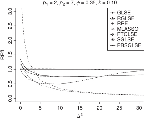
Figure 9.2 Relative efficiency of the estimators for  ,
,  ,
,  , and
, and  .
.

Figure 9.3 Relative efficiency of the estimators for  ,
,  ,
,  , and
, and  .
.

Figure 9.4 Relative efficiency of the estimators for  ,
,  ,
,  , and
, and  .
.
Table 9.7 The relative efficiency of the proposed estimators (![]() ,
, ![]() ,
, ![]() , and
, and ![]() ).
).
| GLSE | RGLSE | RRE | MLASSO | PTGLSE | SGLSE | PRSGLSE | |
| 0.000 | 1.000 | 4.334 | 1.056 | 1.279 | 0.989 | 1.185 | 1.355 |
| 0.100 | 1.000 | 3.871 | 1.056 | 1.236 | 0.963 | 1.158 | 1.321 |
| 0.500 | 1.000 | 2.711 | 1.054 | 1.087 | 0.874 | 1.070 | 1.208 |
| 1.000 | 1.000 | 1.973 | 1.051 | 0.945 | 0.787 | 0.990 | 1.104 |
| 2.000 | 1.000 | 1.277 | 1.046 | 0.750 | 0.666 | 0.887 | 0.968 |
| 5.000 | 1.000 | 0.621 | 1.031 | 0.462 | 0.510 | 0.766 | 0.800 |
| 10.000 | 1.000 | 0.334 | 1.006 | 0.282 | 0.494 | 0.736 | 0.744 |
| 15.000 | 1.000 | 0.229 | 0.983 | 0.203 | 0.596 | 0.749 | 0.751 |
| 20.000 | 1.000 | 0.174 | 0.961 | 0.159 | 0.743 | 0.769 | 0.770 |
| 25.000 | 1.000 | 0.140 | 0.940 | 0.130 | 0.871 | 0.789 | 0.789 |
| 30.000 | 1.000 | 0.117 | 0.919 | 0.110 | 0.947 | 0.807 | 0.807 |
| 40.000 | 1.000 | 0.089 | 0.881 | 0.085 | 0.994 | 0.836 | 0.836 |
| 50.000 | 1.000 | 0.071 | 0.846 | 0.069 | 1.000 | 0.858 | 0.858 |
| 60.000 | 1.000 | 0.060 | 0.814 | 0.058 | 1.000 | 0.875 | 0.875 |
| 100.000 | 1.000 | 0.036 | 0.706 | 0.035 | 1.000 | 0.995 | 0.995 |
Table 9.6 The relative efficiency of the proposed estimators (![]() ,
, ![]() ,
, ![]() , and
, and ![]() ).
).
| GLSE | RGLSE | RRE | MLASSO | PTGLSE | SGLSE | PRSGLSE | |
| 0.000 | 1.000 | 1.117 | 1.004 | 1.023 | 0.579 | 1.008 | 1.011 |
| 0.100 | 1.000 | 1.062 | 1.004 | 0.977 | 0.566 | 0.993 | 0.998 |
| 0.500 | 1.000 | 0.889 | 1.002 | 0.828 | 0.523 | 0.944 | 0.956 |
| 1.000 | 1.000 | 0.738 | 1.000 | 0.696 | 0.482 | 0.902 | 0.918 |
| 2.000 | 1.000 | 0.551 | 0.996 | 0.527 | 0.429 | 0.854 | 0.871 |
| 5.000 | 1.000 | 0.313 | 0.985 | 0.305 | 0.386 | 0.825 | 0.834 |
| 10.000 | 1.000 | 0.182 | 0.967 | 0.179 | 0.477 | 0.856 | 0.858 |
| 15.000 | 1.000 | 0.128 | 0.950 | 0.127 | 0.664 | 0.887 | 0.888 |
| 20.000 | 1.000 | 0.099 | 0.933 | 0.098 | 0.843 | 0.909 | 0.909 |
| 25.000 | 1.000 | 0.081 | 0.917 | 0.080 | 0.945 | 0.924 | 0.924 |
| 30.000 | 1.000 | 0.068 | 0.901 | 0.068 | 0.984 | 0.935 | 0.935 |
| 40.000 | 1.000 | 0.052 | 0.871 | 0.052 | 0.999 | 0.949 | 0.949 |
| 50.000 | 1.000 | 0.042 | 0.843 | 0.042 | 1.000 | 0.959 | 0.959 |
| 60.000 | 1.000 | 0.035 | 0.817 | 0.035 | 1.000 | 0.965 | 0.965 |
| 100.000 | 1.000 | 0.021 | 0.727 | 0.021 | 1.000 | 0.996 | 0.996 |
Table 9.8 The relative efficiency of the proposed estimators (![]() ,
, ![]() ,
, ![]() , and
, and ![]() ).
).
| GLSE | RGLSE | RRE | MLASSO | PTGLSE | SGLSE | PRSGLSE | |
| 0.000 | 1.000 | 5.512 | 1.076 | 1.410 | 1.107 | 1.262 | 1.537 |
| 0.100 | 1.000 | 4.829 | 1.076 | 1.361 | 1.076 | 1.234 | 1.492 |
| 0.500 | 1.000 | 3.228 | 1.074 | 1.194 | 0.970 | 1.141 | 1.348 |
| 1.000 | 1.000 | 2.282 | 1.071 | 1.035 | 0.868 | 1.055 | 1.218 |
| 2.000 | 1.000 | 1.439 | 1.066 | 0.818 | 0.728 | 0.945 | 1.052 |
| 5.000 | 1.000 | 0.683 | 1.052 | 0.502 | 0.548 | 0.814 | 0.853 |
| 10.000 | 1.000 | 0.364 | 1.028 | 0.305 | 0.522 | 0.776 | 0.785 |
| 15.000 | 1.000 | 0.248 | 1.005 | 0.219 | 0.619 | 0.784 | 0.786 |
| 20.000 | 1.000 | 0.188 | 0.984 | 0.171 | 0.760 | 0.801 | 0.802 |
| 25.000 | 1.000 | 0.152 | 0.963 | 0.140 | 0.881 | 0.818 | 0.818 |
| 30.000 | 1.000 | 0.127 | 0.943 | 0.119 | 0.951 | 0.834 | 0.834 |
| 40.000 | 1.000 | 0.096 | 0.906 | 0.091 | 0.995 | 0.859 | 0.859 |
| 50.000 | 1.000 | 0.077 | 0.871 | 0.074 | 1.000 | 0.878 | 0.878 |
| 60.000 | 1.000 | 0.064 | 0.840 | 0.062 | 1.000 | 0.893 | 0.893 |

Figure 9.5 Relative efficiency of the estimators for  ,
,  ,
,  , and
, and  .
.

Figure 9.6 Relative efficiency of the estimators for  ,
,  ,
,  , and
, and  .
.
Table 9.9 The relative efficiency of the proposed estimators (![]() ,
, ![]() ,
, ![]() , and
, and ![]() ).
).
| GLSE | RGLSE | RRE | MLASSO | PTGLSE | SGLSE | PRSGLSE | |
| 0.000 | 1.000 | 8.994 | 1.113 | 1.712 | 1.366 | 1.422 | 1.996 |
| 0.100 | 1.000 | 7.887 | 1.112 | 1.667 | 1.335 | 1.401 | 1.933 |
| 0.500 | 1.000 | 5.287 | 1.111 | 1.510 | 1.225 | 1.325 | 1.731 |
| 1.000 | 1.000 | 3.744 | 1.110 | 1.351 | 1.115 | 1.252 | 1.552 |
| 2.000 | 1.000 | 2.364 | 1.106 | 1.116 | 0.956 | 1.150 | 1.330 |
| 5.000 | 1.000 | 1.123 | 1.097 | 0.733 | 0.731 | 1.010 | 1.064 |
| 10.000 | 1.000 | 0.599 | 1.081 | 0.467 | 0.671 | 0.948 | 0.958 |
| 15.000 | 1.000 | 0.408 | 1.066 | 0.342 | 0.743 | 0.936 | 0.938 |
| 20.000 | 1.000 | 0.310 | 1.051 | 0.270 | 0.846 | 0.937 | 0.937 |
| 25.000 | 1.000 | 0.249 | 1.036 | 0.223 | 0.927 | 0.940 | 0.940 |
| 30.000 | 1.000 | 0.209 | 1.022 | 0.190 | 0.971 | 0.945 | 0.945 |
| 40.000 | 1.000 | 0.158 | 0.995 | 0.147 | 0.997 | 0.952 | 0.952 |
| 50.000 | 1.000 | 0.126 | 0.970 | 0.119 | 1.000 | 0.959 | 0.959 |
| 60.000 | 1.000 | 0.106 | 0.945 | 0.101 | 1.000 | 0.964 | 0.964 |
| 100.000 | 1.000 | 0.064 | 0.859 | 0.062 | 1.000 | 1.025 | 1.025 |
9.4 Summary and Concluding Remarks
In this chapter, we considered the multiple linear regression model when the regressors are not independent and errors follow an AR(1) process. We proposed some shrinkage, namely, restricted estimator, PTE, Stein‐type estimator, PRSE as well as penalty estimators, namely, LASSO and RRE for estimating the regression parameters. We obtained the asymptotic distributional ![]() risk of the estimators and compared them in the sense of smaller risk and noncentrality parameter
risk of the estimators and compared them in the sense of smaller risk and noncentrality parameter ![]() . We found that the performance of the estimators depend on the value of the autocorrelation coefficient,
. We found that the performance of the estimators depend on the value of the autocorrelation coefficient, ![]() , number of regressors, and noncentrality parameter
, number of regressors, and noncentrality parameter ![]() . A real‐life data was analyzed to illustrate the performance of the estimators. It is shown that the ridge estimator dominates the rest of the estimators under a correctly specified model. However, it shows poor performance when
. A real‐life data was analyzed to illustrate the performance of the estimators. It is shown that the ridge estimator dominates the rest of the estimators under a correctly specified model. However, it shows poor performance when ![]() moves from the null hypothesis. We also observed that the proposed estimators perform better for a positive value of
moves from the null hypothesis. We also observed that the proposed estimators perform better for a positive value of ![]() than for a negative value of
than for a negative value of ![]() .
.
Table 9.10 The relative efficiency of the proposed estimators (![]() ,
, ![]() ,
, ![]() , and
, and ![]() ).
).
| GLSE | RGLSE | RRE | MLASSO | PTGLSE | SGLSE | PRSGLSE | |
| 0.000 | 1.000 | 14.861 | 1.094 | 1.978 | 1.602 | 1.546 | 2.459 |
| 0.100 | 1.000 | 13.895 | 1.094 | 1.960 | 1.585 | 1.538 | 2.389 |
| 0.500 | 1.000 | 11.028 | 1.094 | 1.891 | 1.518 | 1.508 | 2.161 |
| 1.000 | 1.000 | 8.767 | 1.093 | 1.811 | 1.443 | 1.475 | 1.957 |
| 2.000 | 1.000 | 6.218 | 1.093 | 1.669 | 1.317 | 1.419 | 1.699 |
| 5.000 | 1.000 | 3.321 | 1.092 | 1.352 | 1.084 | 1.305 | 1.376 |
| 10.000 | 1.000 | 1.869 | 1.089 | 1.027 | 0.950 | 1.205 | 1.215 |
| 15.000 | 1.000 | 1.301 | 1.087 | 0.828 | 0.940 | 1.153 | 1.154 |
| 20.000 | 1.000 | 0.997 | 1.085 | 0.694 | 0.962 | 1.121 | 1.122 |
| 25.000 | 1.000 | 0.809 | 1.082 | 0.597 | 0.982 | 1.100 | 1.100 |
| 30.000 | 1.000 | 0.680 | 1.080 | 0.524 | 0.993 | 1.085 | 1.085 |
| 40.000 | 1.000 | 0.516 | 1.076 | 0.421 | 0.999 | 1.066 | 1.066 |
| 50.000 | 1.000 | 0.416 | 1.071 | 0.352 | 1.000 | 1.054 | 1.054 |
| 60.000 | 1.000 | 0.348 | 1.067 | 0.302 | 1.000 | 1.045 | 1.045 |
| 100.000 | 1.000 | 0.211 | 1.049 | 0.193 | 1.000 | 1.044 | 1.044 |
Problems
- 9.1
Under usual notations, show that

- 9.2 Show that for testing the hypothesis
 vs.
vs.  , the test statistic is

and for large sample and under the null hypothesis,
 has chi‐square distribution with
  D.F.
D.F.Table 9.11 The relative efficiency of the proposed estimators (
 ,
,  ,
,  , and
, and  ).
).
GLSE RGLSE RRE MLASSO PTGLSE SGLSE PRSGLSE 0.000 1.000 1.699 1.020 1.127 0.705 1.088 1.157 0.100 1.000 1.695 1.020 1.126 0.706 1.087 1.153 0.500 1.000 1.679 1.020 1.118 0.708 1.082 1.139 1.000 1.000 1.658 1.020 1.109 0.712 1.077 1.124 2.000 1.000 1.619 1.020 1.091 0.721 1.068 1.100 5.000 1.000 1.511 1.019 1.041 0.760 1.049 1.060 10.000 1.000 1.361 1.019 0.968 0.842 1.033 1.035 15.000 1.000 1.237 1.018 0.903 0.915 1.025 1.025 20.000 1.000 1.134 1.017 0.847 0.962 1.020 1.020 25.000 1.000 1.047 1.017 0.798 0.985 1.016 1.016 30.000 1.000 0.973 1.016 0.754 0.995 1.014 1.014 40.000 1.000 0.851 1.015 0.679 1.000 1.011 1.011 50.000 1.000 0.757 1.014 0.617 1.000 1.009 1.009 60.000 1.000 0.681 1.013 0.566 1.000 1.007 1.007 100.000 1.000 0.487 1.008 0.425 1.000 1.009 1.009 - 9.3 Prove Theorem 9.1.1.
- 9.4
Show that the risk function for RRE is

- 9.5
Show that the risk function for
 is
is

- 9.6
Verify that the risk function for
 is
is

- 9.7
Show that the risk function for
 is
is

- 9.8
Compare the risk function of PTGLSE and SGLSE and find the value of
 for which PTGLSE dominates SGLSE or vice versa.
 - 9.9
Compare the risk function of PTGLSE and PRSGLSE and find the value of
 for which PTGLSE dominates PRSGLSE or vice versa.
 - 9.10
Show that MLASSO outperforms PTGLSE when
(9.91)

- 9.11 Consider a real data set where the design matrix elements are moderate to highly correlated, and then find the efficiency of the estimators using unweighted risk functions. Find parallel formulas for the efficiency expressions and compare the results with that of the efficiency using weighted risk function. Are the two results consistent?