12
Applications: Neural Networks and Big Data
This book thus far has focused on detailed comparisons of ridge regression, least absolute shrinkage and selection operator (LASSO), and other variants to examine their relative effectiveness in different regimes. In this chapter, we take it a step further and examine their use in emerging applications of advanced statistical methods. We study the practical implementation of neural networks (NNs), which can be viewed as an extension of logistic regression (LR), and examine the importance of penalty functions in this field. It should be noted that the ridge‐based ![]() ‐penalty function is widely, and almost exclusively, used in neural networks today; and we cover this subject here to gain an understanding as to how and why it is used. Furthermore, it is worth noting that this field is becoming more and more important and we hope to provide the reader with valuable information about emerging trends in this area.
‐penalty function is widely, and almost exclusively, used in neural networks today; and we cover this subject here to gain an understanding as to how and why it is used. Furthermore, it is worth noting that this field is becoming more and more important and we hope to provide the reader with valuable information about emerging trends in this area.
This chapter concerns the practical application of penalty functions and their use in applied statistics. This area has seen a rapid growth in the past few years and will continue to grow in the foreseeable future. There are three main reasons why applied statistics has gained increasing importance and given rise to the areas of machine learning, statistical learning, and data science. The first is the advance of compute power. Today, computers are faster and have vectored capabilities to carry out matrix–vector operations quickly and efficiently. Second, the amount of data being generated in the digital era has ushered in a new world where big data sets are readily available, and big data analytics are dominating research in many institutions. The ability to accumulate and store terabytes of information is routinely carried out today in many companies and academic institutions, along with the availability of large data sets for analysis from many open sources on the Internet. And, third, there has been significant algorithmic advances in neural networks and deep learning when handling large data sets. As a result, there is a tremendous amount of activity both in industry and academia in applied statistics today.
12.1 Introduction
Our objective in this chapter is to build upon Chapter 8, which covered logistic regression, to better understand the mechanics of neural networks. As stated in that chapter, logistic regression is well suited to binary classification problems and probability prediction, or the likelihood that an event will occur. A similar set of applications exist for neural networks. In fact, we will find that neural networks are essentially built using more than one layer of logistic regression, and deep learning can be viewed (in an oversimplified way) as multiple layers of logistic regression. The meaning of layers and networks will become clear later in this chapter, but the basic idea is that complex relationships between the independent variables can be realized through the use of multilayered logistic networks. In fact, it is accurate to state that most of the recent work in this area falls in the category of multilevel logistic regression. However, the terms neural networks and deep learning are much more provocative and captivating than multilevel logistic regression, so they are now commonly used to describe work in this area.
Work on neural networks (NNs) began in earnest by computer scientists in the late 1980s and early 1990s in the pursuit of artificial intelligence systems (cf. Haykin 1999). It was touted as a way to mimic the behavior and operation of the brain, although that connection is not completely embraced today. There was much excitement at the time regarding the potential of NNs to solve many unsolvable problems. But computers were slow and the era of big data had not arrived, and so NNs were relegated to being a niche technology and lay dormant for many years. During that time, compute power increased significantly and the Internet emerged as a new communication system that connected computers and data to users around the world.
As major Internet companies began to collect volumes of data on consumers and users, it became increasingly clear that the data could be mined for valuable information to be used for sales and advertising, and many other purposes such as predicting the likelihood of certain outcomes. A variety of software tools were developed to micro‐target customers with goods and services that they would likely purchase. Alongside this trend was the reemergence of NNs as an effective method for image recognition, speech recognition, and natural language processing. Other advancements in supervised and unsupervised learning (James et al. 2013) were developed in the same period. These methods were rebranded as machine learning. This term caught the attention of the media and is used to describe almost all applied statistical methods in use today.
The key difference between the early work on NNs and its ubiquitous presence today is the availability of big data. To be more specific, consider a data set with ![]() variables
variables ![]() ,
, ![]() ,
, ![]() ,
, ![]() , where
, where ![]() is the sample number. Let
is the sample number. Let ![]() be the number of samples in a sample set
be the number of samples in a sample set ![]() . We observe a recent trend of dramatic increases in the values of
. We observe a recent trend of dramatic increases in the values of ![]() and
and ![]() . Several decades ago,
. Several decades ago, ![]() was small, typically in the range of 10–40, while the sample size
was small, typically in the range of 10–40, while the sample size ![]() would range from several hundred to a few thousand. Both disk space and compute power severely limited the scope and applicability of NNs. Today, the value of
would range from several hundred to a few thousand. Both disk space and compute power severely limited the scope and applicability of NNs. Today, the value of ![]() is usually very large and can easily run into hundreds, or thousands, and even higher. The sample size
is usually very large and can easily run into hundreds, or thousands, and even higher. The sample size ![]() can be in millions or billions. It can be static data sitting on a server disk or real‐time data collected as users purchase goods and services. In the latter case, it will continue to grow endlessly so the problem of obtaining large data sets is gone. On the other hand, trying to extract important information from the data, managing large data sets, handling missing elements of the data, and reducing the footprint of data sets are all real issues under investigation currently.
can be in millions or billions. It can be static data sitting on a server disk or real‐time data collected as users purchase goods and services. In the latter case, it will continue to grow endlessly so the problem of obtaining large data sets is gone. On the other hand, trying to extract important information from the data, managing large data sets, handling missing elements of the data, and reducing the footprint of data sets are all real issues under investigation currently.
It is useful and instructive to understand the relationship between big data and neural networks before proceeding further. So far, we know that NNs are simply multiple layers of logistic regression. If we have one layer, it is standard logistic regression. If we have two or three layers it is a shallow NN. If there are many layers of logistic regression, it is called a deep NN. In the context of NNs, there is a simple way to view its applicability to a given data set. Figure 12.1 illustrates the different regimes of the sampled data aspect ratios ![]() and the different forms of neural networks suited to the data type. In the case of a few tens of variables, and a few hundred samples, a single layer of standard logistic regression would be sufficient for a desired accuracy level. Accuracy in this context refers to how good a given logistic model is at predicting outcomes.
and the different forms of neural networks suited to the data type. In the case of a few tens of variables, and a few hundred samples, a single layer of standard logistic regression would be sufficient for a desired accuracy level. Accuracy in this context refers to how good a given logistic model is at predicting outcomes.
If the data set has a high dimensionality, that is, ![]() is large relative to
is large relative to ![]() , then a shallow NN would suffice to obtain good accuracy. This can be viewed as one or two layers of logistic regression. These layers are also referred to as hidden layers in the neural network. On the other hand, if
, then a shallow NN would suffice to obtain good accuracy. This can be viewed as one or two layers of logistic regression. These layers are also referred to as hidden layers in the neural network. On the other hand, if ![]() is small relative to
is small relative to ![]() , then many hidden layers are needed to obtain the desired accuracy. The more samples that are used, the higher the number of layers that are needed to improve accuracy. These are called deep neural networks.
, then many hidden layers are needed to obtain the desired accuracy. The more samples that are used, the higher the number of layers that are needed to improve accuracy. These are called deep neural networks.

Figure 12.1 Data set aspect ratios and suitable methods. (a) Very small  , very small
  logistic regression. (b) Large
  , small
  shallow neural network. (c) Smaller
  , very large
  deep neural network.
Figure 12.1a indicates that standard logistic regression ![]() is suitable when both
is suitable when both ![]() and
and ![]() are relatively small. If
are relatively small. If ![]() , we may run into problems of under‐fitting the data. In that case, we could use polynomial expansion of the variables (create
, we may run into problems of under‐fitting the data. In that case, we could use polynomial expansion of the variables (create ![]() terms and
terms and ![]() cross terms, etc.) to increase the number of variables. On the other hand, if we have
cross terms, etc.) to increase the number of variables. On the other hand, if we have ![]() , we may consider using LASSO or ridge regression, using
, we may consider using LASSO or ridge regression, using ![]() penalty or
penalty or ![]() penalty, respectively, to reduce the possibility of over‐fitting the data. The key point here is that these penalty functions are used to avoid over‐fitting the data for small data sets with
penalty, respectively, to reduce the possibility of over‐fitting the data. The key point here is that these penalty functions are used to avoid over‐fitting the data for small data sets with ![]() .
.
As shown in Figure 12.1b, the use of shallow NNs is advised in the case of ![]() . Again, a shallow NN is simply logistic regression with a modest number of layers. Typically, the number of layers,
. Again, a shallow NN is simply logistic regression with a modest number of layers. Typically, the number of layers, ![]() , is either 2 or 3. Therefore, 1 or 2 hidden layers of logistic regression are needed to obtain good prediction accuracy. The data set itself presents a high‐dimensionality problem and is prone to over‐fitting. For reasons cited earlier, the
, is either 2 or 3. Therefore, 1 or 2 hidden layers of logistic regression are needed to obtain good prediction accuracy. The data set itself presents a high‐dimensionality problem and is prone to over‐fitting. For reasons cited earlier, the ![]() penalty or
penalty or ![]() penalty is needed. If over‐fitting wide data is a problem, there are techniques that can be applied to the data to reduce the number of variables, including LASSO and dimensionality reduction techniques.
penalty is needed. If over‐fitting wide data is a problem, there are techniques that can be applied to the data to reduce the number of variables, including LASSO and dimensionality reduction techniques.
The use of deep NNs is appropriate in cases where ![]() , as shown in Figure 12.1c. A deep network implies a large number of logistic regression layers. The reason for its use is that such a data set is prone to under‐fitting. However, a deep NN will find relationships between the variables and tend to reduce the effects of under‐fitting, thereby increasing prediction accuracy. The number of hidden layers needed is application dependent, but usually
, as shown in Figure 12.1c. A deep network implies a large number of logistic regression layers. The reason for its use is that such a data set is prone to under‐fitting. However, a deep NN will find relationships between the variables and tend to reduce the effects of under‐fitting, thereby increasing prediction accuracy. The number of hidden layers needed is application dependent, but usually ![]() defines a deep NN. Note that all three methods (logistic regression, shallow NNs, deep NNs) will produce good accuracy on small data sets, but shallow and deep NNs will be needed for data sets with high dimensionality, and only deep NNs will deliver good accuracy on data sets with a very large number of samples. The price to pay is that the computational expense of NNs is much higher than standard LR due to the number of hidden layers used. The reasons for this will become clear in the detailed sections to follow that provide specific information about the cases discussed before along with experimental results and analysis.
defines a deep NN. Note that all three methods (logistic regression, shallow NNs, deep NNs) will produce good accuracy on small data sets, but shallow and deep NNs will be needed for data sets with high dimensionality, and only deep NNs will deliver good accuracy on data sets with a very large number of samples. The price to pay is that the computational expense of NNs is much higher than standard LR due to the number of hidden layers used. The reasons for this will become clear in the detailed sections to follow that provide specific information about the cases discussed before along with experimental results and analysis.
12.2 A Simple Two‐Layer Neural Network
In this section, we describe practical aspects of the implementation of logistic regression which will lead us to the discussion on neural networks. The mathematical details have been described in previous chapters, so in this chapter we address mainly the practical aspects and implementation of the methods. Any description of statistical learning algorithms in software involves the use of several tuning parameters (sometimes called hyper‐parameters) that are adjusted when applied to specific use cases. These hyper‐parameters are identified in the sections to follow along with their purpose and typical ranges.
12.2.1 Logistic Regression Revisited
Logistic regression is well suited to binary classification problems and probability prediction ( Hosmer and Lemeshow 1989). We begin with a short review of the basics of logistic regression in the context of neural networks. Recall that ![]() is the dichotomous dependent variable and
is the dichotomous dependent variable and ![]() is a
is a ![]() ‐dimensional vector of independent variables for the
‐dimensional vector of independent variables for the ![]() th observation. Then the conditional probability of
th observation. Then the conditional probability of ![]() given
given ![]() is
is
where ![]() is the
is the ![]() ‐vector regression parameter of interest. The first step is to decompose this equation into two steps. In the first step, we declare an intermediate variable called the logit,
‐vector regression parameter of interest. The first step is to decompose this equation into two steps. In the first step, we declare an intermediate variable called the logit, ![]() .
.

In the second step, we obtain the predicted value ![]() using the logistic function (specifically, the sigmoid function) represented as
using the logistic function (specifically, the sigmoid function) represented as ![]() but with a variable substitution using the logit
but with a variable substitution using the logit ![]() .
.
There is a way to view these two steps that will become very useful, and necessary, for the study of neural networks. We represent this two‐step sequence of operations in terms of a dataflow graph with the input ![]() and the output
and the output ![]() . The diagram of the dataflow from input to output is very useful when implementing neural networks, so we will start with a very simple version of the dataflow graph. Such a diagram is shown in Figure 12.2. It illustrates a specific example: the case of three independent variables (after setting
. The diagram of the dataflow from input to output is very useful when implementing neural networks, so we will start with a very simple version of the dataflow graph. Such a diagram is shown in Figure 12.2. It illustrates a specific example: the case of three independent variables (after setting ![]() ) and one dependent variable.
) and one dependent variable.

Figure 12.2 Computational flow graph for logistic regression.
This figure is simply a restatement of (12.1) using (12.2) and (12.3) to construct a dataflow diagram. Each input ![]() is multiplied by its respective edge weights (
is multiplied by its respective edge weights (![]() ) and summed together to form
) and summed together to form ![]() . Then
. Then ![]() is applied to the logistic function
is applied to the logistic function ![]() to produce the predicted value
to produce the predicted value ![]() , called the output value. The reason for this representation will become clear shortly as it is used in representing the computational graphs associated with neural networks. However, for the moment, consider (12.1) and Figure 12.2 to be identical to one another for the case of three inputs, one output, and one sample point.
, called the output value. The reason for this representation will become clear shortly as it is used in representing the computational graphs associated with neural networks. However, for the moment, consider (12.1) and Figure 12.2 to be identical to one another for the case of three inputs, one output, and one sample point.
It is also instructive to examine the logistic function in more detail. This form of the cumulative distribution function (in particular, the sigmoid function) is used to ensure that the result lies between 0 and 1. Without it, we would revert to simple linear regression, which defeats the whole purpose of logistic regression. Instead, this highly nonlinear function is used to compute the probability that the dependent variable ![]() is 1. In neural networks, the logistic function is referred to as the activation function and it operates on logits,
is 1. In neural networks, the logistic function is referred to as the activation function and it operates on logits, ![]() . While the activation function can take many different forms, a graph of the logistic function is shown in Figure 12.3. Note that for large positive values of
. While the activation function can take many different forms, a graph of the logistic function is shown in Figure 12.3. Note that for large positive values of ![]() , the curve asymptotically approaches one, while for large negative values it approaches 0.
, the curve asymptotically approaches one, while for large negative values it approaches 0.

Figure 12.3 Logistic function used in logistic regression.
The actual (observed) value of the dependent variable ![]() for any given input
for any given input ![]() is either 0 or 1. However, the predicted value
is either 0 or 1. However, the predicted value ![]() lies between 0 and 1, but rarely reaches either value for reasons that should be clear from (12.3). For binary classification, the predicted output is typically compared to 0.5. If
lies between 0 and 1, but rarely reaches either value for reasons that should be clear from (12.3). For binary classification, the predicted output is typically compared to 0.5. If ![]() , it is taken as 1; whereas if
, it is taken as 1; whereas if ![]() , it is taken as 0. For the general case in (12.1), the output value represents the probability of a particular event occurring so it is taken directly as the probability rather than being quantized as done in binary classification.
, it is taken as 0. For the general case in (12.1), the output value represents the probability of a particular event occurring so it is taken directly as the probability rather than being quantized as done in binary classification.
To find the values of ![]() , (12.1) is solved numerically by optimizing
, (12.1) is solved numerically by optimizing ![]() relative to a loss function. For the one‐sample case under consideration thus far, the loss function is given by
relative to a loss function. For the one‐sample case under consideration thus far, the loss function is given by
This is commonly referred to as the cross‐entropy loss function. The function, while seemingly complex, relies on the fact that ![]() can only be 0 or 1. If
can only be 0 or 1. If ![]() , then the first term drops out and the loss is given by the second term, which simplifies to
, then the first term drops out and the loss is given by the second term, which simplifies to ![]() . This is a useful measure since we require that
. This is a useful measure since we require that ![]() to produce a loss of 0. If
to produce a loss of 0. If ![]() , then the second term drops out and the loss is given by
, then the second term drops out and the loss is given by ![]() . Again, we require that
. Again, we require that ![]() in order to reduce the loss to 0. Therefore, the loss function in (12.4) has the desired characteristics for use with logistic regression.
in order to reduce the loss to 0. Therefore, the loss function in (12.4) has the desired characteristics for use with logistic regression.
The numerical optimization technique used in logistic regression is usually gradient descent, an iterative method which requires the partial derivatives of ![]() in (12.4) with respect to the parameters in the
in (12.4) with respect to the parameters in the ![]() vector. We can apply the chain rule here to obtain the needed gradients
vector. We can apply the chain rule here to obtain the needed gradients

Then, computing the derivative of the first term with respect to ![]()

and the second term with respect to each parameter, ![]() ,
, ![]() , which involves the derivative of the logistic function
, which involves the derivative of the logistic function

The last step is the update equation for each ![]() to compute the new parameter values
to compute the new parameter values

where ![]() is a tuning parameter for gradient descent that controls the rate of descent, also called the learning rate. The goal is to drive the gradient terms toward 0 with each successive iteration. These steps are all associated with the case of
is a tuning parameter for gradient descent that controls the rate of descent, also called the learning rate. The goal is to drive the gradient terms toward 0 with each successive iteration. These steps are all associated with the case of ![]() , that is, for one sample of the training set.
, that is, for one sample of the training set.
For ![]() , it is straightforward to develop matrix equations. Assume we have
, it is straightforward to develop matrix equations. Assume we have ![]() samples. Then, the entire set of samples
samples. Then, the entire set of samples ![]() is an
is an ![]() matrix. The equations can be formulated as follows. The logit values are computed using an initial set of
matrix. The equations can be formulated as follows. The logit values are computed using an initial set of ![]() values as
values as
The predicted values are computed using the logistic function
Next, the loss is determined using the cross‐entropy loss function

Finally, the ![]() values are updated at each iteration of gradient descent using
values are updated at each iteration of gradient descent using
Here, we seek to drive the second term to zero within a given accuracy tolerance using numerical techniques, and specifically we desire that, at convergence,
The number of iterations needed to reach an acceptable level of accuracy is controlled by the parameter ![]() . If
. If ![]() is small, the rate of convergence can be slow, which implies a large number of iterations. If
is small, the rate of convergence can be slow, which implies a large number of iterations. If ![]() is too high, it could lead to nonconvergence. A suitable
is too high, it could lead to nonconvergence. A suitable ![]() value can be obtained by sweeping
value can be obtained by sweeping ![]() over a small range and selecting the appropriate value. Note that the numerical computations will be relatively cheap during each iteration since it only requires calculations of derivatives that have closed‐form expressions. Therefore, logistic regression is inherently a fast method relative to neural networks, as we see in the sections to follow.
over a small range and selecting the appropriate value. Note that the numerical computations will be relatively cheap during each iteration since it only requires calculations of derivatives that have closed‐form expressions. Therefore, logistic regression is inherently a fast method relative to neural networks, as we see in the sections to follow.
12.2.2 Logistic Regression Loss Function with Penalty
We mentioned earlier that logistic regression is suitable for small problems with relatively small values of ![]() and
and ![]() . However, in cases where
. However, in cases where ![]() , we may have the problem of over‐fitting the data. This was illustrated earlier in Figure 12.1 in the case of a “wide” data set. If particular, we may have a data set with a large number of variables,
, we may have the problem of over‐fitting the data. This was illustrated earlier in Figure 12.1 in the case of a “wide” data set. If particular, we may have a data set with a large number of variables, ![]() , such that
, such that ![]() matches
matches ![]() at the sample points but is otherwise inaccurate due to the lack of a sufficient number of samples,
at the sample points but is otherwise inaccurate due to the lack of a sufficient number of samples, ![]() . In such cases, a suitable penalty function is applied to the loss function to reduce the degree of over‐fitting. A penalty function based on LASSO is called an
. In such cases, a suitable penalty function is applied to the loss function to reduce the degree of over‐fitting. A penalty function based on LASSO is called an ![]() ‐penalty function and a penalty function based on ridge regression is referred to as an
‐penalty function and a penalty function based on ridge regression is referred to as an ![]() ‐penalty function.
‐penalty function.


where

and
Note the use of the tuning parameter ![]() to control the effect of the penalty function, or sometimes referred to as the degree of regularization. If
to control the effect of the penalty function, or sometimes referred to as the degree of regularization. If ![]() , the penalty function is removed. When
, the penalty function is removed. When ![]() , the level of regularization increases accordingly. When gradient descent is used, the partial derivative terms must be adjusted reflecting the addition of the penalty term mentioned.
, the level of regularization increases accordingly. When gradient descent is used, the partial derivative terms must be adjusted reflecting the addition of the penalty term mentioned.
For ![]() , the update equation is given by
, the update equation is given by
In practice, the ![]() penalty is typically used in most machine learning applications. The update equation for the
penalty is typically used in most machine learning applications. The update equation for the ![]() penalty is given by
penalty is given by
12.2.3 Two‐Layer Logistic Regression
The simplest form of neural networks is a two‐layer logistic regression model. To illustrate its structure, consider the simplification of Figure 12.2 in Figure 12.4 where the logit and activation functions have been merged into one unit called a neuron. This diagram has the usual inputs and a new output ![]() . This will reduce the complexity of neural network schematics because we make use of several of these units to construct a neural network.
. This will reduce the complexity of neural network schematics because we make use of several of these units to construct a neural network.

Figure 12.4 Simplified flow graph for logistic regression.
A two‐layer logic regression model is the simplest neural network. Its structure is depicted in Figure 12.5. Each circle is a neuron that performs logistic regression.

Figure 12.5 Two‐layer neural network.
Rather than directly affecting the output, the input variables are converted to a set of intermediate variables, ![]() ,
, ![]() ,
, ![]() , and
, and ![]() using a layer of intermediate units. Each of these units includes both logit and activation functions. The same holds true for the output unit. The layer with four units is referred to as a hidden layer. There are four units in the hidden layer and one unit in the output layer. Therefore, this two‐layer neural network would be considered as a shallow neural network because it has only one hidden layer and one output layer.
using a layer of intermediate units. Each of these units includes both logit and activation functions. The same holds true for the output unit. The layer with four units is referred to as a hidden layer. There are four units in the hidden layer and one unit in the output layer. Therefore, this two‐layer neural network would be considered as a shallow neural network because it has only one hidden layer and one output layer.
The sequence of steps to determine ![]() in a two‐stage network is as follows:
in a two‐stage network is as follows:

In each stage, we determine the logits and then apply the logistic function to obtain the outputs. To illustrate the details of this process for one sample, Figure 12.6 shows the computations as the input is forward propagated to produce the predicted output. It provides information about the benefits and limitations of neural networks. In particular, the hidden layer allows for more complex relationships between the inputs to be formed since there is a fully connected set of links between the input and the hidden layer. This implies that a neural network can deliver a higher accuracy for a given data set. However, it comes at a price. There is a matrix–vector multiplication required in each iteration of gradient descent, and so the computational run time is much higher than logistic regression.
To reduce this time, the implementation can be vectorized to take advantage of special computer instructions tailored to this type of operation. But the overall computation time is still higher than logistic regression. In addition, there is a gradient calculation step required to update the ![]() and
and ![]() terms, although this represents only a marginal increase in the computation time.
terms, although this represents only a marginal increase in the computation time.

Figure 12.6 Detailed equations for a two‐layer neural network.
The application of the penalty functions for neural networks proceeds in the same way as that for logistic regression, shown in (12.16) and (12.17) with the following changes to the loss function, assuming ![]() units in the hidden layer:
units in the hidden layer:


The gradient update equations for ![]() and
and ![]() can be easily derived for the two‐layer neural network and is left as an exercise for the reader.
can be easily derived for the two‐layer neural network and is left as an exercise for the reader.
12.3 Deep Neural Networks
A natural next step to take with neural networks is to increase the number of layers. In doing so, we create deep neural networks. A simple four‐layer neural network is illustrated in Figure 12.7. It has three hidden layers and one output layer. The architecture of this neural network is symmetric, but actual deep networks can be highly asymmetric. That is, the number of units in each layer may vary considerably, and the number of layers used depends on the characteristics of the application and the associated data set.
A key point to mention upfront is that deep neural networks are best suited to “tall” data sets, as shown earlier in Figure 12.1c. In particular, if ![]() , then deep neural networks should be investigated to address the problem. In effect, these architectures are intended to address the problem of under‐fitting. Specifically, big data in the “tall” format is prone to under‐fitting. Therefore, ridge and LASSO regularization will not be as effective for these types of data sets. In fact, we seek to increase the number variables by introducing more layers and more units in each layer to counteract under‐fitting. In short, the use of regularization in the form of a penalty function should not be the first choice to improve the accuracy of these types of networks.
, then deep neural networks should be investigated to address the problem. In effect, these architectures are intended to address the problem of under‐fitting. Specifically, big data in the “tall” format is prone to under‐fitting. Therefore, ridge and LASSO regularization will not be as effective for these types of data sets. In fact, we seek to increase the number variables by introducing more layers and more units in each layer to counteract under‐fitting. In short, the use of regularization in the form of a penalty function should not be the first choice to improve the accuracy of these types of networks.

Figure 12.7 A four‐layer neural network.
A few other comments are appropriate for deep learning on big data. First, the logistic function is rarely used in such networks, except in the final layer. An alternative activation function, called the relu function, is used instead. This function can be viewed as a highly simplified logistic function, but is linear in nature. Its use is motivated by the fact that the logistic function gradient approaches zero for large positive or negative values of ![]() . This is clear from a quick glance at Figure 12.3 shown earlier. These near‐zero gradients present major convergence problems in cases when large values of
. This is clear from a quick glance at Figure 12.3 shown earlier. These near‐zero gradients present major convergence problems in cases when large values of ![]() (positive or negative) arise in the network.
(positive or negative) arise in the network.
The more commonly used ![]() function is shown in Figure 12.8.
function is shown in Figure 12.8.

Figure 12.8 The relu activation function used in deep neural networks.
It can be represented as follows

Accordingly, the derivative of the relu function is given by

The equations presented earlier would be updated using the relu function in place of the standard logistic function to obtain the required equations.
Finally, deep neural networks are much more computationally expensive than logistic regression or shallow neural networks for obvious reasons. This is depicted qualitatively in Figure 12.9. Specifically, there are many more matrix–vector operations due to the number of hidden layers and units in a deep network. They also require many more iterations to reach acceptable levels of accuracy. However, deep NNs can provide higher accuracy for big data sets, whereas logistic regression is more suitable for small data sets.
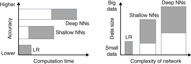
Figure 12.9 Qualitative assessment of neural networks.
12.4 Application: Image Recognition
12.4.1 Background
Statistical learning methods can be categorized into two broad areas: supervised learning and unsupervised learning. In the case of supervised learning, the “right answer” is given for a set of sample points. Techniques include predictive methods such as linear regression, logistic regression, and neural networks, as described in this book. It also includes classification methods such as binary classification where each sample is assigned to one of two possible groups, as is described shortly. On the other hand, in unsupervised learning, the “right answer” is not given so the techniques must discover relationships between the sample points. Well‐known methods in this category include ![]() ‐means clustering, anomaly detection, and dimensionality reduction (cf. James et al. 2013).
‐means clustering, anomaly detection, and dimensionality reduction (cf. James et al. 2013).
In this section, we describe an application of supervised learning for binary classification using logistic regression, shallow neural networks, and deep neural networks. We build regression‐based models using training data and then validate the accuracy using test data. The accuracy is determined by the number of correct predictions made on samples in the test set. The experimental setup is shown in Figure 12.10.

Figure 12.10 Typical setup for supervised learning methods.
The sequence of steps is as follows. First, the supervised training data ![]() is applied to the selected regression‐based model, either logistic regression, shallow NN or deep NN, in order to compute the
is applied to the selected regression‐based model, either logistic regression, shallow NN or deep NN, in order to compute the ![]() parameters. The accuracy of the model generated using the training data is usually quite high when measured on the same training data. Typically, it is 80–
parameters. The accuracy of the model generated using the training data is usually quite high when measured on the same training data. Typically, it is 80–![]() depending on the application. This can be misleading since the goal of the optimization is to closely match the training data and, in fact, a close match is produced. But that does not necessarily translate to the same accuracy on new data that is not in the training set. Therefore, it must also be evaluated on an independent set of test data
depending on the application. This can be misleading since the goal of the optimization is to closely match the training data and, in fact, a close match is produced. But that does not necessarily translate to the same accuracy on new data that is not in the training set. Therefore, it must also be evaluated on an independent set of test data ![]() to properly assess its accuracy. This is carried out by applying
to properly assess its accuracy. This is carried out by applying ![]() to the derived model and then comparing the predicted result
to the derived model and then comparing the predicted result ![]() against
against ![]() .
.
When given an initial data set, it is important to divide it into two sets, one for training and another for testing. For small data sets, ![]() is used for training and
is used for training and ![]() is used for testing. As a practical matter, there is usually a cross‐validation test set used during the development of the model to improve the model and then the final model evaluation is performed using the test set. Furthermore, on big data sets,
is used for testing. As a practical matter, there is usually a cross‐validation test set used during the development of the model to improve the model and then the final model evaluation is performed using the test set. Furthermore, on big data sets, ![]() may be used for training, while
may be used for training, while ![]() is used for cross‐validation and
is used for cross‐validation and ![]() for testing. Here we will consider only the training set and test set to simplify the presentation and use roughly
for testing. Here we will consider only the training set and test set to simplify the presentation and use roughly ![]() to train and
to train and ![]() to test the models.
to test the models.
12.4.2 Binary Classification
In order to compare the accuracy and speed of logistic regression, shallow neural networks and deep neural networks, a suitable application must be selected. One such application is binary classification of images, which is a simple form of image recognition. The problem of binary classification involves the task of deciding whether a set of images belongs to one group or another. The two groups are assigned the labels of 1 or 0. A label of 1 indicates that it belongs in the target group whereas a label of 0 signifies that it does not.
Specifically, if we are given a set of images of cats and dogs, we could label the cat pictures as 1 and the non‐cat pictures (i.e. pictures of dogs) as 0. Our training set has 100 images, with 50 cats and 50 dogs, and we label each one appropriately and use this to train a logistic regression model or a neural network. After training, we test the model on a set of 35 new images and evaluate the accuracy of the model. We also keep track of the amount of computer time to determine the trade‐off between accuracy and speed of the different methods.
Table 12.1 shows representative results from this type of analysis to set the context for experiments to be described in later sections. Column 1 indicates the test sample number, where we have listed only 10 samples of the test set. The next ![]() columns are the input values
columns are the input values ![]() ,
, ![]() ,
, ![]() ,
, ![]() associated with each image. Only the first few data values are shown here. The method used to convert images into these
associated with each image. Only the first few data values are shown here. The method used to convert images into these ![]() values is described in the next section. The next column in the table is
values is described in the next section. The next column in the table is ![]() , which is the correct label (0 or 1) for the image. And, finally,
, which is the correct label (0 or 1) for the image. And, finally, ![]() is the value predicted by the model, which will range between 0 and 1 since it is the output of a logistic function. This value is compared to 0.5 to quantize it to a label of either 0 or 1, which is also provided in the table.
is the value predicted by the model, which will range between 0 and 1 since it is the output of a logistic function. This value is compared to 0.5 to quantize it to a label of either 0 or 1, which is also provided in the table.
Table 12.1 Test data input, output, and predicted values from a binary classification model.
| 1 | 0.306 | 0.898 | 0.239 | — | 1 | 0.602 = 1 | tp |
| 2 | 0.294 | 0.863 | 0.176 | — | 1 | 0.507 = 1 | tp |
| 3 | 0.361 | 0.835 | 0.125 | — | 1 | 0.715 = 1 | tp |
| 4 | 0.310 | 0.902 | 0.235 | — | 0 | 0.222 = 0 | tn |
| 5 | 0.298 | 0.871 | 0.173 | — | 1 | 0.624 = 1 | tp |
| 6 | 0.365 | 0.863 | 0.122 | — | 1 | 0.369 = 0 | fp |
| 7 | 0.314 | 0.741 | 0.235 | — | 1 | 0.751 = 1 | tp |
| 8 | 0.302 | 0.733 | 0.173 | — | 0 | 0.343 = 0 | tn |
| 9 | 0.369 | 0.745 | 0.122 | — | 0 | 0.698 = 1 | fn |
| 10 | 0.318 | 0.757 | 0.239 | — | 0 | 0.343 = 0 | tn |
To assess the accuracy of each model, we could simply take the correct results and divide it by the total number of test samples to determine the success rate. However, this type of analysis, although useful as a first‐order assessment, may be misleading if most of the test data are cat pictures. Then by guessing 1 in all cases, a high accuracy can be obtained, but it would not be a true indication of the accuracy of the model. Instead, it is common practice to compute the ![]() score as follows. First, we categorize each sample based on whether or not the model predicted the correct label of 1 or 0. There are four possible scenarios, as listed in Table 12.2.
score as follows. First, we categorize each sample based on whether or not the model predicted the correct label of 1 or 0. There are four possible scenarios, as listed in Table 12.2.
Table 12.2 Interpretation of test set results.
| Interpretation | ||
| 1 | 1 | tp = true positive |
| 0 | 0 | tn = true negative |
| 1 | 0 | fp = false positive |
| 0 | 1 | fn = false negative |
For example, if the correct value is 1 and the quantized model predicts 1, it is referred to as a true positive (tp). Similarly a correct value of 0 and a predicted value of 0 is called a true negative (tn). On the other hand, incorrect predictions are either false positives (fp) or false negatives (fn). We can simply categorize each result and count up the numbers in each category. Then, using this information, we compute the recall and precision, which are both standard terms in binary classification (cf. James et al. 2013). Finally, the ![]() score is computed using these two quantities to assess the overall effectiveness of the model.
score is computed using these two quantities to assess the overall effectiveness of the model.
In particular, the recall value is given by

and the precision value is given by

Then, the ![]() score is computed using
score is computed using

For the example of Table 12.1 using only the 10 samples shown, the ![]() , the
, the ![]() , and the
, and the ![]() score
score ![]() . The optimal value of
. The optimal value of ![]() score is 1, so this would be a relatively good
score is 1, so this would be a relatively good ![]() score.
score.
12.4.3 Image Preparation
In order to carry out binary classification, images must be converted into values. The basic idea is to partition images into picture elements (pixels) and assign a number to each pixel based on the intensity and color of the image in that pixel. A set of images were prepared in this manner to train and test models for logistic regression, shallow neural networks, and deep neural networks. Each image was preprocessed as shown in Figure 12.11. First, the image was divided into pixels as illustrated in the figure. For simplicity, the case of ![]() pixels is shown here to produce a total of 16 pixels. However, there are three possible color combinations (RGB = red, green, blue) for each pixel resulting in a total of
pixels is shown here to produce a total of 16 pixels. However, there are three possible color combinations (RGB = red, green, blue) for each pixel resulting in a total of ![]() pixels in this example. Next, the values are “unrolled” to create one long
pixels in this example. Next, the values are “unrolled” to create one long ![]() vector. In the case to be presented in the experimental results shortly, images were actually divided into
vector. In the case to be presented in the experimental results shortly, images were actually divided into ![]() pixels to obtain higher resolution for image recognition purposes.
pixels to obtain higher resolution for image recognition purposes.

Figure 12.11 Preparing the image for model building.
Each image was assigned the proper observed ![]() value of
value of ![]() or
or ![]() . A total of 100 images were used to build models, and 35 images were used to test the model. Each model was generated first without a penalty function and then with the ridge and LASSO penalty functions. To illustrate the expected effect of ridge or LASSO penalty on the data, a simple case of two independent variables is shown in Figure 12.12. In the actual case, there are
. A total of 100 images were used to build models, and 35 images were used to test the model. Each model was generated first without a penalty function and then with the ridge and LASSO penalty functions. To illustrate the expected effect of ridge or LASSO penalty on the data, a simple case of two independent variables is shown in Figure 12.12. In the actual case, there are ![]() independent variables as mentioned, but two variables are sufficient to describe conceptually the effect of a penalty function in binary classification.
independent variables as mentioned, but two variables are sufficient to describe conceptually the effect of a penalty function in binary classification.
In the figure, the 1's represent cats, while 0's represent dogs. The model defines the decision boundary between the two classes. In Figure 12.12a, neither ridge nor LASSO is used so the decision boundary is some complex path through the data. This over‐fitted situation produces ![]() accuracy on the training data. With the
accuracy on the training data. With the ![]() or
or ![]() penalty applied, a smoother curve is expected, as in Figure 12.12b for
penalty applied, a smoother curve is expected, as in Figure 12.12b for ![]() . In this case, the training data accuracy is below
. In this case, the training data accuracy is below ![]() because some cats have been misclassified as dogs and vice versa. On the other hand, it will likely be more accurate on test data since the decision boundary is more realistic. The inherent errors are due to the fact that some cat images may appear to look like dogs, while dog pictures may appear to look like cats. But, in general, the smoother curve is preferred as opposed to the over‐fitted result. In fact, this is why the ridge penalty function is widely used in neural networks.
because some cats have been misclassified as dogs and vice versa. On the other hand, it will likely be more accurate on test data since the decision boundary is more realistic. The inherent errors are due to the fact that some cat images may appear to look like dogs, while dog pictures may appear to look like cats. But, in general, the smoother curve is preferred as opposed to the over‐fitted result. In fact, this is why the ridge penalty function is widely used in neural networks.

Figure 12.12 Over‐fitting vs. regularized training data. (a) Over‐fitting. (b) Effect of  penalty.
12.4.4 Experimental Results
A set of ![]() images of cats and dogs (50 each) were used as training data for a series of regression models. An additional 35 images were used as test data. As mentioned, for each sample image, there are
images of cats and dogs (50 each) were used as training data for a series of regression models. An additional 35 images were used as test data. As mentioned, for each sample image, there are ![]() independent variables (the “unrolled” pixels) and one dependent variable (
independent variables (the “unrolled” pixels) and one dependent variable (![]() cat,
cat, ![]() dog). Clearly, this is a very wide data set where over‐fitting would be a significant problem. Therefore, some type of penalty function is needed in conjunction with the loss function, as described in earlier sections. Numerical methods were used to determine the
dog). Clearly, this is a very wide data set where over‐fitting would be a significant problem. Therefore, some type of penalty function is needed in conjunction with the loss function, as described in earlier sections. Numerical methods were used to determine the ![]() parameters for each regression model by minimizing the loss function using gradient descent, with a step size of
parameters for each regression model by minimizing the loss function using gradient descent, with a step size of ![]() . The solution space was assumed to be convex and so a simple gradient descent was sufficient to minimize the loss value and obtain the corresponding
. The solution space was assumed to be convex and so a simple gradient descent was sufficient to minimize the loss value and obtain the corresponding ![]() values. The number of iterations of gradient descent was initially set to 3000. In the first run of each model, the tuning parameter
values. The number of iterations of gradient descent was initially set to 3000. In the first run of each model, the tuning parameter ![]() was set to 0 (i.e. no penalty function). Then it was varied between 0.1 and 10.0 for both
was set to 0 (i.e. no penalty function). Then it was varied between 0.1 and 10.0 for both ![]() ‐penalty and
‐penalty and ![]() ‐penalty functions. The results are shown in Tables 12.3–12.6.
‐penalty functions. The results are shown in Tables 12.3–12.6.
Table 12.3 contains the results for logistic regression (LR) using the ![]() ‐penalty function; as
‐penalty function; as ![]() is increased from 0.0 to 10.0, the effect of the penalty function increases. This can be understood by examining the columns labeled test accuracy and
is increased from 0.0 to 10.0, the effect of the penalty function increases. This can be understood by examining the columns labeled test accuracy and ![]() score. Initially, the test accuracy increases as
score. Initially, the test accuracy increases as ![]() is increased until an optimal value of the test accuracy is achieved. The optimal result is obtained for
is increased until an optimal value of the test accuracy is achieved. The optimal result is obtained for ![]() and this case delivers a test accuracy of
and this case delivers a test accuracy of ![]() along with the highest
along with the highest ![]() score of 0.77. This implies that
score of 0.77. This implies that ![]() of the 35 test images were correctly identified as a cat or dog, after training on the 100 sample images with
of the 35 test images were correctly identified as a cat or dog, after training on the 100 sample images with ![]() accuracy. However, increasing the value of
accuracy. However, increasing the value of ![]() further does not improve the test accuracy and, in fact, it begins to degrade at very high values.
further does not improve the test accuracy and, in fact, it begins to degrade at very high values.
Table 12.3 Results for ![]() ‐penalty (ridge) using LR.
‐penalty (ridge) using LR.
| Train accuracy (%) | Testing accuracy (%) | Runtime (s) | ||
| 100 | 68.6 | 0.72 | 14.9 | |
| 100 | 68.6 | 0.72 | 15.2 | |
| 100 | 74.3 | 16.6 | ||
| 100 | 71.4 | 0.74 | 15.3 | |
| 100 | 71.4 | 0.74 | 12.5 | |
| 100 | 68.6 | 0.72 | 15.7 | |
| 100 | 60.0 | 0.63 | 15.4 |
Table 12.4 Results for ![]() ‐penalty (LASSO) using LR.
‐penalty (LASSO) using LR.
| Train accuracy (%) | Testing accuracy (%) | Runtime (s) | ||
| 100 | 68.6 | 0.72 | 14.8 | |
| 100 | 71.4 | 14.9 | ||
| 100 | 62.9 | 0.70 | 15.3 | |
| 100 | 60.0 | 0.65 | 15.3 | |
| 97 | 60.0 | 0.65 | 15.4 | |
| 57 | 57.1 | 0.61 | 15.7 |
Table 12.4 indicates that the ![]() penalty has difficulty in improving the results beyond those obtained from the
penalty has difficulty in improving the results beyond those obtained from the ![]() penalty. Inherently, LASSO seeks to zero out some of the parameters, but since the inputs are all pixels of images, no variables can be eliminated. Another effect is due to slow convergence of gradient descent when the
penalty. Inherently, LASSO seeks to zero out some of the parameters, but since the inputs are all pixels of images, no variables can be eliminated. Another effect is due to slow convergence of gradient descent when the ![]() ‐penalty is used. One can increase the number of iterations beyond 3000 in this particular case, but it becomes computationally more expensive without delivering improvements over ridge. For these and other reasons, the
‐penalty is used. One can increase the number of iterations beyond 3000 in this particular case, but it becomes computationally more expensive without delivering improvements over ridge. For these and other reasons, the ![]() ‐penalty function is widely used in applications with characteristics similar to image recognition rather than the
‐penalty function is widely used in applications with characteristics similar to image recognition rather than the ![]() ‐penalty function.
‐penalty function.
The next model was built using a two‐layer neural network with one hidden layer with five units using only the ![]() ‐penalty function, since the
‐penalty function, since the ![]() ‐penalty function produced very poor results. The five hidden units used the
‐penalty function produced very poor results. The five hidden units used the ![]() function of Figure 12.8, while the output layer used the logistic function
function of Figure 12.8, while the output layer used the logistic function ![]() of Figure 12.3. The results are given in Table 12.5. To obtain the desired accuracy,
of Figure 12.3. The results are given in Table 12.5. To obtain the desired accuracy, ![]() iterations were required. Note that the accuracy of the model has improved greatly relative to logistic regression but the runtime has also increased. This is expected based on Figure 12.9 shown previously. In this case, each iteration requires operations on a
iterations were required. Note that the accuracy of the model has improved greatly relative to logistic regression but the runtime has also increased. This is expected based on Figure 12.9 shown previously. In this case, each iteration requires operations on a ![]() matrix so the runtime is much higher. However, the test accuracy is now
matrix so the runtime is much higher. However, the test accuracy is now ![]() with a corresponding
with a corresponding ![]() score of 0.84.
score of 0.84.
Table 12.5 Results for ![]() ‐penalty (ridge) using two‐layer NN.
‐penalty (ridge) using two‐layer NN.
| Train accuracy (%) | Testing accuracy (%) | Runtime (s) | ||
| 100 | 77 | 0.79 | 184 | |
| 100 | 77 | 0.79 | 186 | |
| 100 | 77 | 0.79 | 187 | |
| 100 | 80 | 0.82 | 186 | |
| 100 | 82 | 192 | ||
| 100 | 77 | 0.79 | 202 | |
| 65 | 0.68 | 194 |
The final set of results are shown in Table 12.6 for a three‐layer neural network. There are two hidden layers with ten and five hidden units, respectively. All 15 hidden units used the ![]() function and, as before, the output function employed the logistic function
function and, as before, the output function employed the logistic function ![]() . While not strictly a deep neural network, it provides enough information to assess the accuracy and speed characteristics of deep networks. The best test accuracy of the different cases is
. While not strictly a deep neural network, it provides enough information to assess the accuracy and speed characteristics of deep networks. The best test accuracy of the different cases is ![]() with an
with an ![]() score of 0.82, which is lower than the two‐layer case, but the overall accuracy of all cases is higher. However, it is clearly more computationally expensive than the other models. This is due to the fact that it now operates on a
score of 0.82, which is lower than the two‐layer case, but the overall accuracy of all cases is higher. However, it is clearly more computationally expensive than the other models. This is due to the fact that it now operates on a ![]() matrix on each iteration of gradient descent. Therefore, it requires a higher runtime. In this case, a total of
matrix on each iteration of gradient descent. Therefore, it requires a higher runtime. In this case, a total of ![]() iterations were used to obtain the results.
iterations were used to obtain the results.
Table 12.6 Results for ![]() ‐penalty (ridge) using three‐layer NN.
‐penalty (ridge) using three‐layer NN.
| Train accuracy (%) | Testing accuracy (%) | Runtime (s) | ||
| 100 | 77 | 0.79 | 384 | |
| 100 | 80 | 0.82 optimal | 386 | |
| 100 | 80 | 0.82 | 387 | |
| 100 | 77 | 0.79 | 386 | |
| 100 | 77 | 0.79 | 392 | |
| 100 | 77 | 0.79 | 402 |
To summarize, the ![]() ‐penalty function is more effective on logistic and neural networks than the
‐penalty function is more effective on logistic and neural networks than the ![]() ‐penalty function for image recognition. These penalty functions are best suited to wide data sets where over‐fitting is the main problem. It is very useful in shallow neural networks, but less effective as more layers are used in the network. One should note that the results are controlled to a large extent by a set of tunable hyper‐parameters:
‐penalty function for image recognition. These penalty functions are best suited to wide data sets where over‐fitting is the main problem. It is very useful in shallow neural networks, but less effective as more layers are used in the network. One should note that the results are controlled to a large extent by a set of tunable hyper‐parameters: ![]() ,
, ![]() the number of layers, the number of hidden units in each layer, and the number of iterations used to build the model. Furthermore, additional improvements can be obtained by increasing the size of the sample set. An important part of using neural networks is to properly determine these (and other) tunable hyper‐parameters to deliver optimal results. In any case, it is clear that the ridge penalty function is a critical part of neural networks and worth pursuing as future research.
the number of layers, the number of hidden units in each layer, and the number of iterations used to build the model. Furthermore, additional improvements can be obtained by increasing the size of the sample set. An important part of using neural networks is to properly determine these (and other) tunable hyper‐parameters to deliver optimal results. In any case, it is clear that the ridge penalty function is a critical part of neural networks and worth pursuing as future research.
12.5 Summary and Concluding Remarks
In this chapter, we used logistic regression in neural networks, from the importance of penalty functions. As we outlines in Section 12.1, we dealt with the practical application of penalty functions and their use in applied statistics. In conclusion, we found the ![]() ‐penalty function is more effective on logistic and neural networks than the
‐penalty function is more effective on logistic and neural networks than the ![]() ‐penalty function.
‐penalty function.
Problems
- 12.1
Derive the updated equations for
 and
and  for a two‐layer neural network that is similar in form to (12.19) assuming the logistic function is used in both layers.
 - 12.2
Another possible activation function (that is, a function that would play the role of the logistic function) is the
 function. Derive the updated equations for a two‐layer neural network if the
  function is used in the first layer and the logistic function is used in the second layer.
 - 12.3
Derive the gradient equation for the
 activation function where

- 12.4 The figure depicts a four‐layer neural network. Based on Figure 12.6, what are the sizes of the respective
 matrices or vector for each stage? (Hint: the matrix for layer 1 is
  since the first layer has five hidden units and the input has four variables).

- 12.5 Derive equations similar to (12.20) for the deep neural network shown. You can assume that the logistic function is used in every layer.