6
Ridge Regression in Theory and Applications
The multiple linear regression model is one of the best known and widely used among the models for statistical data analysis in every field of sciences and engineering as well as in social sciences, economics, and finance. The subject of this chapter is the study of the rigid regression estimator (RRE) for the regression coefficients, its characteristic properties, and comparing its relation with the least absolute shrinkage and selection operator (LASSO). Further, we consider the preliminary test estimator (PTE) and the Stein‐type ridge estimator in low dimension and study their dominance properties. We conclude the chapter with the asymptotic distributional theory of the ridge estimators following Knight and Fu (2000).
6.1 Multiple Linear Model Specification
Consider the multiple linear model with coefficient vector, ![]() given by
given by
where ![]() is a vector of
is a vector of ![]() responses,
responses, ![]() is an
is an ![]() design matrix of rank
design matrix of rank ![]() , and
, and ![]() is an
is an ![]() ‐vector of independently and identically distributed (i.i.d.) random variables with distribution
‐vector of independently and identically distributed (i.i.d.) random variables with distribution ![]() , with
, with ![]() , the identity matrix of order
, the identity matrix of order ![]() .
.
6.1.1 Estimation of Regression Parameters
Using the model (6.1) and the error distribution of ![]() we obtain the maximum likelihood estimator/least squares estimator (MSE/LSE) of
we obtain the maximum likelihood estimator/least squares estimator (MSE/LSE) of ![]() by minimizing
by minimizing
to get ![]() , where
, where ![]() ,
, ![]() .
.
Sometimes the method is written as
where ![]() , and
, and ![]() where
where ![]() and
and ![]() are
are ![]() and
and ![]() submatrices, respectively,
submatrices, respectively, ![]() of dimension
of dimension ![]() stands for the main effect, and
stands for the main effect, and ![]() of dimension
of dimension ![]() stands for the interactions; and we like estimate
stands for the interactions; and we like estimate ![]() . Here,
. Here, ![]() .
.
In this case, we may write

where ![]() ,
, ![]() . Hence
. Hence

where

respectively.
It is well known that ![]() and the covariance matrix of
and the covariance matrix of ![]() is given by
is given by

Further, an unbiased estimator of ![]() is given by
is given by
Using normal theory it may be shown that ![]() are statistically independent and
are statistically independent and ![]() and
and ![]() follows a central chi‐square distribution with
follows a central chi‐square distribution with ![]() degrees of freedom (DF).
degrees of freedom (DF).
The ![]() risk of
risk of ![]() , any estimator of
, any estimator of ![]() , is defined by
, is defined by
Then, the ![]() risk of
risk of ![]() is given by
is given by
If ![]() be the eigenvalues of
be the eigenvalues of ![]() , then we may write
, then we may write

Similarly, one notes that

In a similar manner, ![]() .
.
Now, we find the ![]() and
and ![]() as given below
as given below

Similarly, we obtain
6.1.2 Test of Hypothesis for the Coefficients Vector
Suppose we want to test the null‐hypothesis ![]() vs.
vs. ![]() . Then, we use the test statistic (likelihood ratio test),
. Then, we use the test statistic (likelihood ratio test),

which follows a noncentral ![]() ‐distribution with
‐distribution with ![]() DF and noncentrality parameter,
DF and noncentrality parameter, ![]() , defined by
, defined by

Similarly, if we want to test the subhypothesis ![]() vs.
vs. ![]() , then one may use the test statistic
, then one may use the test statistic

where ![]() ,
, ![]() and
and

Note that ![]() follows a noncentral
follows a noncentral ![]() ‐distribution with
‐distribution with ![]() DF and noncentrality parameter
DF and noncentrality parameter ![]() given by
given by

Let ![]() be the upper
be the upper ![]() ‐level critical value for the test of
‐level critical value for the test of ![]() , then we reject
, then we reject ![]() whenever
whenever ![]() or
or ![]() ; otherwise, we accept
; otherwise, we accept ![]() .
.
6.2 Ridge Regression Estimators (RREs)
From Section 6.1.1, we may see that

- cov‐matrix of
 is
is  .
.
Hence, ![]() ‐risk function of
‐risk function of ![]() is
is ![]() . Further, when
. Further, when ![]() , the variance of
, the variance of ![]() is
is ![]() .
.
Set ![]() . Then, it is seen that the lower bound of the
. Then, it is seen that the lower bound of the ![]() risk and the variance are
risk and the variance are ![]() and
and ![]() , respectively. Hence, the shape of the parameter space is such that reasonable data collection may result in a
, respectively. Hence, the shape of the parameter space is such that reasonable data collection may result in a ![]() matrix with one or more small eigenvalues. As a result,
matrix with one or more small eigenvalues. As a result, ![]() distance of
distance of ![]() to
to ![]() will tend to be large. In particular, coefficients tend to become large in absolute value and may even have wrong signs and be unstable. As a result, such difficulties increase as more prediction vectors deviate from orthogonality. As the design matrix,
will tend to be large. In particular, coefficients tend to become large in absolute value and may even have wrong signs and be unstable. As a result, such difficulties increase as more prediction vectors deviate from orthogonality. As the design matrix, ![]() deviates from orthogonality,
deviates from orthogonality, ![]() becomes smaller and
becomes smaller and ![]() will be farther away from
will be farther away from ![]() . The ridge regression method is a remedy to circumvent these problems with the LSE.
. The ridge regression method is a remedy to circumvent these problems with the LSE.
For the model (6.1), Hoerl and Kennard (1970) defined the RRE of ![]() as
as
The basic idea of this type is from Tikhonov (1963) where the tuning parameter, ![]() , is to be determined from the data
, is to be determined from the data ![]() . The expression (6.17) may be written as
. The expression (6.17) may be written as
If ![]() is invertible, whereas if
is invertible, whereas if ![]() is ill‐conditioned or near singular, then (6.17) is the appropriate expression for the estimator of
is ill‐conditioned or near singular, then (6.17) is the appropriate expression for the estimator of ![]() .
.
The derivation of (6.17) is very simple. Instead of minimizing the LSE objective function, one may minimize the objective function where ![]() is the penalty function
is the penalty function
with respect to (w.r.t.) ![]() yielding the normal equations,
yielding the normal equations,
Here, we have equal weight to the components of ![]() .
.
6.3 Bias, MSE, and  Risk of Ridge Regression Estimator
In this section, we consider bias, mean squared error (MSE), and ![]() ‐risk expressions of the RRE.
‐risk expressions of the RRE.
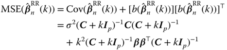
First, we consider the equal weight RRE, ![]() . The bias, MSE, and
. The bias, MSE, and ![]() risk are obtained as
risk are obtained as

respectively.
One may write

Let ![]() and
and ![]() be the
be the ![]() th eigenvalue of
th eigenvalue of ![]() and
and ![]() , respectively. Then
, respectively. Then

![]() .
.
Note that
 , for
, for  , is shorter than
  , that is
(6.26)
, that is
(6.26)
- (6.27)where

 .
.
For the estimate of ![]() , the residual sum of squares (RSS) is
, the residual sum of squares (RSS) is

The expression shows that the RSS in (6.28) is equal to the total sum of squares due to ![]() with a modification upon the squared length of
with a modification upon the squared length of ![]() .
.
Now, we explain the properties of ![]() risk of the RSS given in (6.28), which may be written as
risk of the RSS given in (6.28), which may be written as

Figure 6.1, the graph of the ![]() risk, depicts the two components as a function of
risk, depicts the two components as a function of ![]() . It shows the relationships between variances, the quadratic bias and
. It shows the relationships between variances, the quadratic bias and ![]() , the tuning parameter.
, the tuning parameter.

Figure 6.1 Graph of  risk of RRE in case of
  .
.
Total variance decreases as ![]() increases, while quadratic bias increases with
increases, while quadratic bias increases with ![]() . As indicated by the dotted line graph representing RRE
. As indicated by the dotted line graph representing RRE ![]() risk, there are values of
risk, there are values of ![]() for which
for which ![]() is less than or equal to
is less than or equal to ![]() .
.
It may be noted that ![]() is a monotonic decreasing function of
is a monotonic decreasing function of ![]() , which
, which ![]() is a monotonic increasing function of
is a monotonic increasing function of ![]() . Now, find the derivatives of these two functions at the origin (
. Now, find the derivatives of these two functions at the origin (![]() ) as
) as

Hence, ![]() has a negative derivative, which tends to
has a negative derivative, which tends to ![]() as
as ![]() for an orthogonal
for an orthogonal ![]() and approaches
and approaches ![]() as
as ![]() becomes ill‐conditioned and
becomes ill‐conditioned and ![]() , while as
, while as ![]() ,
, ![]() is flat and zero at
is flat and zero at ![]() . These properties indicate that if we choose
. These properties indicate that if we choose ![]() appropriately, our estimator will inherit a little bias and substantially reduce variances, and thereby the
appropriately, our estimator will inherit a little bias and substantially reduce variances, and thereby the ![]() ‐risk will decrease to improve the prediction.
‐risk will decrease to improve the prediction.
We now prove the existence of ![]() to validate the commentaries put forward by the following theorems.
to validate the commentaries put forward by the following theorems.
A direct consequence of the given result is the following existence theorem.
6.4 Determination of the Tuning Parameters
Suppose ![]() is nonsingular, then the LSE of
is nonsingular, then the LSE of ![]() is
is ![]() . Let
. Let ![]() be the equal weight RRE of
be the equal weight RRE of ![]() deleting the
deleting the ![]() th data point
th data point ![]() . If
. If ![]() is chosen properly, then the
is chosen properly, then the ![]() th component of
th component of ![]() predicts
predicts ![]() well. The generalized cross‐validation (GCV) is defined as the weight average of predicted square errors
well. The generalized cross‐validation (GCV) is defined as the weight average of predicted square errors

where ![]() and
and ![]() is the
is the ![]() th diagonal element of
th diagonal element of ![]() . See Golub et al. (1979) for more details.
. See Golub et al. (1979) for more details.
A computationally efficient version of the GCV function of the RRE is

The GCV estimator of ![]() is then given by
is then given by
The GCV theorem (Golub et al. 1979) guarantees the asymptotic efficiency of the GCV estimator under ![]() (and also
(and also ![]() ) setups.
) setups.
We later see that the statistical estimator of ![]() is given by
is given by ![]() , where
, where ![]() .
.
6.5 Ridge Trace
Ridge regression has two interpretations of its characteristics. The first is the ridge trace. It is a two‐dimensional plot of ![]() and the RSS given by
and the RSS given by
for a number of values of ![]() . The trace serves to depict the complex relationships that exist between nonorthogonal prediction vectors and the effect of these interrelationships on the estimation of
. The trace serves to depict the complex relationships that exist between nonorthogonal prediction vectors and the effect of these interrelationships on the estimation of ![]() . The second is the way to estimate
. The second is the way to estimate ![]() that gives a better estimator of
that gives a better estimator of ![]() by damping the effect of the lower bound mentioned earlier. Ridge trace is a diagnostic test that gives a readily interpretable picture of the effects of nonorthogonality and may guide to a better point estimate.
by damping the effect of the lower bound mentioned earlier. Ridge trace is a diagnostic test that gives a readily interpretable picture of the effects of nonorthogonality and may guide to a better point estimate.
Now, we discuss how ridge regression can be used by statisticians with the gasoline mileage data from Montgomery et al. (2012). The data contains the following variables: ![]() = miles/gallon,
= miles/gallon, ![]() = displacement (cubic in.),
= displacement (cubic in.), ![]() = horsepower (ft‐lb),
= horsepower (ft‐lb), ![]() = torque (ft‐lb),
= torque (ft‐lb), ![]() = compression ratio,
= compression ratio, ![]() = rear axle ratio,
= rear axle ratio, ![]() = carburetor (barrels),
= carburetor (barrels), ![]() = number of transmission speeds,
= number of transmission speeds, ![]() = overall length,
= overall length, ![]() =
= ![]() = width (in.),
= width (in.), ![]() = weight (lb),
= weight (lb), ![]() = type of transmission.
= type of transmission.
Table 6.1 is in correlation format of ![]() and
and ![]() , where
, where ![]() is centered.
is centered.
Table 6.1 Correlation coefficients for gasoline mileage data.
| 1.0 | 0.4 | 0.6 | 0.7 | |||||||||
| 1.0 | 0.9 | 0.9 | 0.6 | 0.8 | 0.7 | 0.9 | 0.8 | |||||
| 0.9 | 1.0 | 0.9 | 0.7 | 0.8 | 0.7 | 0.8 | 0.7 | |||||
| 0.9 | 0.9 | 1.0 | 0.6 | 0.8 | 0.7 | 0.9 | 0.8 | |||||
| 0.4 | 1.0 | 0.4 | 0.0 | 0.5 | ||||||||
| 0.6 | 0.4 | 1.0 | 0.8 | |||||||||
| 0.6 | 0.7 | 0.6 | 0.0 | 1.0 | 0.4 | 0.3 | 0.5 | 0.3 | ||||
| 0.7 | 0.5 | 0.8 | 1.0 | |||||||||
| 0.8 | 0.8 | 0.8 | 0.4 | 1.0 | 0.8 | 0.9 | 0.6 | |||||
| 0.7 | 0.7 | 0.7 | 0.3 | 0.8 | 1.0 | 0.8 | 0.6 | |||||
| 0.9 | 0.8 | 0.9 | 0.5 | 0.9 | 0.8 | 1.0 | 0.7 | |||||
| 0.8 | 0.7 | 0.8 | 0.3 | 0.6 | 0.6 | 0.7 | 1.0 |
We may find that the eigenvalues of the matrix ![]() are given by
are given by ![]() ,
, ![]() ,
, ![]() ,
, ![]() ,
, ![]() ,
, ![]() ,
, ![]() ,
, ![]() ,
, ![]() ,
, ![]() , and
, and ![]() .
.
The condition number is ![]() , which indicates serious multicollinearity. They are nonzero real numbers and
, which indicates serious multicollinearity. They are nonzero real numbers and ![]() , which is 1.6 times more than 10 in the orthogonal case. Thus, it shows that the expected distance of the BLUE (best linear unbiased estimator),
, which is 1.6 times more than 10 in the orthogonal case. Thus, it shows that the expected distance of the BLUE (best linear unbiased estimator), ![]() from
from ![]() is
is ![]() . Thus, the parameter space of
. Thus, the parameter space of ![]() is
is ![]() ‐dimensional, but most of the variations are due to the largest two eigenvalues.
‐dimensional, but most of the variations are due to the largest two eigenvalues.
Variance inflation factor (VIF): First, we want to find VIF, which is defined as

where ![]() is the coefficient of determination obtained when
is the coefficient of determination obtained when ![]() is regressed on the remaining
is regressed on the remaining ![]() regressors. A
regressors. A ![]() greater than 5 or 10 indicates that the associated regression coefficients are poor estimates because of multicollinearity.
greater than 5 or 10 indicates that the associated regression coefficients are poor estimates because of multicollinearity.
The VIF of the variables in this data set are as follows: ![]() ,
, ![]() ,
, ![]() ,
, ![]() ,
, ![]() ,
, ![]() ,
, ![]() ,
, ![]() ,
, ![]() ,
, ![]() , and
, and ![]() . These VIFs certainly indicate severe multicollinearity in the data. It is also evident from the correlation matrix in Table 6.1. This is the most appropriate data set to analyze ridge regression.
. These VIFs certainly indicate severe multicollinearity in the data. It is also evident from the correlation matrix in Table 6.1. This is the most appropriate data set to analyze ridge regression.
On the other hand, one may look at the ridge trace and discover many finer details of each factor and the optimal value of ![]() , the tuning parameter of the ridge regression errors. The ridge trace gives a two‐dimensional portrayal of the effect of factor correlations and making possible assessments that cannot be made even if all regressions are computed. Figure 6.2 depicts the analysis using the ridge trace.
, the tuning parameter of the ridge regression errors. The ridge trace gives a two‐dimensional portrayal of the effect of factor correlations and making possible assessments that cannot be made even if all regressions are computed. Figure 6.2 depicts the analysis using the ridge trace.

Figure 6.2 Ridge trace for gasoline mileage data.
Notice that the absolute value of each factor tends to the LSE as ![]() goes to zero. From Figure 6.2 we can see that reasonable coefficient stability is achieved in the range
goes to zero. From Figure 6.2 we can see that reasonable coefficient stability is achieved in the range ![]() . For more comments, see Hoerl and Kennard (1970).
. For more comments, see Hoerl and Kennard (1970).
6.6 Degrees of Freedom of RRE
RRE constraints the flexibility of the model by adding a quadratic penalty term to the least squares objective function (see Section 6.2).
When ![]() , the RRE equals the LSE. The larger the value of
, the RRE equals the LSE. The larger the value of ![]() , the greater the penalty for having large coefficients.
, the greater the penalty for having large coefficients.
In our study, we use ![]() ‐risk expression to assess the overall quality of an estimator. From (6.7) we see that the
‐risk expression to assess the overall quality of an estimator. From (6.7) we see that the ![]() risk of the LSE,
risk of the LSE, ![]() is
is ![]() and from (6.23) we find the
and from (6.23) we find the ![]() risk of RRE is
risk of RRE is
These expressions give us the distance of LSE and RRE from the true value of ![]() , respectively. LSE is a BLUE of
, respectively. LSE is a BLUE of ![]() . But RRE is a biased estimator of
. But RRE is a biased estimator of ![]() . It modifies the LSE by introducing a little bias to improve its performance. The RRE existence in Theorem 6.2 shows that for
. It modifies the LSE by introducing a little bias to improve its performance. The RRE existence in Theorem 6.2 shows that for ![]() ,
, ![]() . Thus, for an appropriate choice of
. Thus, for an appropriate choice of ![]() , RRE is closer to
, RRE is closer to ![]() than to the LSE. In this sense, RRE is more reliable than the LSE.
than to the LSE. In this sense, RRE is more reliable than the LSE.
On top of the abovementioned property, RRE improves the model performance over the LSE and variable subset selection. RRE also reduces the model DF For example, LSE has ![]() parameters and therefore uses
parameters and therefore uses ![]() DF.
DF.
To see how RRE reduces the number of parameters, we define linear smoother given by
where the linear operator ![]() is a smoother matrix and
is a smoother matrix and ![]() contains the predicted value of
contains the predicted value of ![]() . The DF of
. The DF of ![]() is given by the trace of the smoother matrix,
is given by the trace of the smoother matrix, ![]() . The LSE and RRE are both linear smoother, since the predicted values of either estimators are given by the product
. The LSE and RRE are both linear smoother, since the predicted values of either estimators are given by the product
where ![]() is the hat matrix of the RRE. Let
is the hat matrix of the RRE. Let ![]() be the hat matrix of the LSE, then
be the hat matrix of the LSE, then ![]() is the DF of LSE.
is the DF of LSE.
To find the DF of RRE, let ![]() ,
, ![]() ,
, ![]() be the eigenvalue matrix corresponding to
be the eigenvalue matrix corresponding to ![]() . We consider the singular value decomposition (SVD) of
. We consider the singular value decomposition (SVD) of ![]() , where
, where ![]() and
and ![]() are column orthogonal matrices; then
are column orthogonal matrices; then

where ![]() are called the shrinkage fractions. When
are called the shrinkage fractions. When ![]() is positive, the shrinkage fractions are all less than 1 and, hence,
is positive, the shrinkage fractions are all less than 1 and, hence, ![]() . Thus, the effective number of parameters in a ridge regression model is less than the actual number of predictors. The variable subset selection method explicitly drops the variables from the model, while RRE reduces the effects of the unwanted variables without dropping them.
. Thus, the effective number of parameters in a ridge regression model is less than the actual number of predictors. The variable subset selection method explicitly drops the variables from the model, while RRE reduces the effects of the unwanted variables without dropping them.
A simple way of finding a value of ![]() is to set the equation
is to set the equation ![]() and solve for
and solve for ![]() . It is easy to see that
. It is easy to see that

Then, solve ![]() . Hence, an optimum value of
. Hence, an optimum value of ![]() falls in the interval
falls in the interval

such that ![]() .
.
6.7 Generalized Ridge Regression Estimators
In Sections 6.2 and 6.3, we discussed ordinary RREs and the associated bias and ![]() ‐risk properties. In this RRE, all coefficients are equally weighted; but in reality, the coefficients deserve unequal weight. To achieve this goal, we define the generalized ridge regression estimator (GRRE) of
‐risk properties. In this RRE, all coefficients are equally weighted; but in reality, the coefficients deserve unequal weight. To achieve this goal, we define the generalized ridge regression estimator (GRRE) of ![]() as
as
where ![]() ,
, ![]() ,
, ![]() . If
. If ![]() , we get (6.17). One may derive (6.38) by minimizing the objective function with
, we get (6.17). One may derive (6.38) by minimizing the objective function with ![]() as the penalty function
as the penalty function
w.r.t. ![]() to obtain the normal equations
to obtain the normal equations
Here, we have put unequal weight on the components of ![]() .
.
The bias, MSE, and ![]() ‐risk expressions of the GRRE given by
‐risk expressions of the GRRE given by


respectively.
In the next section, we show the application of the GRRE to obtain the adaptive RRE.
6.8 LASSO and Adaptive Ridge Regression Estimators
If the ![]() norm in the penalty function of the LSE objective function
norm in the penalty function of the LSE objective function
is replaced by the ![]() norm
norm ![]() , the resultant estimator is
, the resultant estimator is
This estimator makes some coefficients zero, making the LASSO estimator different from RRE where most of coefficients become small but nonzero. Thus, LASSO simultaneously selects and estimates at the same time.
The LASSO estimator may be written explicitly as
where ![]() is the
is the ![]() th diagonal element of
th diagonal element of ![]() and
and ![]() .
.
Now, if we consider the estimation of ![]() in the GRRE, it may be easy to see that if
in the GRRE, it may be easy to see that if ![]() ,
, ![]() ,
, ![]() , where
, where ![]() is an orthogonal matrix; see Hoerl and Kennard (1970).
is an orthogonal matrix; see Hoerl and Kennard (1970).
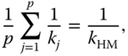
To avoid simultaneous estimation of the weights ![]() , we assume that
, we assume that ![]() in (6.47) is equal to the harmonic mean of
in (6.47) is equal to the harmonic mean of ![]() , i.e.
, i.e.

The value of ![]() controls the global complexity. This constraint is the link between the
controls the global complexity. This constraint is the link between the ![]() tuning parameters of
tuning parameters of ![]() and tuning parameter
and tuning parameter ![]() of
of ![]() .
.
The adaptive generalized ridge regression estimator (AGRRE) is obtained by minimizing the following objective function:
which is the Lagrangian form of the objective function
and ![]() and
and ![]() are the Lagrangian for (6.50).
are the Lagrangian for (6.50).
Following Avalos et al. (2007), a necessary condition for the optimality is obtained by deriving the Lagrangian w.r.t. ![]() , given by
, given by

Putting the expression in the constraint (6.49), we obtain

The optimal ![]() is then obtained from
is then obtained from ![]() and
and ![]() 's so that (6.51) may be written as
's so that (6.51) may be written as

which is equivalent to minimizing
for some ![]() , which is exactly LASSO problem.
, which is exactly LASSO problem.
Minimizing (6.55), we obtain ![]() normal equations for
normal equations for ![]() , as
, as

The solution (6.56) may be obtained following Grandvalet (1998) as given here:Let

Then, the problem (6.51) with constraint (6.52) may be written as
where ![]() with
with ![]() , subject to
, subject to ![]() ,
, ![]() ,
, ![]() .
.
After some tedious algebra, as in Avalos et al. (2007), we obtain the RRE of ![]() as
as

In the next section, we present the algorithm to obtain LASSO solutions.
6.9 Optimization Algorithm
For the computation of LASSO estimators, Tibshirani (1996) used quadratic programming. In this section, we use a fixed point algorithm from the expression (6.51) which is the GRRE. Thus, we solve a sequence of weighted ridge regression problems, as suggested by Knight and Fu (2000). First, we estimate ![]() ‐matrix based on the estimators of
‐matrix based on the estimators of ![]() as well as
as well as ![]() . For the estimator of
. For the estimator of ![]() , we use from Hoerl et al. (1975):
, we use from Hoerl et al. (1975):

where

Hence, the estimate of the diagonal matrix ![]() is given by
is given by ![]() , where
, where

Alternatively, we may use the estimator, ![]() , where
, where

The derivation of this estimator is explained here.
We consider the LASSO problem, which is

Let ![]() be the LASSO solution. For any
be the LASSO solution. For any ![]() , such that
, such that ![]() , the optimality conditions are
, the optimality conditions are
where ![]() is the
is the ![]() th column of
th column of ![]() .
.
Take the equivalent adaptive ridge problem:

whose solution is ![]() (since the problems are equivalent). For any
(since the problems are equivalent). For any ![]() , such that
, such that ![]() , the optimality conditions are
, the optimality conditions are
Hence, we have, for all ![]() , such that
, such that ![]() :
:
and since (see (6.49))
we have

To obtain the LASSO estimator, we start the iterative process based on (6.61) as given here:
We can define successive estimates by
where
with ![]() is the diagonal matrix with some elements as zero. The expression (6.73) is similar to Knight and Fu (2000).
is the diagonal matrix with some elements as zero. The expression (6.73) is similar to Knight and Fu (2000).
The sequence ![]() does not necessarily converge to the global minimum, but seems to work well if multiple starting points are used. The resulting LASSO estimator produces
does not necessarily converge to the global minimum, but seems to work well if multiple starting points are used. The resulting LASSO estimator produces ![]() nonzero coefficients and
nonzero coefficients and ![]() zero coefficients such that
zero coefficients such that ![]() . This information will be useful to define the PTE and the Stein‐type shrinkage estimator to assess the performance characteristics of the LASSO estimators.
. This information will be useful to define the PTE and the Stein‐type shrinkage estimator to assess the performance characteristics of the LASSO estimators.
An estimator of the MSE matrix is given by

where some elements of ![]() are zero.
are zero.
6.9.1 Prostate Cancer Data
The prostate cancer data attributed to Stamey et al. (1989) was given by Tibshirani (1996) for our analysis. They examined the correlation between the level of the prostate‐specific antigen and a number of clinical measures in men who were about to undergo a radical prostatectomy. The factors were considered as follows: log(cancer volume) (lcavol), log(prostate weight) (l weight), age, log(benign prostatic hyperplasia amount) (lbph), seminal vesicle invasion (svi), log(capsular penetration) (lcp), Gleason score (gleason), and precebathe Gleason scores 4 or 5 (pgg45). Tibshirani (1996) fitted a log linear model to log(prostate specific antigen) after first standardizing the predictors. Our data consists of the sample size 97 instead of 95 considered by Tibshirani (1996). The following results (Table 6.2) have been obtained for the prostate example.
Table 6.2 Estimated coefficients (standard errors) for prostate cancer data using LS, LASSO, and ARR estimators.
| LSE (s.e.) | LASSO (s.e.) | ARRE (s.e) |
| 2.47 (0.07) | 2.47 (0.07) | 2.47 (0.07) |
| 0.66 (0.10) | 0.55 (0.10) | 0.69 (0.00) |
| 0.26 (0.08) | 0.17 (0.08) | 0.15 (0.00) |
| 0.00 (0.08) | 0.00 (0.00) | |
| 0.14 (0.08) | 0.00 (0.08) | 0.00 (0.00) |
| 0.31 (0.10) | 0.18 (0.10) | 0.13 (0.00) |
| 0.00 (0.12) | 0.00 (0.00) | |
| 0.03 (0.11) | 0.00 (0.12) | 0.00 (0.00) |
| 0.12 (0.12) | 0.00 (0.12) | 0.00 (0.00) |
LS, least specific; ARR, adaptive ridge regression.
6.10 Estimation of Regression Parameters for Low‐Dimensional Models
Consider the multiple regression model
with the ![]() design matrix,
design matrix, ![]() , where
, where ![]() .
.
6.10.1 BLUE and Ridge Regression Estimators
The LSE of ![]() is the value (or values) of
is the value (or values) of ![]() for which the
for which the ![]() ‐norm
‐norm ![]() is least. In the case where
is least. In the case where ![]() and
and ![]() has rank
has rank ![]() , the
, the ![]() matrix
matrix ![]() is invertible and the LSE of
is invertible and the LSE of ![]() is unique and given by
is unique and given by
If ![]() is not of rank
is not of rank ![]() , (6.76) is no longer valid. In particular, (6.76) is not valid when
, (6.76) is no longer valid. In particular, (6.76) is not valid when ![]() .
.
Now, we consider the model
where ![]() is
is ![]() (
(![]() ) matrix and suspect that the sparsity condition
) matrix and suspect that the sparsity condition ![]() may hold. Under this setup, the unrestricted ridge estimator (URE) of
may hold. Under this setup, the unrestricted ridge estimator (URE) of ![]() is
is

Now, we consider the partition of the LSE, ![]() , where
, where ![]() is a
is a ![]() ‐vector,
‐vector, ![]() so that
so that ![]() . Note that
. Note that ![]() and
and ![]() are given by (6.4). We know that the marginal distribution of
are given by (6.4). We know that the marginal distribution of ![]() and
and ![]() , respectively. Thus, we may define the corresponding RREs as
, respectively. Thus, we may define the corresponding RREs as
respectively, for ![]() and
and ![]()
If we consider that ![]() holds, then we have the restricted regression parameter
holds, then we have the restricted regression parameter ![]() , which is estimated by the restricted ridge regression estimator (RRRE)
, which is estimated by the restricted ridge regression estimator (RRRE)

where
On the other hand, if ![]() is suspected to be
is suspected to be ![]() , then we may test the validity of
, then we may test the validity of ![]() based on the statistic,
based on the statistic,
where ![]() is assumed to be known. Then,
is assumed to be known. Then, ![]() follows a chi‐squared distribution with
follows a chi‐squared distribution with ![]() DF under
DF under ![]() . Let us then consider an
. Let us then consider an ![]() ‐level critical value
‐level critical value ![]() from the null distribution of
from the null distribution of ![]() .
.
Define the PTE as

Similarly, we may define the SE as

and the positive‐rule Stein‐type estimator (PRSE) as

6.10.2 Bias and  ‐risk Expressions of Estimators
In this section, we present the bias and ![]() risk of the estimators as follows:
risk of the estimators as follows:
- Unrestricted ridge estimator (URE)
(6.86)

The
 ‐risk of
  is obtained as follows:(6.87)
where
 . Then the weighted risk of
  , with weight
  is obtained as(6.88)
Similarly, the risk of
 is obtained as follows:(6.89)
where
 . Then, the weighted risk of
  , with weight
  is obtained as(6.90)
Finally, the weighted
 risk of
  (6.91)
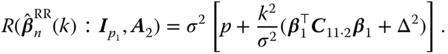
- Restricted ridge estimator (RRRE)
(6.92)

Then, the
 ‐risk of
  is(6.93)
Now consider the following weighted risk function:

Thus,
(6.94)
- Preliminary test ridge regression estimator (PTRRE)
The bias and weighted risk functions of PTRE are respectively obtained as follows:
(6.95)
The weighted (weight,
 is obtained as follows:(6.96)
- Stein‐type ridge regression estimator (SRRE)
The bias and weighted risk functions of SRRE are respectively obtained as follows:
(6.97)
The weighted (
 ) risk function of the Stein‐type estimator is obtained as follows(6.98)
- Positive‐rule Stein‐type ridge estimator (PRSRRE)
The bias and weighted (
 ) risk functions of PTSRRE are, respectively, obtained as follows:(6.99)
where

6.10.3 Comparison of the Estimators
Here, we compare the URE, SRE, and PRSRRE using the weighted ![]() ‐risks criterion given in Theorem 6.3.
‐risks criterion given in Theorem 6.3.
6.10.4 Asymptotic Results of RRE
First, we assume that
where for each ![]() ,
, ![]() are i.i.d. random variables with mean zero and variance
are i.i.d. random variables with mean zero and variance ![]() . Also, we assume that
. Also, we assume that ![]() s satisfy
s satisfy

for some positive definite matrix ![]() and
and
Suppose that

and define ![]() to minimize
to minimize

Then, we have the following theorem from Knight and Fu (2000).
This theorem suggests that the advantages of ridge estimators are limited to situations where all coefficients are relatively small.
The next theorem gives the asymptotic distribution of ![]() .
.
From Theorem 6.5,

where ![]() .
.
6.11 Summary and Concluding Remarks
In this chapter, we considered the unrestricted estimator and shrinkage estimators, namely, restricted estimator, PTE, Stein‐type estimator, PRSE and two penalty estimators, namely, RRE and LASSO for estimating the regression parameters of the linear regression models. We also discussed about the determination of the tuning parameter. A detailed discussion on LASSO and adaptive ridge regression estimators are given. The optimization algorithm for estimating the LASSO estimator is discussed, and prostate cancer data are used to illustrate the optimization algorithm.
Problems
- 6.1
Show that
 approaches singularity as the minimum eigenvalue tends to 0.
 - 6.2 Display the graph of ridge trace for the Portland cement data in Section 6.5.
- 6.3 Consider the model,
 and suppose that we want to test the null‐hypothesis
  (vs.)
(vs.)  . Then, show that the likelihood ratio test statistic is

which follows a noncentral
 ‐distribution with
  DF and noncentrality parameter,
  .
. - 6.4 Similarly, if we want to test the subhypothesis
 vs.
vs.  , then show that the appropriate test statistic is,

where

and
 ,
,  .
. - 6.5
Show that the risk function for GRRE is
(6.112)

- 6.6 Verify (6.60).
- 6.7 Verify (6.74).
- 6.8 Consider a real data set, where the design matrix elements are moderate to highly correlated, then find the efficiency of the estimators using unweighted risk functions. Find parallel formulas for the efficiency expressions and compare the results with that of the efficiency using weighted risk function. Are the two results consistent?