Chapter 13
Extensions of Multiple Regression
Chapter 12 provided an introduction to multiple regression, and this chapter continues that discussion. In particular, we consider the use and effect of dummy variables in multiple regression, the selection of best models in multiple regression, correlation among independent variables and the effect of this correlation, and the assessment of nonlinear relationships.
13.1 Dummy Variables in Multiple Regression
Chapter 11 discussed the correspondence between regression and the t test. That chapter also showed that the results of both analyses were essentially the same when a dummy variable alone was employed as the predictor variable in regression. This section examines the inclusion of a dummy variable, along with other continuous variables in multiple regression analysis, to produce what is sometimes called analysis of covariance (ANCOVA).
A Dummy Variable with No Interaction
Suppose we examine again the data shown in Figure 11.3. Those data show 20 hospital stays and the total charge for each. But this time we will include a second variable: sex of the patient. The length of stay and charges data were taken from actual hospital discharge records. However, the included sex variable was made up to fit the example we will discuss. The new data set for the 20 discharges is shown in Figure 13.1, and it shows the length of stay as x1 and sex as x2. It should be clear that sex is a categorical variable that has been labeled 1 and 0 (1 = female; 0 = male). This allows the categorical variable sex to be treated as a numeric variable in regression (as shown in Chapter 11).

Figure 13.1 Data for 20 hospital days with sex as a dummy variable
Now, if the regression coefficients for the two independent variables and the intercept are calculated for these data, the results are as shown in Figure 13.2. It can be seen in the figure that the coefficients for both length of stay and sex are different from 0, according to the t tests and probabilities of t (cells K18 and 19 and L18 and 19, respectively).

Figure 13.2 Results of regression for 20 hospitals
The Equation for Predicted Values of Total Costs
With the results shown in Figure 13.2, the equation for the predicted values of total charges (TC), given the length of stay and the sex of the patient, is as shown in Equation 13.1. But because sex takes on only the two values 1 and 0, the predicted values of total charges actually form two lines—one when the categorical variable sex is coded 0 (male) and one when sex is coded 1 (female). The equation of these two lines is as shown in Equation 13.2. The parts within the parentheses in Equation 13.2 are read TCpred, given that sex equals 0 (male), and TCpred, given that sex equals 1 (female).

It should be clear that these two lines are exactly parallel to each other (they have the same slope of $875.05) and are exactly $1,544.55 apart ($1688.25 − $143.70). The predicted lines for male and female patients among the 20 in the data set are shown in Figure 13.3. Also shown in the figure are the actual observations. The observations for women are shown as black diamonds and for men as gray squares. As the two parallel predictor lines show, the cost goes up by $875.05 per day, but for every day, the cost is higher for women than for men by $1,544.55. It might also be noted that the two regression lines defined by the equations in Equation 13.1 and Equation 13.2 account for 92 percent of the variance in total charges ![]() .
.

Figure 13.3 Graph of cost data by length of stay
General Formula for Multiple Regression Analysis Using a Dummy Variable
Having looked at the effect of a single dummy variable added to a regression analysis, it is useful to provide a general formula for the effect of a dummy variable alone in a multiple regression model. This is shown in Equation 13.3.
then
and
where D is the dummy, and bD is the coefficient of the dummy.
The Interaction Effect
When a dummy variable is included in regression, the effect of the dummy could be more complex than simply to define two parallel regression lines. It is possible that the two lines (or planes, or hyperspaces) defined by the dummy variable may not be parallel. But for this to occur, the regression analysis would have to include not only the dummy variable but also an interaction term between the dummy variable and at least one continuous variable.
Consider again the data for hospital charges shown in Figure 13.1. Now include an interaction between the continuous variable length of stay and the dummy variable sex, as shown in Figure 13.4. In that figure, it can be seen that the interaction is simply the multiplication of the continuous variable by the dummy variable. When the dummy variable is 0, the interaction term (x1*x2) is 0. When the dummy variable is 1, the interaction term is equal to the continuous variable.

Figure 13.4 Hospital charges with dummy and interaction
We now carry out regression analysis with charges as the dependent variable and the three independent variables as shown in Figure 13.4. The resulting regression coefficients, their standard errors, and the appropriate t tests are shown in Figure 13.5. These regression coefficients also account for 92 percent of variance. The fact that the interaction term adds nothing to the regression equation in terms of the variance accounted for is confirmed by the t statistic for the interaction term, shown in cell L40. The t statistic is 0.55, which has a 59 percent probability of occurrence under the null hypothesis that charges are independent of the interaction between the length of stay and sex. In essence, we conclude that the coefficient on the interaction term is 0.

Figure 13.5 Regression coefficients with dummy and interactions
A Dummy Variable with an Interaction
We now consider an example in which the interaction term is statistically significant. In other words, can we conclude that the coefficient on the interaction term is different from 0? Such an example is shown in Figure 13.6. This figure shows the same charges and the same length of stay as those shown in Figures 13.1 and 13.4. However, the sex designations have changed to present a different picture of the data. If regression is carried out using only the dummy variable with no interaction term, the results are as shown in Figure 13.7.

Figure 13.6 Hospital charges with dummy and interaction: Modified example
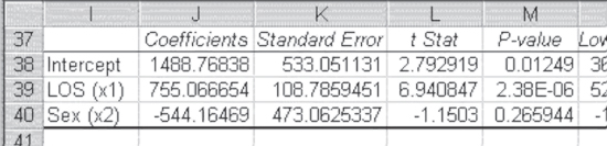
Figure 13.7 Regression coefficients with dummy only: Modified example
Of the regression coefficients shown in Figure 13.7, only the coefficients for length of stay and the intercept are different from 0. Sex is no longer a statistically significant predictor of charges. In this case, it would be a reasonable practice to simply drop sex from the analysis and predict charges with the length of stay only, except for one thing. It may be that the interaction between the length of stay and sex could have a statistically significant relationship to charges. To determine if it does, it would be necessary to analyze all three variables—the length of stay, sex, and the length of stay/sex interaction—simultaneously. The coefficients that result from this analysis are shown in Figure 13.8. In that figure it is possible to see that not only is the coefficient for sex statistically different from 0, but so, too, is the interaction coefficient.

Figure 13.8 Regression coefficients with dummy and interaction: Modified example
In addition, the coefficient on the length of stay remains statistically significant. What does this mean in terms of the prediction of charges? It means not only will charges be predicted by two lines with different intercepts for males and females, but also the slopes of those lines will be different. This can be seen in the equations for the two lines, as shown in Equation 13.4. For men ![]() , the charge increases by $637.51 for each additional day of stay, with a fixed cost of $1,959.01 for a stay of zero days. For women, the cost increases by $1,305.35 per day of stay from a fixed cost of
, the charge increases by $637.51 for each additional day of stay, with a fixed cost of $1,959.01 for a stay of zero days. For women, the cost increases by $1,305.35 per day of stay from a fixed cost of ![]() for a stay of zero days. Of course, because no hospital admission will be a zero-day stay, the intercept terms represent only the y-axis anchor for the respective lines.
for a stay of zero days. Of course, because no hospital admission will be a zero-day stay, the intercept terms represent only the y-axis anchor for the respective lines.
or
and
Now that we have seen that the regression lines are different, it may be useful to see how these are pictured in a two-dimensional graphic presentation. Figure 13.9 shows the graph of the charges data with the two regression lines as defined by Equation 13.4, included in the graph. The more steeply sloped graph with the intercept below 0 is the line for women. The actual observations for women are shown as diamonds. The less steeply sloped graph with the regression line crossing the y-axis at about $2,000 is the slope for men. The actual observations for men are shown as squares.

Figure 13.9 Hospital charges with dummy and iteration graphed
It should be remembered that these examples, although based on actual charge and length of stay data, have fabricated data for sex. The sex variable has been manipulated in each case just presented to produce the outcomes that have been found. It is highly unlikely that over a large sample of data any difference would be found for men and women in hospital charges. In addition, the result of an interaction effect would be even more unlikely. Nevertheless, there are many situations in which dummy variables and interaction terms could have realistic meaning. With that in mind, it is useful to present a general formula for determining the slope and intercept of lines when dummy variables and interactions are present. Such a formula is given in Equation 13.5.
then
and
where D is the dummy, and bD is the coefficient of the dummy.
If there is more than one continuous independent variable, the slope of the line defined by the continuous variable will change only for those variables for which there are dummy continuous variable interaction terms.
General Comments on Dummy and Interaction Terms
Let's assume that an interaction is expected and an interaction term is included in an analysis with a continuous variable and a 1/0 dummy. In turn, the full regression model, including the interaction term, should be run. If the interaction term is not different from 0 (i.e., if the absolute t value is less than 2), the interaction term can be dropped. Then the analysis can be rerun with only the continuous variable and the dummy variable included. This simpler model will describe the data as adequately as the more complex model, including the interaction. If, in this further analysis, the coefficient for the dummy is not different from 0, it is possible to drop the dummy as well and simply predict the dependent variable on the basis of the continuous variable (or continuous variables).
Let's now assume that an interaction term is included in an analysis and the coefficient for the interaction term is different from 0 but the coefficients for the continuous variable and the dummy variables are not different from 0. A similar decision as previously mentioned may be made. It is sometimes possible to drop the continuous variable and the dummy variable and predict the dependent variable solely on the strength of the interaction variable itself. The results of the analysis may produce slightly different coefficients, but the predicted values of the dependent variable will be very much the same.
Example of Using Only the Interaction Term as the Predictor
To see an example of this, consider the imaginary hospital charge data shown in Figure 13.10. In this data set, Inpatient=1 means that the patient was actually in the hospital during the length of stay indicated, whereas Inpatient=0 means that the patient was being treated during the time period indicated as LOS (length of stay) on an outpatient basis. The question is whether there is an interaction effect of LOS and Inpatient.

Figure 13.10 Charge data showing an interaction effect
Using the Data Analysis ⇨ Regression add-in produces the coefficients shown in Figure 13.11. In that figure it can be seen by the t tests on the three coefficients representing the independent variables and the probabilities of those t tests (cells M18:M20 and N18:N20, respectively) that only the coefficient for the interaction is different from 0. This essentially means that neither the continuous variable LOS nor the dummy variable Inpatient contributes in a statistically significant way to the prediction of charges. The total proportion of the variance in charges accounted for by all three variables (R2) is 0.91.

Figure 13.11 Coefficients for charge data showing an interaction effect
Because neither the coefficient on LOS nor that on Inpatient is statistically different from 0 in the analysis of the data in Figure 13.10, it is not unreasonable to consider dropping those from the analysis in order to predict charges.
Conceptually, this amounts to imputing a fixed fee to outpatient contacts with the hospital. This result is regardless of the amount of time over which they extend, and in turn predicting inpatient stays on the basis of the time in the institution. The result of this analysis is shown in Figure 13.12. Here, the coefficient for the interaction has changed from 230.39 (Figure 13.11) to 270.61, but the total proportion of the variation accounted for remains essentially at 0.91. In essence, either model is equally good at predicting hospital charges as represented by the data in Figure 13.10.

Figure 13.12 Coefficients for charge data showing only the interaction effect
Graphing the actual data points and both predicted values for the data, those using the coefficients in Figure 13.11 and those using the coefficients in Figure 13.12, will show this. The result is shown in Figure 13.13.

Figure 13.13 Graph of charge data with predicted lines
Comparison of Models in Graphical Form
In Figure 13.13, the gray squares represent charges for actual hospital stays. The black diamonds represent charges for outpatient contacts with the hospital over the numbers of days indicated on the horizontal axis. Turn your attention to the sloping line from about 2360, when days of contact with the hospital are zero, to about 2800, when days of contact with the hospital are 12. It represents the predicted charges for those who were treated on an outpatient basis when the predicted values are calculated using all three coefficients (refer to Figure 13.11).
The horizontal line at 2643 represents the predicted charges for those people who were treated on an outpatient basis, using only the coefficients given in Figure 13.12. The line is essentially the mean of the outpatient charges. This occurs because there is no separate term to represent the length of contact with the hospital for the outpatient group.
Focus next on the diagonal line sloping from about 2600, when length of stay is zero days, to about 5700, when length of stay is 12 days. This line represents the predicted value of charges for those people who actually had hospital stays, using either set of coefficients. The lines are so close together that they cannot be shown separately on the graph. (The predicted line given the coefficients in Figure 13.11 is Charges = 274.05 LOS + 2,616.35, whereas for the coefficients in Figure 13.12, it is Charges = 270.61 LOS + 2,643.27.)
In considering the preceding discussion, an important point should be noted. Dropping both the slope and intercept terms and predicting the charges values simply on the basis of the interaction assume automatically that the outpatient contacts (given as 0 in the dummy variable) actually have no relationship to number of days of contact with the hospital. If they did, the coefficients for days and the intercept would have had to be included in the analysis, even if they were not statistically different from zero. Otherwise, the predicted values for charges for outpatients would always be a flat line.
13.2 The Best Regression Model
The discussion in Section 13.1 focused on dummy variables and their treatment in regression. In that discussion there exists the question of whether to include a dummy variable or an interaction term in a general regression model. The decision to include was based on whether either was not statistically significant (i.e., different from 0). The conclusion from the discussion was that it did not make much difference either way in the prediction of the dependent variable.
In general, that result holds. However, the question of whether it is appropriate to drop variables from a regression model if they are not statistically significant is one that is widely debated. There is no generally accepted agreement on which is correct.
Theory or Dust Bowl Empiricism?
The argument for dropping statistically nonsignificant variables from a regression model is based on two points. First, including statistically nonsignificant variables in a model will not improve the prediction of the dependent variable in any statistically significant way. Second, including statistically nonsignificant variables unnecessarily complicates the understanding of the dependent variable with extraneous independent variables that have no predictive value.
The argument for not dropping statistically nonsignificant variables from a regression model is based primarily on a single point, but it is an important one. This point is that a regression equation implies a causal relationship in which the values of the dependent variable are actually caused by the values of the independent variable set.
This causal relationship in turn implies some underlying theoretical model that says a certain set of independent variables should be included in a regression model. The fact that in a particular instance under analysis this may not have been found to be true does not necessarily invalidate the theory. Neither does it allow the analyst to drop a variable from the predictor model. To do so is not only to abandon the theory but, as we have seen in regard to dummy variables, also to change the values of the coefficients.
The argument that a regression model represents a theory is further supported by the empirical evidence that one set of predictor variables may be as useful as another completely different set of predictor variables in predicting a dependent variable. In such a situation, only a theory, and not simply the regression analysis alone, can determine which variables to include in the regression equation.
To Drop Regression Variables or Not to Drop Regression Variables: An Exploration
To explore some of these issues, we will use data taken from The State of the World's Children 1996 ([1996]). These data are for 75 countries in the world for which all the data to be examined were available. (It should be noted that UNICEF publishes these data every year, so more recent data are available. The data from [1996] demonstrate several points that are to be made in this section, whereas data from later years do not necessarily demonstrate the same points. One of the difficult things about regression analysis is that the data do not always behave in the same ways from one sample to another.)
A sample of the data under consideration is shown in Figure 13.14. The data represent eight independent variables and one dependent variable. The dependent variable is U5Mort in column K, the under-five mortality for each country for 1994. The eight independent variables include five variables related to the public health system.

Figure 13.14 Data from The State of the World's Children [1996]
The variable SafeW is the proportion of households with access to safe water. The variable Sanit is the proportion of households with access to sanitary facilities. The variable HealthS is the proportion of households within a specified travel distance of a health facility. The variable DPT is the proportion of children immunized for diphtheria, pertussis, and tetanus by age one. The variable CPR is the contraceptive prevalence rate.
Also included as independent variables are three that are not dimensions of the health care system. The variable LogGNP is the log of the gross national product per capita (the log is used because the actual value of GNP is not linearly related to under-five mortality, whereas the log is). The variable FemLit is the female literacy rate for the country. The variable TFR is the average number of births per woman.
Each one of the independent variables in Figure 13.14 is approximately linear in its relation to U5Mort. In addition, each is a statistically significant predictor of U5Mort. Figure 13.15 is a composite of eight separate regression analyses, one for each of the independent variables predicting U5Mort on its own.

Figure 13.15 Coefficients for each of the predictor variables for U5Mort independently
As the t statistics and their probabilities indicate (columns AJ and AK, respectively), each of the independent variables, taken separately, is a statistically significant predictor of under-five mortality. Furthermore, take a look at the R2 value, shown in column AM. R2 indicates that the independent variables, taken alone, account for between 43.7 percent (for HealthS) and 71.6 percent (for CPR) of the variance in under-five mortality across the data set.
Consider first the question of what to do about statistically nonsignificant variables in a multiple regression model. To do this, we will look at all eight of the independent variables shown in Figures 13.14 and 13.15, analyzed simultaneously. The result of this analysis is shown in Figure 13.16.

Figure 13.16 Multiple regression coefficients of predictors for U5Mort
As Figure 13.16 shows, when all seven independent variables are included in the regression model, only one coefficient, that for Sanit, is different from 0 (i.e., a probability of less than 0.05). This is despite the fact that when each variable is examined separately in regard to under-five mortality, each of the eight has a nonzero coefficient. The total variance accounted for (R2) by all eight variables in the regression model (even though only one is statistically different from 0) is 0.815.
Comparing Models with and without Variables: Stepwise Regression
Within the context of the view that holds that a theory must be the basis of the regression model analyzed, it would have been assumed that some theory specified that all eight variables should be included in the multiple regression model. Within this perspective, the fact that only one variable (Sanit) actually shows a statistically significant coefficient would not be sufficient cause to eliminate any of the variables used as a way to simplify the regression model. Within the context of the alternative view, which seeks the simplest regression model for predicting the dependent variable, it is clear that some variables in the model are not useful and should be dropped. One approach to this would be simply to fall back to the use of Sanit alone to predict U5Mort. But we already know that Sanit alone is not the best predictor of U5Mort, that distinction being held by CPR (see Figure 13.15). So, how should we proceed?
A common approach to seeking the best multiple regression model is what is often called stepwise regression, a term that denotes a number of different methods. These methods vary in their levels of complexity for seeking the best set of independent variables for simultaneously predicting the dependent variable of interest. In general, the various stepwise regression approaches can be characterized as either backward stepwise elimination or forward stepwise inclusion.
Backward Stepwise Elimination
The simplest example of backward stepwise elimination begins with the complete model, as shown in Figure 13.16. It then successively eliminates in a stepwise manner the predictor with the least significant coefficient. This process continues until only variables with statistically significant coefficients remain. If the backward elimination approach to stepwise regression is employed, the first variable to be eliminated is SafeW, with a P-value of 0.928. Although the result of that analysis with six independent variables is not shown, the next variable to be eliminated would be TFR. The stepwise process would continue until only variables with statistically significant coefficients remain.
Figure 13.17 shows the results of the backward elimination process beginning with all variables shown in Figure 13.16. As Figure 13.17 shows, four variables—LogGNP, Sanit, DPT, and CPR—have coefficients that are statistically different from 0 after the stepwise procedure. The resulting R2 is 0.798.

Figure 13.17 Multiple regression coefficients of best predictors for U5Mort: Backward elimination
Forward Stepwise Inclusion
Forward stepwise inclusion begins with the single variable that accounts for the largest proportion of the variance and proceeds at each step by adding a next variable that accounts for as much of the unexplained variance as possible. This essentially means selecting the next variable that, with the two variables taken together, accounts for the largest proportion of variance (has the largest R square). From the forward inclusion approach, the first variable into the model would be CPR. CPR accounts for the largest proportion of variance in under-five mortality when each variable is taken singly (R2 = 0.716 in Figure 13.15). With CPR included, the next best predictor is Sanit. Together, CPR and Sanit account for 0.768 percent of the variance in U5Mort. With CPR and Sanit included, the next best predictor turns out to be TFR. When TFR is included with CPR and Sanit, they account for 0.789 percent of the variance in U5Mort.
But now a problem arises in the analysis. When TFR is included with CPR and Sanit, the coefficient for CPR is no longer different from 0 (i.e., the probability for the t statistic is greater than 0.05—actually, 0.068). This requires a decision that, in general, does not usually arise with backward elimination. We can continue with CPR, Sanit, and TFR, even though CPR is no longer statistically different from 0. On the other hand, we could drop CPR, replace it with TFR, and continue to develop the model on the basis of TFR and Sanit. In this case, we will elect the latter approach.
The results of the forward inclusion method (substituting TFR for CPR because when TFR, CPR, and Sanit are included in the same model, CPR no longer has a coefficient different from zero) are shown in Figure 13.18. Three variables—TFR, Sanit, and DPT—have coefficients different from zero. Adding any other variable to this set of three results in a probability greater than 0.05 for the coefficient of the added variable. This model, with three predictor variables, accounts for 79.6 percent of the variance in U5Mort.

Figure 13.18 Multiple regression coefficients of best predictors for U5Mort: Forward inclusion
Backward Elimination or Forward Inclusion: Which Method to Choose?
It is possible that with a more sophisticated approach to backward elimination, both approaches would have reached the same result as shown in Figure 13.18. But a more sophisticated approach to forward inclusion, regardless of how good any single one was, might have also resulted in a different set of predictor variables—for example, selecting the best three predictors simultaneously.
The bottom line is this: In general, stepwise regression, though it may result in a simplified model, is probably less desirable as an approach to regression analysis than analysis based on a clear understanding of which independent variables should be included in a given model. This can be determined only from a clear understanding of the process that actually produces the results in the dependent variable of interest. The best place to obtain this understanding is a good theory.
Stepwise Regression in Excel
Dedicated statistics packages often have a few commands that will allow the user to perform a host of forward, backward, and sideways regression analyses (the sideways regression analysis is problematic), producing vast reams of printout. Microsoft Excel, though an outstanding statistical tool, does not produce stepwise regression results quite so easily. It is necessary with Excel to do each regression separately. So, if one is to replicate the discussion in the previous (first) subsection of this section (13.2), as is suggested in Exercise 1 of this section, a little direction is probably useful.
Single-Variable Regression Using Excel
To replicate the results in the previous discussion, begin with the data on the U5Mort1 worksheet of Chpt 13-1.xls. The first task is to reproduce the single-variable regression results shown in Figure 13.15. Begin with the data on the U5Mort1 worksheet, which are those given in Figure 13.14. Using Data Analysis ⇨ Regression, specify U5Mort as the dependent variable and SafeW as the independent variable. Specify the output cell as M1. This will produce the regression that will allow you to replicate row 2 in Figure 13.15. Now recall the Data Analysis ⇨ Regression dialog box, and change the independent variable to Sanit and the output cell to M21. This will cause the result to replicate row 3 in Figure 13.15. Proceed this way with the remaining six variables, putting the results in M41, M61, M81, and so on. This allows you to produce all of the results shown in Figure 13.15.
Backward Elimination Using Excel
To replicate the results in Figure 13.16, the entire independent variable set from SafeW to TFR should be included in a single regression model. Because this is the first step to the backward elimination process, insert a new worksheet, label it U5Mort1-b for backward elimination, and copy the data in cells A1:K76 to the new worksheet. Now invoke Data Analysis ⇨ Regression, and specify all the variables from SafeW to TFR as the independent variables. Put this result in cell M1. This replicates Figure 13.16 and also provides the starting point for backward elimination.
As the analysis in Figure 13.16 shows, SafeW has the smallest p value in the complete model. This is the first variable to be eliminated in the next step. Copy all the data from cells D1:J1 (i.e., all the independent variables except for SafeW), and paste the copy into cell W1. This now leaves seven independent variables in columns W through AC. Invoke Data Analysis ⇨ Regression again, and change the variable fields to reflect the moved data set. (It is necessary only to change the reference for the independent variables, because the dependent variable remains in column K.) Put the result into cell AE. In this analysis you will discover that TFR has the largest p value (0.275) and is the next to be eliminated.
Copy the six independent variables (columns W to AB), and paste them into cell AO1. This eliminates TFR. Now invoke Data Analysis ⇨ Regression, specify the new set of six independent variables, and specify the output cell as AV1. In this analysis you will discover that HealthS has the largest p value (0.137) and will be the next variable eliminated. The easiest way to do this is to copy all the columns AO through AT and paste them into cell BF1. Then click the BG at the top of the HealthS column, and eliminate the entire column. This will now put the five remaining independent variables into columns AO:BJ. Analysis proceeds in this fashion until all variables in the model have p values of 0.05 or less, at which time the regression analysis result should look exactly like that in Figure 13.17 (it will take two more steps, and the variables will not appear in the same order, but the coefficients, t tests, and p values will be the same).
Forward Stepwise Inclusion Using Excel
Replicating forward stepwise inclusion to produce the result shown in Figure 13.18 is a similar, but somewhat more complicated, process. To begin the process, return to the U5Mort1 worksheet on which the regressions with each independent variable as a predictor of U5Mort were carried out. Then select the variable with the largest R2 value. This happens to be CPR (shown in Figure 13.15).
Copy the variable CPR to column W, beginning in cell W1. Now select the first of the other independent variables, SafeW, and copy it to column X, beginning in cell X1. Now invoke Data Analysis ⇨ Regression, and specify the two variables CPR and SafeW in columns W and X, respectively, as the independent variables. Put the results into cell Z1. Now it is time to pair CPR with Sanit.
Recall that it is necessary for the entire independent variable set in regression to be in contiguous columns. So Sanit must be contiguous with CPR. The easiest way to do this is to click the X that heads the column containing SafeW and insert a new column at this point. This moves the variable SafeW to column Y and the output from the most recent regression to column AA. Now copy the data for Sanit, and put it into column X, beginning in cell X1. Using the variables CPR and Sanit, replicate the previous regression and put the output into cell AA21. In doing this, it will be necessary to change only the destination cell.
To continue with the two-variable regression, continue to add a new column at X for each new variable to be paired with CPR until all the other six variables have been analyzed this way. It should not ever be necessary to change the data references, but it will be necessary to change the output reference each time to ensure that all the output is in the same column. The cell into which the last regression output will go for this sequence (which will be the pairing of CPR with TFR if you are following this example) will be cell AF121.
After completing this sequence of two variables, you will see that CPR and Sanit, taken together, have the largest R2 at 0.768. So these two variables will be those included at the next step. This next step will proceed just as the last did, except that now the two variables—CPR and Sanit—will be copied to the columns AP and AQ, beginning in the first cell in those columns. Now the first of the remaining variables, SafeW, will be copied to column AR, and a new regression analysis will be performed with these three variables as the predictors. It will be necessary to change the x input range to reflect the three variables being analyzed, and also the output range, which should be specified as cell AT1.
Just as in the previous sequence, we now insert a column at AR and copy the next variable, HealthS, to that column. Now that we've done this, regression is again performed, changing only the output destination to AU22. Another column is inserted at AR, and the process continues. The destination of the last regression analysis will be cell AY106.
Having completed this stage of the analysis, we will see that the largest R2 (0.789) is associated with regression that includes CPR, Sanit, and TFR. But as noted previously, CPR no longer has a statistically significant coefficient (p = 0.068). So we will drop CPR in favor of TFR and replicate the two-variable analysis with Sanit and TFR.
In the repeat of the two-variable analysis with Sanit and TFR, it turns out that only one of the other six variables, DPT, has a coefficient different from 0, and that is the last variable to be included. This set of three variables accounts for 79.6 percent of the variance (R2 = 0.796), and the analysis is complete.
An Alternative Look at the Importance of Theory
This concern with a theoretical approach to regression is also supported with a somewhat different analysis of these same data. Suppose we have one group of analysts who believe that the important determinant of under-five mortality is the health and health services environment of a country. With that in mind, they might reasonably decide to predict under-five mortality by using those available variables that are health-related, which, in this case, could include the variables SafeW, Sanit, HServe, DPT, and CPR. Another group of analysts might believe that the important determinant of under-five mortality is not the health environment of the country but, rather, the general cultural environment. Therefore, they might determine that they should predict under-five mortality by using the cultural variables FemLit, LogGNP, and Fert.
Taking the health approach, and using backward elimination of nonsignificant coefficients, the results of the analysis are shown in Figure 13.19. The three variables, Sanit, DPT, and CPR, together account for 78.3 percent of the variance in under-five mortality. If the general cultural environment approach is taken, the results of the analysis are shown in Figure 13.20. Here, all three variables had statistically significant coefficients on the first analysis. The three variables, LogGNP, FemLit, and Fert, taken together account for 73.6 percent of the variance in under-five mortality. It is possible to account for similar proportions of the variation in under-five mortality, approaching it as strictly a health issue, or as a cultural issue. The bottom line is that the statistical analysis alone is a weak tool for deciding which variables should or should not be included in the analysis.

Figure 13.19 Multiple regression coefficients of best predictors for U5Mort: Health predictors

Figure 13.20 Multiple regression coefficients of best predictors for U5Mort: Cultural predictors
Despite the problems of determining the correct regression model on the basis of the statistical analysis alone, there will continue to be those who use the stepwise method—either forward or backward or both—to uncover the “best” regression models. There will also continue to be many who say that the regression model can be determined only by a theoretical framework and confirmed or not confirmed by the analysis.
Perhaps the best that can be said about the two approaches is that the former is largely exploratory, whereas the latter is an attempt at the confirmation of theory. Short of that, the controversy is not likely to be resolved.
13.3 Correlation and Multicolinearity
How is it that different independent variables can produce similar results in predicting a dependent variable? Or how is it that two variables can each separately predict 50 percent or more of the variance in an independent variable but together cannot predict more than 70 percent? The answer is that the predictor variables themselves are related. This is frequently called multicolinearity. Multicolinearity has two effects in multiple regression analysis—one is of little consequence and the other is of some significant consequence. The first result is what we have already seen: the result that different variables can produce similar results as predictors of a dependent variable and that the proportion of variance attributable to two variables taken together will not generally be the sum of the variance attributable independently by each. The second result—that of some consequence—is that as colinearity increases, the standard errors of the coefficients that are multicolinear will increase. This can result, for example, in two variables that are both statistically significant predictors of a third variable when taken independently, with neither being statistically significant when examined together.
Examining Multicolinearity
To examine multicolinearity, consider first the relationship between the independent variables examined in Section 13.2, the eight variables taken from The State of the World's Children 1996 ([1996]). Figure 13.21 shows the correlation between the eight predictors of U5Mort. This was generated using the Excel add-in for correlation in Data Analysis ⇨ Correlation. A correlation is exactly the same as the value of Multiple R in regression analysis that would be generated if only one independent variable were considered at a time. You will recall that the Multiple R is just the square root of R square. So the correlations shown in Figure 13.21 are essentially the square roots of the amount of variance shared between each of the variables shown. For example, the correlation between SafeW and Sanit (cell M4) is 0.668. This means that SafeW and Sanit share about 44.7 percent of their variance ![]() .
.

Figure 13.21 Correlation among the predictors for U5Mort
Calculating the Correlation Coefficient
Thus far, the correlation between two variables has been computed either by using the correlation add-in in Data Analysis or as the Multiple R in regression. The correlation coefficient can be calculated directly by using the formula given in Equation 13.6, where x refers to one of the two variables and y refers to the other.

If the correlation table in Figure 13.21 is examined closely, it is possible to see that the highest correlation is between CPR (contraceptive prevalence rate) and TFR (total fertility rate) (0.914 in cell Q10). There is every reason to expect that these two variables would be highly correlated. Therein is reason to believe that higher contraceptive prevalence rates will actually produce lower total fertility rates. If these two variables are examined independently with regard to U5Mort, CPR accounts for 71.6 percent of the variance in U5Mort and TFR accounts for 66.8 percent (Figure 13.15). Both variables have statistically significant coefficients ![]() .
.
Considering Variables Simultaneously: A Test for Standard Error Inflation
Now consider what happens if the two variables are considered simultaneously. The result of the simultaneous analysis of CPR and TFR produces the coefficients and t tests shown in Figure 13.22. Now, the two variables together account for 72.8 percent of the variance in U5Mort, but TFR is no longer statistically different from 0 ![]() . Furthermore, the probability for CPR now reaches only 0.0002. Is there a better demonstration of the effect of multicolinearity as an inflator of standard errors? To find one, it is necessary to modify the data a little.
. Furthermore, the probability for CPR now reaches only 0.0002. Is there a better demonstration of the effect of multicolinearity as an inflator of standard errors? To find one, it is necessary to modify the data a little.

Figure 13.22 CPR and TFR together as predictors for U5Mort
CPR and TFR are highly correlated—that is, 0.914, which means they share about 83 percent of their variance ![]() . But the effects of extreme multicolinearity do not arise at that level. To see the effects, it is necessary to increase the relationship between CPR and TFR. To do that, 31 countries that had the lowest correlations between CPR and TFR were removed from the data set, resulting in 44 countries for which CPR and TFR were correlated at 0.962. At that level of correlation, they share about 92 percent of their variance. When each of the variables is separately related to U5Mort, the results are quite like those in Figure 13.15. The probability of the coefficient for CPR is 2.76E-12, and the probability of the coefficient for TFR is 2.36E-12. Each of the variables independently accounts for about 69 percent of the variance in U5Mort. But when they are examined simultaneously, the results are as those shown in Figure 13.23. It can be seen there that neither coefficient (CPR or TFR) has a statistically significant probability. This is the consequence of extreme multicolinearity. It inflates the standard errors to the extent that variables no longer show statistical significance. But it is important to note that this happened at a correlation between CPR and TFR of 0.962.
. But the effects of extreme multicolinearity do not arise at that level. To see the effects, it is necessary to increase the relationship between CPR and TFR. To do that, 31 countries that had the lowest correlations between CPR and TFR were removed from the data set, resulting in 44 countries for which CPR and TFR were correlated at 0.962. At that level of correlation, they share about 92 percent of their variance. When each of the variables is separately related to U5Mort, the results are quite like those in Figure 13.15. The probability of the coefficient for CPR is 2.76E-12, and the probability of the coefficient for TFR is 2.36E-12. Each of the variables independently accounts for about 69 percent of the variance in U5Mort. But when they are examined simultaneously, the results are as those shown in Figure 13.23. It can be seen there that neither coefficient (CPR or TFR) has a statistically significant probability. This is the consequence of extreme multicolinearity. It inflates the standard errors to the extent that variables no longer show statistical significance. But it is important to note that this happened at a correlation between CPR and TFR of 0.962.

Figure 13.23 CPR and TFR together as predictors for U5Mort: Reduced sample
In general, multicolinearity is not a problem to be concerned about unless the correlation between variables exceeds about 0.90.
13.4 Nonlinear Relationships
Up to this point, we have considered regression analysis in its classical context. We examined the linear relationships between independent and dependent variables. But regression analysis can also be used in certain cases to analyze nonlinear relationships. This section discusses some of the ways in which Excel can be used to perform nonlinear regression analysis.
Estimating a Nonlinear Relationship
In examining the relationship between the independent variables taken from The State of the World's Children 1996 and U5Mort, LogGNP, rather than GNP itself, was used as a predictor, because it was indicated that GNP is not linearly related to U5Mort, whereas LogGNP is. This decision deserves somewhat more discussion and some observations on the analysis of nonlinear relationships. To begin the discussion it is useful actually to look at the relationship in an xy graph.
A graph of the relationship between GNP and U5Mort is shown in Figure 13.24. It is possible to see that the relationship is decidedly nonlinear. Below a GNP of about $5,000 per year, U5Mort falls precipitously from over 300 to below 50. For the four countries above $5,000 per year, the differences in U5Mort are comparatively small. Although a straight line might fit the data either below or above $5,000, a straight line does not fit both segments of the data simultaneously.

Figure 13.24 Relationship between GNP and U5Mort
Fitting Nonlinear Relationships Using Second-Degree Curves
There are a number of different ways to attempt to fit the data represented by the relation between GNP and U5Mort. Consider first the possibility of fitting the line with a second-degree curve. In general, a second-degree curve is any relationship between a dependent and an independent variable that is defined by the independent variable and a power of the independent variable. But, typically, a second-degree curve is defined by the original independent variable and its square.
A major characteristic of a second-degree curve is that it produces a graphed line that has one change of direction. In Figure 13.24, the data essentially change direction one time. This direction change occurs at about 25 deaths per 1,000 live births or at about $1,500 in GNP per capita. A third-degree curve would have two changes of direction, a fourth-degree curve would have three, and so on. In general, data that are encountered in health care–related applications will rarely benefit from going beyond a second-degree curve.
A sample of the data (for the first 10 countries) for analyzing the relationship in Figure 13.24 is shown in Figure 13.25. Column B is the actual value of GNP per capita, and column C is the square of GNP per capita. Column D is the actual value of U5Mort, and column E is the best-fitting second-degree curve through the data.

Figure 13.25 Sample of data for second-degree curve analysis of U5Mort
The actual regression equation that predicts that curve (which was found by using Data Analysis ⇨ Regression) is shown in Equation 13.7. This equation accounts for 39.6 percent of the variance in U5Mort (R2 = 0.396), compared with only 17.5 percent of the variance accounted for when GNP alone (not the log of GNP) is used as a predictor. Clearly, from the point of view of the R square, the second-degree curve is a better fit for the data than the straight line (a first-degree curve). But let us see how well the second-degree curve, based on the square of GNP, actually fits the data. To see that, we will look at the predicted values of U5Mort, along with the actual values as graphed in Figure 13.26.

Figure 13.26 Relationship between GNP and U5Mort with U5Mort predicted: Second-degree curve
Log Linear Relationships
As Figure 13.26 shows, the predicted values of U5Mort (shown as the gray squares) do not lie along a straight line. But at the same time, they do not fit the actual values of U5Mort as well as would be hoped. In particular, the predicted values of under-five mortality for three countries with GNP per capita above $5,000 are actually negative. Because this is clearly an impossibility, and because we already know that the log of GNP is a better predictor of U5Mort (R square = 0.539 from Figure 13.15), it is useful to look at that relationship more closely.
Figure 13.27 shows the actual values of U5Mort and the predicted values, based on LogGNP on the LogGNP scale. By using the log of GNP as the predictor, the distribution has become much more linear than when GNP itself is used. But the relationship is still not truly linear, as the figure shows. Furthermore, the predicted values of U5Mort are again below zero for some of the countries, particularly for those with LogGNP per capita in excess of about 3.8. You will recall that the coefficient for the log of GNP and the constant for this model were both given in Figure 13.15.

Figure 13.27 Relationship between LogGNP and U5Mort
In an effort to come closer to a linear relationship, consider the possibility of taking the log of both GNP and of U5Mort. Figure 13.28 shows the relationship between LogGNP and LogU5Mort. As is evident in this figure, the relationship between the logs of these two variables is a very good approximation of a linear relationship. The figure also shows the predicted values for LogU5Mort. These are based on the regression equation in Equation 13.8, which was calculated by using Data Analysis ⇨ Regression. Furthermore, LogGNP accounts for about 68 percent of the variance in LogU5Mort, which is right up in the range of the best predictors of U5Mort itself: CPR and TFR.

Figure 13.28 Relationship between LogGNP and LogU5Mort
Fitting Nonlinear Relationships Using Dummy Variables
We will consider one last way of assessing the nonlinear relationship between GNP and U5Mort. The model is based on the use of a dummy variable. In this case, the dummy variable will simply be assigned as a 1 to countries with GNP greater than $1,500 and 0 to other countries. So the regression equation that will be used to describe the relationship between GNP and U5Mort will contain GNP and a variable we will call HiGNP. In addition, there will be an interaction term, GNP*HiGNP.
Figure 13.29 shows the result of this analysis. As can be seen in the figure, the inclusion of a dummy variable representing high-income countries and an interaction produces predicted values along two separate regression lines. One line represents those countries with GNP per capita less than $1,500. The other line represents countries with GNP per capita greater than $1,500. The regression equation for this analysis is given in Equation 13.9.

Figure 13.29 Relationship between GNP and U5Mort with HiGNP dummy
This model accounts for 59 percent of the variance in U5Mort. This is not as much as that accounted for when the log transformation of each variable was chosen. However, it is more than that accounted for by any of the other models examined here. A question arises from this analysis: Why decide to use a dummy and why choose $1,500 as the cutoff point? The answer is simple. Look at the scatterplot (e.g., Figure 13.24) of the relationship between GNP and U5Mort. It appears from that graph that there is a discontinuity in the relationship between these two at about $1,500 (or $1,300, or $1,800). If we are seeking the best linear regression model to describe the relationship between GNP and U5Mort, it is a good idea not only to look at the data plots but also to benefit from them when specifying a model.
But is this not simply mining the data for anything we can find? Yes, but so is any other approach to regression analysis—for example, using stepwise regression, whether forward or backward, that does not begin with some type of theory. If all we hope to do is to get the best description that we can of the relationship, all of these tools are appropriate. However, if we wished to test the hypothesis that there is a discontinuity in the relationship between GNP and U5Mort at $1,500, then that is also a legitimate reason to include the dummy variable.
To conclude this section, there are a number of ways that nonlinear relationships might be examined using regression. They all involve some modification of the original data. When the second-degree equation was examined, the square of the original predictor, GNP, was employed, along with GNP. When the log values were examined, both the independent variable and the dependent variable were transformed into log values. The inclusion of a dummy variable is the addition of another transformation of the original variable—this time, a discontinuous transformation of 1 for values of GNP greater than some cutoff point, and 0 otherwise. All are reasonable strategies to employ (and there are others as well) if the purpose is to try to find the best-fitting line for a nonlinear relationship. Excel provides a shortcut for some of this activity, which is discussed in the next section.
Excel's Automatic Curve Fitter
Excel has the built-in capability to examine some of the possible alternative ways for fitting regression lines with data. To look at this capability, we will stay with the example of the relationship between GNP and U5Mort. And because we already know that the relationship between the log of GNP and the log of U5Mort is virtually linear, we will look at that relationship first. Figure 13.30 shows the first step in accessing Excel's built-in capability to examine relationships between two variables. If the cursor is placed over a point in the data series and right-clicked, a pop-up menu including the item Format Data Series appears. There are several options here, but we will concentrate on only one: Format Trendline.

Figure 13.30 LogGNP versus Log U5Mort with Format Data Series menu displayed
The Format Trendline Option in Excel
If we select the Add Trendline option in the Format Data Series menu, the Format Trendline dialog box, shown in Figure 13.31, comes up. In this dialog box it is possible to select from six different options: exponential, linear, logarithmic, polynomial, power, and moving average.

Figure 13.31 Format Trendline dialog box
The linear option, which we will examine first, is essentially a simple linear regression model that relates a single independent variable (the variable that defines the horizontal axis) to the dependent variable (the variable that defines the vertical axis). Having selected the linear option, we can ask Excel to calculate the regression equation and the R square and display both on the graph. The selection of the regression equation and the R square is shown in Figure 13.32. Notice in that figure that there are check marks in both the boxes that precede Display equation on chart and Display R-squared value on chart.

Figure 13.32 Selections in the Format Trendline dialog box
With the linear model selected and both the equation and R square values checked, the result is the best-fitting straight line shown on the chart with the original data. The regression equation and the R square value, as seen in Figure 13.33 (see page XX), are also shown. (It may be necessary to grab the regression formula and the R square with the cursor and drag these to a spot on the chart where they will be fully visible, as they tend to pop up right in the midst of the data.) Now it should be clear that the results shown in Figure 13.33 are exactly the same as the results shown in Figure 13.28. The regression formula and R square are the same as those produced for the latter figure. So, essentially, the charting capability of Excel has reproduced exactly what is produced by the regression add-in (albeit, with not nearly as much information; there are no significance tests, for example).
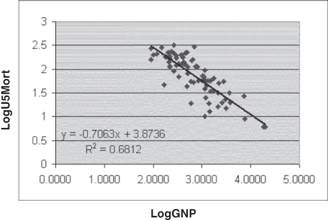
Figure 13.33 Best-fitting line for LogGNP and LogU5Mort: Linear model
Other Trendline Options in Excel
Now that we have introduced the capabilities of the Format Trendline dialog box, it is necessary to say a little about each of the other trendline options. The Logarithmic option produces a curve that is based on conversion of the x-axis variable (GNP, in this case) to its natural logarithm. Ordinary least squares are then performed to generate the regression coefficients and R square. In turn, the resulting predicted values are graphed on the chart with the actual values of GNP. This produces the curve, the regression equation, and the R square shown in Figure 13.34 (see p. XX).

Figure 13.34 Best-fitting line for GNP and U5Mort: Logarithmic model
It is useful to note that the regression constant of 438.09 and the R square of 0.5386 are the same, as they were generated for the relationship shown in Figure 13.27 and detailed in row 9 of Figure 13.15. The only difference is between the equation shown in Figure 13.34, and that indicated in row 9 of Figure 13.15. The value of the coefficient on LogGNP is −116.56 rather than −50.52.
The reason for this difference is that the data used to generate the values in Figure 13.15 were the log of GNP to the base 10. Excel uses the natural logarithm (base 2.71828) for the regression equation shown in Figure 13.34. However, there is a constant relationship between the log to the base 10 and the natural log. Therefore, the coefficient of logGNP in Figure 13.15 can be generated from the coefficient in Figure 13.34 by multiplying by the constant value 2.30585. Thus, the logarithmic model in the Format Trendline dialog box is simply the model generated by taking the log of the independent variable and relating it—using ordinary least squares regression—to the actual value of the dependent variable.
The Polynomial Option in Excel
The fourth option in the Format Trendline window is the Polynomial option. If the Polynomial option is selected, it is possible to select 2 through 6 from the scroll arrows beside the Polynomial option. If you select 2, you produce a second-degree curve with one change of direction. Selecting 3 produces a third-degree curve with two changes of direction, and so on. Selection of 2 produces exactly the same result in terms of predicted values and the same regression equation and R square as were produced for Figure 13.26 and given in Equation 13.7. If the Polynomial option is selected, it is important to realize that there will be as many predictors in the model as the number selected plus a constant. In other words, if 2 is selected, the model will contain the x-axis variable plus its square and a constant. If 3 is selected, the model will contain the x-axis variable plus its square, its cube, and a constant, and so on.
The Power Option in Excel
The fifth option available in the Format Trendline dialog box is the Power option, the result of which is shown in Figure 13.35. The equation for the Power option, given in the figure, is the most complex yet encountered. But look at the R square for the power option. At 0.6812, it looks suspiciously like the R square for the model in which both GNP and U5Mort are converted to their log values (Figure 13.33). Furthermore, the 20.7063 power to which x is raised in Figure 13.35 looks very much like the 20.7063 by which x is multiplied in Figure 13.33.

Figure 13.35 Best-fitting line for GNP and U5Mort: Power model
Moreover, if we take the 3.8736 in Figure 13.33 and raise 10 to that power, we get 7,475.5, which is the multiplier of x in Figure 13.35. Thus, the formula for the Power model can be found by using ordinary least squares. First, convert both the independent and dependent variables to their log values (base 10), and calculate the regression coefficients. The next step is to set up an equation in which the actual value of the dependent variable is predicted by using the actual value of the independent variable. This is accomplished by raising the independent variable to the power of the coefficient on the log of the dependent variable and multiplying by 10, then raising it to the power of the intercept. The result is the Power model.
The Exponential Option in Excel
The first option in the Format Trendline dialog box is the Exponential model. The line, equation, and R square for the exponential model are shown in Figure 13.36. The coefficients of the Exponential model can be found, using ordinary least squares, by first converting the dependent variable to its natural logarithm. The next step is to calculate the ordinary least square coefficients. This is accomplished by using the actual value of the independent variable and the natural log of the dependent variable. In the case of the GNP and U5Mort data, this produces the result shown in Equation 13.10. To get the values of U5Mort as expressed in the formula given in Figure 13.36, a few calculations must be completed. First, it is necessary to raise e (2.718282) to the power of the coefficient of GNP shown in Equation 13.10 and 10 times the actual value of GNP. Second, multiply that result by e raised to the power of the intercept term in Equation 13.10. This produces the result shown in Figure 13.36.

Figure 13.36 Best-fitting line for GNP and U5Mort: Exponential model
The last option shown in the Format Trendline dialog box is the Moving Average model. The Moving Average model applies specifically to time-related data, data where there is one measure for each of a string of time intervals. Because this book does not deal with time-related data, the Moving Average model will not be discussed.