Chapter 12
Multiple Regression: Concepts and Calculation
Chapter 11 considered simple linear regression, its calculation, and its interpretation. This chapter extends the simple linear regression model to include more than one predictor variable. This is what is known as multiple regression. This chapter will consider the nature of multiple regression and the calculation of the basic multiple regression results.
Appendix A, “Multiple Regression and Matrices,” discussing the multiple regression and matrix algebra, can be found at the end of the book.
12.1 Introduction
Health care professionals are often faced with the need to describe and analyze relationships between outcomes and predictors. They seek to identify and explain trends, test hypotheses, and/or develop forecasting models. Linear regression models are able to incorporate complex mathematical functions to describe the associations between sets of variables. Given the availability of data in health care administration databases, the application of linear regression can result in improved health care decision making.
In introducing the multiple regression model, we will contrast it to simple linear regression. In this contrast, the Microsoft Excel regression add-in, considered in Chapter 11, will be extended to multiple regression.
Multiple regression analysis is a way for us to understand more about the relationship between several independent or predictor variables and a dependent or criterion variable.
The Extension of Simple Linear Regression
The simple linear regression model is shown in Equation 12.1. In the simple linear regression model, the coefficient b1 represents the slope of the regression line in an xy graph. The coefficient b0 represents the intercept of the regression line, or the value of the dependent variable y when the independent variable x is equal to 0. The symbol e represents the error—the difference between the actual values of y and the predicted values of y.
The multiple regression model extends the simple linear regression model to include more than one independent variable. In the context of the presentation in Equation 12.1, the multiple regression model could be presented as shown in Equation 12.2. In Equation 12.2, the subscript m represents any number of independent variables, and the three dots in a row represent the b coefficients and x variables from 2 to m that are included in the equation but not shown.
The relationship in the simple linear regression model can be envisioned as a line (the regression line) in a two-dimensional graph where, by convention, the horizontal axis is the x variable and the vertical axis is the y variable. This was illustrated in Chapter 11. In simple terms, the relationship of a single independent variable to a dependent variable can be pictured in a two-dimensional space. If there were two independent variables (x variables), it would be possible to picture this relationship as a plane in a three-dimensional space—although this is not easily shown on a two-dimensional medium, such as paper.
If there are more than two independent variables, it becomes impossible to picture this on paper as well. If there are m independent variables, the logical extension is that we should be able to construct a model of all the variables at the same time by producing an m dimensional figure in an m + 1 dimensional space. Although human beings can easily deal with the notion of only three dimensions at a time, it becomes virtually impossible to picture graphically the simultaneous relationship of all x variables to the y variable in m + 1 dimensions. For the purposes of understanding multiple regression, it is not necessary to form this mental picture. We simply need to understand that each independent x variable may have some effect on y that is assessed simultaneously with the effect of all other x variables.
Purpose of Multiple Regression: Dependent and Independent Variable Relationships
The purpose of multiple regression analysis is essentially the same as that of linear regression. We are trying to understand whether there is any relationship between each of the independent variables x and the dependent variable y and in turn what that relationship may be. To do this for simple regression, we learned that two algebraic formulas can be used to find directly the values of b1 and b0.
Similarly, there is a direct algebraic strategy for finding all the coefficients bm and b0 in the multiple regression model. However, the use of this strategy is mathematically complex enough that, until the advent of modern computers, the solution of multiple regression relationships beyond a very few independent variables x was rarely attempted. Fortunately, the Excel add-in that allows us to do simple linear regression easily also allows us to do multiple regression with up to 16 independent variables x. In general, few practical applications of multiple regression require that many independent variables.
To examine the way in which Excel can be used for multiple regression, let us consider the data shown in Figure 12.1. In the figure, the variable y is cost per hospital case for 10 hospitals. The variable X1 is the size of the hospital in number of beds. The variable X2 is a measure of the extent to which the administrator of the hospital can accurately compare his hospital with other hospitals, in terms of costs. An administrator who has a more accurate view of the competition receives a higher score on the visibility scale.

Figure 12.1 Cost data for 10 hospitals
The data shown in Figure 12.1 are wholly fabricated. However, they were fabricated with the recognition that larger hospitals are frequently thought to have lower case costs than smaller hospitals, and hospitals whose administrators are knowledgeable about the competition are also likely to have lower case costs. Even though these data are for only 10 hypothetical hospitals, they can be used to demonstrate both the regression capability of Excel and the calculation of the regression coefficients.
Multiple Regression Using Excel's Data Analysis Add-In
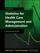
The first step in the description of the use of Excel for multiple regression is a discussion of how the Data Analysis Regression add-in can be used to carry out multiple regression. Recall the initial Regression dialog box, shown in Figure 12.2. This figure also shows the entries needed to produce the regression results. As with simple linear regression, the dependent variable, which is cost, is shown in the Input Y Range field as $B$2:$B$12. The independent variable, however, shown in the Input X Range field, is now different from the simple linear regression model. For multiple regression, the entry for the x variable is given as $C$2:$D$12. Excel has been instructed to select not a single column but two contiguous columns to be included as the independent variable data.
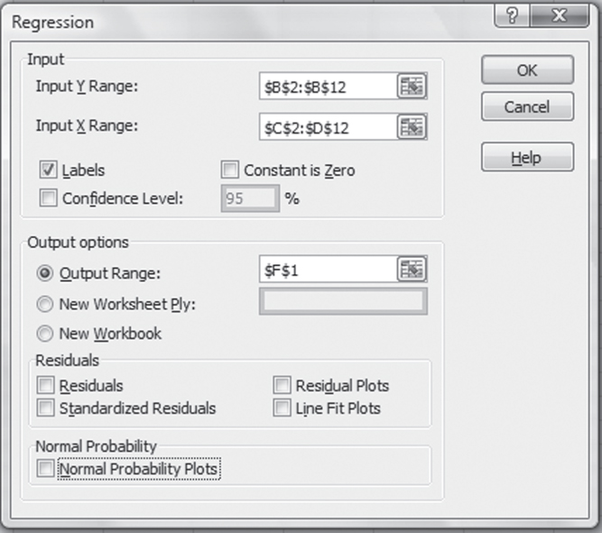
Figure 12.2 Initial Regression dialog box
As was the case with single variable regression, the Labels box has been checked to indicate that the first cell in each row of data is to be treated as a data label. The last important component in the regression window is the output range, which, in this case, is given as cell F1 in the spreadsheet in which the data appear. Clicking OK in this dialog box carries out the multiple regression operation and shows the results beginning in cell F1.
Multiple Linear Regression Using Excel's Data Analysis Package: Step-by-Step Instructions
Follow these step-by-step instructions to invoke the Data Analysis package in Excel and complete the required inputs for linear regression analysis.
- Go to the Data ribbon, in the Analysis group, and click the Data Analysis option.
- A dialog box (Figure 11.8) will appear. Here, choose the Regression option. Another dialog box (Figure 12.2) will appear.
- In the Input Y Range field, enter
$B$2:$B$12or highlight cells B2:B12. - In the Input X Range field, enter
$C$2:$C$12or highlight cells C2:C12. - Click the Output Range radio button, and enter
$F$1. - Click OK, and the Regression output will be created (see Figure 12.3).

Figure 12.3 Multiple regression output
Interpreting the Output from Excel's Multiple Regression Package
The results of the multiple regression are shown in Figure 12.3. This figure is quite similar to that for simple linear regression. However, instead of having one named variable (other than the intercept), there are two: Size and Visibility. The interpretation of the multiple regression output given in Figure 12.3 is essentially the same as the interpretation for simple linear regression. The interpretation of the Regression Statistics section is essentially the same as that of simple linear regression, except that now the adjusted R square takes into account the two independent variables. The analysis of variance (ANOVA) is interpreted just as it was in simple linear regression, but it should be noted that there are now two degrees of freedom in the regression and n − 3 in the residual. The regression coefficients are also interpreted exactly as in simple linear regression except that there are now two slope coefficients rather than one.
There is an important point to consider when interpreting the slope coefficients: In simple linear regression we saw that the regression line could be graphed quite clearly as a straight line in a two-dimensional space. In other words, the graph is two-dimensional with the x or independent variable on the horizontal axis and the y or dependent variable on the vertical axis. With two independent variables, a graph of the predicted values would have to be a plane (a two-dimensional figure) in a three-dimensional space.
By extension, if we were to hope to graph the results of, for example, five independent variables, a five-dimensional figure in a six-dimensional space would have to be created. Because the average human being cannot generate a mental image of any space with more than three dimensions, it should be apparent that it would be impossible to produce a visual image of the results of most multiple regression analyses. In short, the useful visual aids are pretty much limited to simple linear regression.
There is another point to clarify when looking at the coefficients from multiple regression: These coefficients are computed simultaneously. If either coefficient were calculated independently (i.e., in a simple linear regression), it would not be equal to the coefficients calculated in multiple regression. This point is true except in that unusual situation in which there is absolutely no relationship between the two independent variables. Furthermore, the R square obtained from multiple regression is not the sum of the R square that would be obtained from two simple linear regressions with the same two variables. In fact, either of the two independent variables may produce nearly as large an R square as the two variables taken together.
- Multiple R Multiple R represents the strength of the linear relationship between the actual and the estimated values for the dependent variables. The scale ranges from –1.0 to 1.0, where 1.0 indicates a good direct relationship and –1 indicates a good inverse relationship.
- R Square R2 is a symbol for a coefficient of multiple determination between a dependent variable and the independent variables. It tells how much of the variability in the dependent variable is explained by the independent variables. R2 is a goodness-of-fit measure, and the scale ranges from 0.0 to 1.0.
- Adjusted R Square In the adjusted R square, R2 is adjusted to give a truer estimate of how much the independent variables in a regression analysis explain the dependent variable. Taking into account the number of independent variables makes the adjustment.
- Standard Error of Estimates
The standard error of estimates is a regression line. The error is how much the research is off when the regression line is used to predict particular scores. The standard error is the standard deviation of those errors from the regression line. The standard error of estimate is thus a measure of the variability of the errors. It measures the average error over the entire scatter plot.
The lower the standard error of estimate, the higher the degree of linear relationship between the two variables in the regression. The larger the standard error, the less confidence can be put in the estimate.
- t Statistic
The rule of thumb says the absolute value of t should be greater than 2. To be more accurate, the t table has been used.
The critical values can be found in the back of most statistical textbooks. The critical value is the value that determines the critical regions in a sampling distribution. The critical values separate the obtained values that will and will not result in rejecting the null hypothesis.
- F Statistic
The F statistic is a broad picture statistic that intends to test the efficacy of the entire regression model presented.
A hypothesis is tested that looks at H0: B1 = B2 = 0. If this hypothesis is rejected, this implies that the explanatory variables in the regression equation being proposed are doing a good job of explaining the variation in the dependent variable Y.
The Solution to the Multiple Regression Problem
In Chapter 11, we learned how to calculate the regression coefficients from original data and found that the results we obtained were exactly the same as those obtained by the Excel Data Analysis Regression package. In this chapter we are going to look at how the results of multiple regression can be found. In general, because the multiple regression coefficients are found simultaneously, the formula for the solution of the multiple regression problem is not as easily expressed as the solution for the simple linear regression.
This section examines the case of two independent variables as the simplest multiple regression case. Also, this section introduces the use of some relatively elementary calculus. You do not need to understand the calculus involved to use the results or do anything else in this book. However, those who do understand calculus should be able to see how it is possible to arrive at the equations necessary to solve the multiple regression problems. Recall that the criterion for a best-fitting regression result is as that shown in Equation 12.3. If there are two independent variables, as discussed earlier in Section 12.1, then Equation 12.3 can be defined as shown in Equation 12.4, where b0 represents the coefficient for the intercept.
If ![]() is as given in Equation 12.4, then the problem of multiple regression is to find the coefficients bj that minimize the expression in Equation 12.5.
is as given in Equation 12.4, then the problem of multiple regression is to find the coefficients bj that minimize the expression in Equation 12.5.
The Calculus behind the Formulas
Calculus provides a direct solution to the problem of finding the formulas that provide the coefficients bj that minimize the expression in Equation 12.5. The solution is to take the partial derivative of Equation 12.5, with respect to each of the three bj coefficients. Although how this is done may not be clear to you if you don't understand calculus, don't despair. It is important to know only that it can be done; you will never have to know how to do it in order to understand anything else in this section of the book—or in the book in general.
Using calculus, the partial derivative of Equation 12.5 is found, with respect to each of the three bj coefficients. The result will be three new equations, as shown in Equation 12.6.

It is the case that if we set the equations in Equation 12.6 equal to 0, we can solve for the regression coefficients that will best fit the original dependent variable data. After setting the three equations equal to 0, we can drop the partial derivative signs in the equations (the symbols in front of the equal signs). After a little algebra, we end up with the three formulations in Equation 12.7.

or

Solving the Simultaneous Equations Using Excel
Equation 12.7 represents a set of simultaneous equations. Because both the independent variables denoted by x and the dependent variable y are known values, all of the terms in Equation 12.7 that involve summations of x or y can be calculated. Hence, they are known values. But the coefficients bj are what we are interested in discovering. They are the unknown values. With that in mind, you might recognize the second three expressions in Equation 12.7 as being three equations with three unknowns. In general, a set of equations with an equal number of unknowns can be solved simultaneously for the unknown values. Thus, we should be able to solve this set of three equations for the coefficients bj that we wish to find. If you remember high school algebra, you know that you can solve this problem with successive elimination.
Calculating the X and Y Summations
The first step in the successive elimination process is to find the various summations involving x and y. Figure 12.4 shows the calculation of the various known values required by the simultaneous equations in Equation 12.7 for our data. The data were originally given in Figure 12.1 and are repeated here. The values in cells G6:G11 were found by using the =SUMPRODUCT() function, which multiplies two separate strings of data together and sums the result of all the multiplication operations. The construction of the =SUMPRODUCT() statement can be seen in the formula line in Figure 12.4 for the variables X1 (Size) and X2 (Visibility).
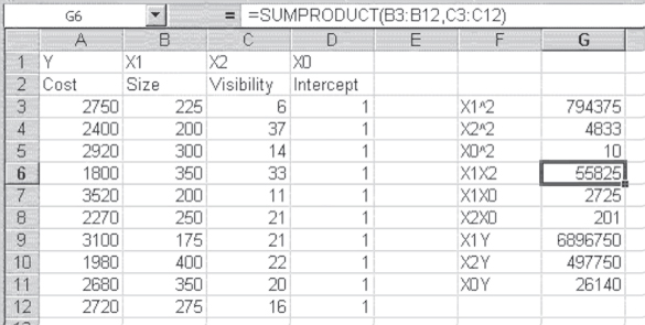
Figure 12.4 Calculation of sums
You can also see in the formula line that the =SUMPRODUCT() function takes two arguments: the data range for the first variable and the data range for the second variable. The values in cells G3:G5 could also have been produced by using the =SUMPRODUCT() function, with the same range entered for each argument. But they were actually produced by using the =SUMSQ() function, which takes one argument and acts by squaring each subsequent value and putting the sum of those operations into the appropriate cell. Table 12.1 displays the formulas for the calculation of sums in Figure 12.4.
Table 12.1 Formulas for Figure 12.4
| Cell or Column | Formula |
| G3 | =SUMSQ(B3:B12) |
| G4 | =SUMSQ(C3:C12) |
| G5 | =SUMSQ(D3:D12) |
| G6 | =SUMPRODUCT(B3:B12,C3:C12) |
| G7 | =SUMPRODUCT(B3:B12,D3:D12) |
| G8 | =SUMPRODUCT(C3:C12,D3:D12) |
| G9 | =SUMPRODUCT(A3:A12,B3:B12) |
| G10 | =SUMPRODUCT(A3:A12,C3:C12) |
| G11 | =SUMPRODUCT(A3:A12,D3:D12) |
Solving for the Coefficients: Successive Elimination
With the various sums calculated that are called for in the three simultaneous equations given in Equation 12.7, it is possible to undertake the solution to the equations. The solution for coefficient bj is shown in Figure 12.5. Rows 15 to 17 in Figure 12.5 represent the three simultaneous equations. The b0, b1, and b2 designations in row 14 represent the coefficient by which each of the numbers in the corresponding row must be multiplied to produce the values in column E, which represent the sums of X1Y, X2Y, and X0Y, respectively.

Figure 12.5 Successive elimination for bj
Successive elimination for the solution of bj proceeds by eliminating, successively, each of the other two coefficients. This is equivalent to finding the value of the equations when the values by which the other coefficients are multiplied are equal to 0. Rows 19, 20, and 21 show the result of finding an equation with two variables and two unknowns with b0 eliminated. Row 15 is replicated in row 19. To produce row 20, row 16 is multiplied by the value in cell A20, which is found by dividing cell D15's value by cell D16's value.
You will note that the result in cell D20 is exactly the value in cell D19. Row 20 is then subtracted from row 19 to produce row 21, which is essentially one equation with two rather than three unknown values, b1 and b2. The same process is repeated in rows 23 to 25. Row 15 is again copied to row 23, but now, to produce row 24, row 17 is multiplied by the value in cell A24, which is cell D15 divided by cell D17. Again, the result in cell D23 is the same as that in D24. Subtracting row 24 from row 23 produces a second equation with two unknowns in row 25.
The final step of this successive elimination is shown in rows 27 to 29. Row 21, the first of the two equations in two unknowns that were found, is copied to row 27. Row 28 is the result of multiplying row 25 by the value in cell A28, which is cell C21 divided by cell C25. Again, note that the values in cells C27 and C28 are equal. Now, subtraction of row 28 from row 27 leaves a single variable (b1) with a nonzero value. The solution to the equation in row 29 is shown in cell B30. You can confirm that that is the same value that was found for the coefficient of Size in Figure 12.3, the Excel Data Analysis ⇨ Regression–produced result.
The other two coefficients can be found in much the same way. It should be clear that successive elimination is a tedious process involving a lot of division, multiplication, and subtraction. Because it is also what is known as an iterative process, it can be very difficult to set up in a systematic way on a spreadsheet. Moreover, as the number of coefficients gets larger, the amount of work involved in the successive elimination approach to solving simultaneous equations grows geometrically. Basically, it is not a very efficient way to do multiple regression. Fortunately, there is a much more efficient way to solve simultaneous equations—essentially to solve the multiple regression problem—and Excel can deal with it quite effectively. But to understand that strategy for finding multiple regression coefficients, it is necessary to understand a little about matrix math, which is the topic of Appendix A that accompanies Chapter 12 (see p. 481).