Chapter 2
Excel as a Statistical Tool
Many people have used Microsoft Excel spreadsheets for financial management, for budget keeping, or for maintaining lists, but not as a statistical tool. Excel has powerful statistical capabilities, and this book uses these statistical capabilities for examples and for problem sets. But to ensure that the user will have some facility with Excel from the outset, this chapter provides a basic introduction to most of what Excel can and will do as a statistical tool. Readers who are already comfortable with the use of Excel might skip Sections 2.1 and 2.2. However, anyone not currently carrying out statistical applications with Excel is likely to benefit from the material in the later sections of the chapter.
2.1 The Basics
Excel is a spreadsheet application. This means that it is made up of columns that are designated by letters (A through XFD) and of rows that are designated by numbers (1 through 1,048,576). There are 16,384 columns and 1,048,576 rows in Excel 2013. Figure 2.1 shows the initial view of an Excel spreadsheet. The intersection of each row and column (e.g., column C and row 12, designated C12 in Excel) is a cell in which, generally, one piece of information can be stored, viewed, and manipulated. This means that there are potentially more than 16 million data cells available on a single spreadsheet. In practical terms, though, it is unlikely that any statistical application will use all the available space on a single spreadsheet. In fact, it is not clear that Excel would function within a reasonable amount of time if it had to manipulate data in a completely full spreadsheet. However, in the vast majority of statistical applications using Excel, it is likely that only a small fraction of the spreadsheet, probably less than 5 percent, will actually be used.

Figure 2.1 Initial view of an Excel spreadsheet
Spreadsheets as Workbooks
Spreadsheets can be grouped in what Excel calls workbooks. Any actual application might consist of a workbook of several worksheets. For example, one spreadsheet might contain an explanation of the application, a second sheet might contain the data, and a third sheet or additional sheets might contain the statistical analyses conducted using the data. If a large amount of data—say, 2,000 or 3,000 observations—is subjected to analysis using several spreadsheets, the resulting data file may become quite large. For most statistical applications, however, this will not be the case.
As shown in Figure 2.1, the Excel spreadsheet includes a ribbon (called the menu bar in earlier versions of Excel) across the top (with the words Home, Insert, Page Layout, and so on representing task-specific ribbons—click a name to display each ribbon). Three icons that are particularly useful to statistical applications are the icon ∑, the icon fx, and the Charts groups icon. The Home ribbon contains the ∑ icon, the function of which is to automatically provide the sum of the values in a set of contiguous cells. The fx icon resides in the Formulas ribbon and calls up an extensive menu of special Excel functions, including statistical and mathematical functions. The Charts group can be found on the Insert ribbon; it allows the user to create a wide variety of charts from one or a number of data entities.
Carrying Out Mathematical Operations
Excel enables the user to carry out all mathematical operations within cells. In carrying out the operations, Excel can refer to other cells for values needed for the arithmetical operations, or actual values (numbers) can be included in cells. Figure 2.2 shows all the important arithmetical operations that will be considered in this book. Row 2 shows the addition of the numbers 5 and 2. As shown in columns D and E, this can be done in two different ways. The addition can be carried out by referencing the cells B2 and C2, in which the values of 5 and 2, respectively, are found (cell D2) or it can be carried out by simply putting the numbers 5 and 2 into the addition equation (cell E2). It should also be noted that Excel arithmetical operations must always begin with the equal sign (=) in order for Excel to recognize that an arithmetical result is desired. Addition and subtraction use the plus sign (+) and minus sign (−), respectively. Multiplication uses the asterisk (*), which appears above the number eight on most keyboards. Division uses the right-leaning slash (/), which is the last key on the right in the bottom row on most keyboards. Raising a number to a power uses the caret (^), which is found above the number six on most keyboards. (The caret, incidentally, is almost universally called “hat” by statisticians.)

Figure 2.2 Excel arithmetical conventions
2.2 Working and Moving Around in a Spreadsheet
One difficulty faced by most novice users of Excel is not knowing how to move around in a spreadsheet and select specific cell references for operations. A second difficulty most new users face is not knowing how to let Excel do the work. This includes allowing Excel to correct mistakes, allowing Excel to enter formulas in multiple cells, and knowing the easy ways to move data around in a spreadsheet. There is absolutely no substitute for actual hands-on experience in learning what the capabilities of Excel are, but some initial hints should be helpful.
Consider the spreadsheet in Figure 2.3, which shows a small data set of 15 records for people who had used a service—for example, that of an ambulatory clinic. The variables shown are an ID or identifier, age of the patient, number of visits to the clinic, total cost of all clinic visits, and average cost per visit. This section also shows three different types of moves that can easily be made within a data set. Assuming a starting point at cell A2, hold down the Ctrl and Shift keys and press the right arrow to highlight the entire row 2 to the first blank column. This also works with Ctrl+Shift+Down arrow, Ctrl+Shift+Left arrow, and Ctrl+Shift+Up arrow. Again, assuming a starting point in cell A2, hold down Ctrl alone and press the down arrow to move the cursor from cell A2 to the last cell in column A that contains data, cell A16. This also works with Ctrl+Right arrow, Ctrl+Left arrow, and Ctrl+Up arrow. Figure 2.3 illustrates that both the current cell and the one next to it are highlighted. Hold down Shift and press the down arrow to highlight both the initial cell (A2) and cell A3. This, too, works with Shift+Left arrow, Shift+Right arrow, and Shift+Up arrow. These operations can also be combined in virtually any order; for example, from a starting point of cell A2, Ctrl+Shift+Right arrow followed by Shift+Down arrow+Down arrow would highlight cells A2 to E4. Or, as a further example, from a starting point in cell A2, Ctrl+Shift+Right arrow followed by Ctrl+Shift+Down arrow would highlight cells A2 to E16.

Figure 2.3 Moving around a data set
Highlighting Cells
Any contiguous group of cells can be highlighted by left-clicking in any corner cell of the area to be highlighted and dragging the cursor to include all the cells that are to be highlighted. Two shortcuts when highlighting cells can make this task much easier. The first of these is Ctrl+Shift+Arrow (right arrow, left arrow, down arrow, up arrow), which will highlight every cell from the selected cell to the last contiguous cell containing data. For example, Figure 2.4 shows the result of the use of Ctrl+Shift+Right arrow when the cursor starts in cell A5. At this point, it is possible to highlight cells A5 to E16 with the use of Ctrl+Shift+Down arrow. The value of this capability is, perhaps, not evident when the data set consists of only 15 rows and 5 columns. But when the data comprises, for example, 357 rows and 42 columns, it is much easier to use Ctrl+Shift+Arrow to highlight all of a row or all of a column than to drag the cursor to highlight all those cells.

Figure 2.4 Result of Ctrl+Shift+Right arrow
The second shortcut that is useful in highlighting is the ability to highlight an entire row (16,384 cells) or an entire column (1,048,576 cells). Clicking either the letter that represents the column or the number that represents the row will highlight the entire column or the entire row. For example, Figure 2.5 shows only the first 18 rows of column B, but clicking the B at the head of the column has highlighted the entire column, from cell 1 to cell 65,536. It is also useful to know that the entire worksheet can be highlighted at one time by clicking in the empty cell at the top of the row-number column (or to the left of the column-letter column).

Figure 2.5 Highlighting an entire column
Copying a Cell to a Range of Cells
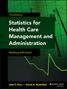
Another useful capability of Excel is its ability to copy one cell to a range of other cells. For example, Figure 2.6 shows the data from Figure 2.3, but before the E column was completely filled in. While the actual spreadsheet from which both Figure 2.3 and Figure 2.6 were taken has numbers in columns A through D (entered manually), cell E2 represents a simple formula (shown in the formula line above the spreadsheet) that simply divides cell D2 (Total Cost) by cell C2 (Visits). The result is the average cost per visit. Rather than typing the same formula in each cell from E3 to E16, or even copying and pasting the formula in each cell, it is possible either to drag or to double-click the formula in cell E2 to all the cells from E3 to E16. To do either, it is necessary to put the cursor on the lower right-hand corner of cell E2, as shown in Figure 2.6. Doing this turns the cursor into a small black cross. With the cursor as a small black cross, dragging with the mouse will copy the formula to each successive cell down the E column. Or, still with the cursor as a small black cross, double-left-clicking with the mouse will fill the entire E column to the last occupied cell in the D column.
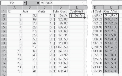
Figure 2.6 Copying a formula to several cells
The double-left-click on the lower left corner can be used to copy a formula down a column as far as the last filled cell in a column on either the right or the left of the column to be filled. But if there is a blank cell on the left of a column, even with a filled column on the right, it is necessary to drag the formula to the end of the data set, because the double-click will go only to the first empty cell on the left. Also, if you wish to copy a formula or other data across columns, or up columns, you can do so only with the drag on the lower right corner of the master cell.
Moving Data with Drag and Drop
Moving data around in Excel is made easy with the use of drag and drop. A highlighted area (see cells B1:B16 in Figure 2.7) can be moved anywhere in the spreadsheet simply by placing the cursor on the highlight outline and dragging it to the spot where it is to be placed. This process is illustrated in Figure 2.7. The highlighted area, cells B1:B16, is moved to cells G1:G16. When the drag and drop is completed, the data will no longer be in cells B1:B16. If a drag and drop is executed, any formulas that either referenced or were referenced by the data when the data was in column B will now reference the data correctly in column G.

Figure 2.7 Moving a data range with drag and drop
Undoing Changes
A very useful tool is the Undo command. Suppose you have a large spreadsheet in which a great amount of data has been entered and on which, perhaps, a number of complex operations have been carried out. Just as you are about to save the entire spreadsheet, you somehow inadvertently erase the whole thing. Is this the appropriate time to slit your wrists? No. You can recover the spreadsheet exactly by going to the Quick Access Toolbar, where you will find an arrow, shown in Figure 2.8, that points to the left or, more intuitively, counterclockwise. Clicking this arrow allows you to back up through a series of up to 16 operations and “undo” them. So if you inadvertently cleared an entire data sheet, you could just click the Undo button and your most recent action—the deletion of the spreadsheet's content—would be reversed.

Figure 2.8 The Undo button
2.3 Excel Functions
Clicking the fx icon in the Formulas ribbon displays the Insert Function dialog box, shown in Figure 2.9. At the top of the dialog box is the Search for a function field, and directly below is the drop-down list from which to select a function by category. When a function is selected (such as the AVERAGE function in Figure 2.9), the bottom of the dialog box shows the name of the selected function and a brief description of what it does. To use a particular function, select it and click OK. Excel will then lead you through a short sequence of steps that designate the cells in which the numbers are found for the calculation for the selected function. As an example, the =AVERAGE() function will produce the average value for a series of numbers contained in several cells.

Figure 2.9 Insert Function dialog box
=AVERAGE() Function
Let's take a look at the working of the =AVERAGE() function. Suppose the spreadsheet contains a column of five numbers in cells B4 through B8 and you wish to calculate the average of those five numbers in cell B9. When you click OK in the Insert Function dialog box (see Figure 2.9), the Function Arguments dialog box, shown in Figure 2.10, will be displayed. Several things about this dialog box, with the =AVERAGE() function already selected, are worth discussing. First, the highlighted field designated Number1 shows the five cells—B4 to B9—that are being averaged. These cells are shown by using the standard Excel convention for designating a set of contiguous cells, which is to display them as B4:B9. To the right of this field is an equal sign and the actual numbers that are in the cells. (If there had been, say, 20 cells being averaged, only the first few would have been displayed.) The field marked Number2 can be ignored in this calculation. Below the areas designated Number1 and Number2 is some additional information. The number 31.4 is the actual value of the average that will be put into cell B9 when the calculation is completed. The absence of a number there means that Excel does not have the information needed from you, the user, to calculate a result. Below the result is a brief statement of what the function actually does. Clicking OK will dismiss the dialog box and put the result of the formula into the selected cell (in this case B9).

Figure 2.10 Function Arguments dialog box
Figure 2.11 shows a portion of the spreadsheet in which the =AVERAGE() function has been employed. The representation is a record of total clinic visits for a single outpatient clinic for a five-day period. The purpose is to determine the average number of persons coming to the clinic over these five days. In cell B9 is shown the actual function being calculated. When you click OK in the Function Arguments dialog box (see Figure 2.10), the function statement is replaced by the value 31.4. The average function being shown in cell B9 is also shown in the line just above the spreadsheet area, to the right of the fx icon. This area is known as the formula line or formula bar. In general, if you wish to know if a value in a particular cell is a number or a formula, click the cell to find the answer in the formula line. If it is a formula, the formula for the cell will be displayed in terms of cell references, as shown in Figure 2.11.

Figure 2.11 Calculation of average
Number of Arguments and Excel Functions
It should be noted that the numbers actually being averaged in cell B9 in Figure 2.11 are represented by cell references within the parentheses following the name of the function. This indication of cell references is called an argument of the function. The =AVERAGE() function takes only one argument: the reference to the cells in which the data to be averaged are found. Other Excel functions may take more than one argument, and some functions—for example, =RAND(), which returns a random number between 0 and 1, and =PI(), which returns the value of pi to 14 decimal positions—take none. If a function takes more than one argument, commas separate the arguments when they are given within the parentheses.
Eighty separate statistical functions are built into Excel. Excel also has several mathematical and trigonometric functions that are useful in doing statistical analyses. It may be helpful to look at the various Excel statistical and math and trig functions (click fx and scroll through the functions in the Select a function window) as a means of getting a preview of what the functions do. It is likely that right now most of them will be obscure, but as you work through this book you will become increasingly familiar with many of the functions.
Direct Input of Excel Function
Functions can be invoked in Excel without using the fx icon. If you know the precise spelling and syntax of the function name, you can type it directly into the cell in which it is to be applied. For example, to enter the =AVERAGE() function directly into a spreadsheet, it is necessary to begin with an equal sign (=). This informs Excel that you are going to enter a formula, and it is why functions are referred to throughout this text by the = prefix. (The same convention holds if you want to carry out any mathematical operation, such as adding the numbers in two cells; the addition command must begin with an equal sign for Excel to recognize the input as a mathematical formula.) The equal sign is followed immediately (no spaces) by AVERAGE (it does not have to be in caps), which is followed by (again, no spaces) a left parenthesis. At this point, you can directly type the cell references in which the numbers to be averaged are found, or you can highlight the cells with your cursor. A right parenthesis completes the formula, and pressing Enter calculates the result of the formula, which appears in the selected cell. If the function name is misspelled or the syntax is incorrect, Excel will let you know by showing #NAME? in the cell where the function was to be calculated.
Contiguous and Noncontiguous Cells
In general, any of the Excel functions will operate on any contiguous set of cells. For some functions, such as the =AVERAGE function already discussed, the =SUM function (activated by clicking the ∑ icon on the Formulas ribbon), and a number of others, the numbers do not have to be in contiguous cells. However, if noncontiguous cells are to be the subject of the operation, it is necessary to use the Excel convention of pressing the Ctrl key before highlighting any second or subsequent set of noncontiguous cells that are part of the operation. For example, take a look at the spreadsheet shown in Figure 2.12. The two columns B and D, representing the clinic visits for the five days of two different weeks, could be summed with the =SUM() command, as shown in the formula line. Entering the actual cell references directly into the cell from the keyboard, rather than highlighting the areas with the help of the Ctrl key, will also produce this result. If the cell references were entered from the keyboard, a comma would be used to separate the two different sets of cell references.

Figure 2.12 Summing two noncontiguous areas
2.4 The =IF() Function
The =IF() function is a particularly useful function that provides a way to make decisions within a spreadsheet. The =IF() function tests a condition and produces one result if the condition is true and a different result if the condition is false. For example, suppose that we have the data shown in Figure 2.13. We have 12 patients identified by the numbers 1 through 12 in column A and the minutes they spend waiting in the emergency room identified in column B. In column C, we want to assign a 1 or a 0, depending on whether each patient spent more or less than the average time patients typically spend waiting. Excel allows us to do this with the =IF() function. Column C in Figure 2.13 already has the values of 1 or 0 assigned, using the =IF() function.
Figure 2.13 Use of the =IF() function
The syntax of the function for cell C2 is shown in the formula line. As you can see there, the =IF() function is written with three arguments. The first of the arguments is the decision. In this case, Excel is asked to decide whether the value in cell B2 is greater than (>) the value in $B$15 (the average for all 12 values in column B). The $ convention is used for cell B15 because we want to compare each of the 12 values in column B to the same value, the average for all 12, which is found only in cell B15 (see Section 2.9). The second argument, always separated from the first by a comma, is a 1, and the third argument, again separated by a comma, is a 0. The =IF() function operates by evaluating the relationship in the first argument. If that relationship is true, it assigns the value of the second argument to the cell in which the function is being invoked. If it is false, the =IF() function assigns the value of the third argument to the cell in which the function is being invoked. The way the function works can be stated as follows: If the value in cell B2 is greater than the value in cell B15, put a 1 in cell C2; otherwise, put a 0 in cell C2. This same function is copied to all cells C2 through C13 and automatically produces the desired results.
Nested =IF() Functions
In the example in Figure 2.13, the =IF() function is used to make only a single decision. Nested =IF() functions can be used to make more complex decisions. For example, instead of assigning a 1 or a 0, depending on whether the waiting time was above or below the average, suppose we wished to determine whether the waiting time was short, long, or medium. For the sake of the example, let us say that a short waiting time is anything under 5 minutes and a long waiting time is anything more than 10 minutes. That would leave any waiting time from 5 to 10 minutes as medium.
Figure 2.14 shows one =IF() function nested within another so that Excel can make both decisions simultaneously. What the decision statement (shown in the formula line for cell C2) does is the following: If the value in cell B2 is greater than 10 (shown now as the actual value of 10, and not as a cell reference), the =IF() function assigns the word “Long” to cell C2. If the value in cell B2 is not greater than 10, a second =IF() function asks if the value in cell B2 is less than 5, and if so, it assigns the word “Short” to cell C2 (which is what it actually assigned). If the value in cell B2 is not less than 5, the =IF statement assigns the word “Medium” to cell C2. Excel will operate on up to 64 nested =IF() statements. It is also useful to mention that the exact way in which the nested =IF() function is developed in Figure 2.14 is not the only possible way such a function could be expressed to assign the appropriate term to each waiting time. An alternative nested =IF() function, such as =IF(B2>5, IF(B2>10, “Long”, “Medium”), “Short”), will produce exactly the same result as produced by the statement actually used in the figure.

Figure 2.14 Nested =IF() functions
Figure 2.14 also shows one additional important point: It is possible to produce a number as the result of a decision or it is possible to produce an alphabetic character (or, for that matter, any printable character). But if the result to be produced is not a number, it must be contained in quotation marks in order for the function to work. The function =IF(B2>10, Long, IF(B2<5, Short, Medium)) would result in an Excel error message, which in this case would be to display #NAME? in the cell in which the function was invoked.
2.5 Excel Graphs
The Excel Charts function is exceedingly valuable for an understanding of how data actually look. This can be useful to gain a better understanding of the data, or for helping to ensure that the data conform to the assumptions of particular statistical operations. You invoke the Charts function by selecting the Insert ribbon and then clicking one of the options in the Charts menu or clicking the small arrow in the bottom right corner of the Charts menu.
Insert Chart Menu in Excel
Figure 2.15 shows the Insert Chart dialog box, about which several things should be noted. For example, there are 11 types of standard charts (shown on the left). Several different chart subtypes within the standard types exist for each of these 11 standard types. These are shown on the right. Highlighting the chart type of interest on the left shows (on the right) the subtype of charts that can be produced within that chart type option. When you have selected the appropriate chart type, click OK.

Figure 2.15 Insert Chart dialog box
Identifying and Formatting Chart Data
To begin the charting process, first highlight (select) the data of interest, and then choose a chart style. When you click OK, the chosen type of chart appears in the active spreadsheet. Figure 2.16 displays a basic bar graph for the clinic visit data. You now have many options to choose from. One of the most important is to identify the data shown in the chart. The data making up this chart are the same data that were used to find the average in Figure 2.11. To identify where the data making up the bar graph are coming from, right-click a bar in the bar graph itself. Once you right-click, a pop-up menu will appear, as shown in Figure 2.17. Choose the Select Data option in the menu, and the Select Data Source dialog box, shown in Figure 2.18, appears.

Figure 2.16 A basic bar graph

Figure 2.17 Excel's chart pop-up menu

Figure 2.18 Select Data Source dialog box
The Select Data Source Dialog Box
The Select Data Source dialog box has four distinct areas. The first area is the Chart data range area, at the top. The Chart data range area identifies where the data for the graph are located. As shown in Figure 2.18, the location is =Sheet1!$A$4:$B$8. Sheet1! identifies the data in the table as coming from sheet number 1 of the workbook. This is useful because not only is it possible to use data from a sheet different from the one that may be active at the time the charting process is begun, but also it is possible to use data from more than a single worksheet. The meaning and use of the dollar signs that appear before both the alphabetic column references and the numerical row references are discussed in detail in Section 2.9.
The second area to take a look at is the Switch Row/Column button, which changes the view of the graph. Currently days are listed in the Horizontal (Category) Axis Labels area (area three of interest) and Series 1 is listed in the Legend Entries (Series) area (area four of interest). When you click the Switch Row/Column button, Excel literally switches what is in the Horizontal (Category) Axis Labels area with what is in the Legend Entries (Series) area. If you click the Switch Row/Column, a chart will appear (see Figure 2.19). As noted earlier, this is a different view of the same data. Figure 2.19 now has all days bunched together under one legend key, literally Week1. This feature is very handy when you wish to cross-view your data from different perspectives (e.g., overall visits by day or overall visits by week).

Figure 2.19 A different view of the same data
Formatting the Finished Graph
You can format a graph in Excel in two main ways. One way is to select the Design ribbon and then choose from the groups in the ribbon depending on what type of modification you wish to make. The Chart Layouts group is most likely the first that you should choose; it allows for various chart layout types and provides a quick and easy method for formatting your graph. The Chart Styles group contains many chart styles to choose from if you are interested in changing colors and/or data point/bar configuration.
Another way to format your graph is by right-clicking the graph itself. After you do so, you'll see the pop-up menu shown in Figure 2.20. This menu contains options that allow you to change the chart type, move the chart, format the chart area, and so on.

Figure 2.20 Chart formatting pop-up menu
What we've discussed so far with respect to graphs is only a beginning. A number of exercises in the book will employ Excel's graph capabilities, and further detail on the use of graphs will be given as specific uses of the graph capability are introduced. Some introductory exercises in creating graphs follow.
2.6 Sorting a String of Data
A very useful Excel capability, especially with regard to sample selection (discussed in detail in Chapter 3), is the ability to sort a data set. The entire data set is going to be sorted on two variables, Sex and Age. The first step is to click the Data label to display the Data ribbon. On the Data ribbon, click the Sort icon to display the Sort dialog box (see Figure 2.21). This is the first step in a data sort. This example will be using the small data set introduced in Figure 2.3 with the addition of a column representing Sex (column C). It should be noted that the cursor has been positioned in cell A2 (see Figure 2.22). It doesn't matter in what cell in the data set the cursor is positioned, but it is important to have it inside the boundaries of the contiguous data set that is to be sorted.

Figure 2.21 Sort dialog box

Figure 2.22 Sort dialog box and data to be sorted
The Sort Dialog Box
When you click the Sort icon, two things happen. The entire data set to be sorted is highlighted, and the Sort dialog box appears (see Figure 2.22). We want to sort the data on Sex and Age. To sort data, we use the first drop-down list in the Sort dialog box, Sort by. The options displayed in the list match our column headers because the option My data has headers, located in the upper right of the Sort dialog box, is checked. When this option is checked, the top row is designated as the header row. If you uncheck the box, you can see that the first row in the spreadsheet is then included in the data.
When we click the drop-down list, we can pick Sex as a column to sort on. However, we also wish to sort on Age, and there isn't another drop-down list from which to choose Age. To create another drop-down list under the Column header, click the Add Level button at the top left of the Sort dialog box. Figure 2.23 displays the Sort dialog box with a Column sort option of Sex and another sort option of Age. It is also possible to sort text values in ascending (A to Z) or descending (Z to A) order and to sort numbers from smallest to largest or largest to smallest. We will leave the defaults, which are A to Z for the Sex variable and Smallest to Largest for the Age variable. You can see these options in the Order drop-down list on the right side of the Sort dialog box. Another drop-down list within the Sort dialog box is that for Sort On. The default for the Sort On drop-down menu is Values, and we will leave the default because we wish to sort on values and not another aspect of the data (e.g., cell color or font color).

Figure 2.23 Sort dialog box with two-column sort options
If we click OK, the data will be sorted by both Sex and Age in that order, and you can see the resulting data set in Figure 2.24. Looking at this figure, you can see that the data are ordered first into those who are female and those who are male, and within these two groupings by age from youngest to oldest.

Figure 2.24 Result of data sort on two variables
2.7 The Data Analysis Pack
Excel comes with a set of statistical analysis tools in addition to the functions available with the fx icon. These are contained in what Excel calls the Analysis Tools. The Analysis Tools menu is found on the Data ribbon and is labeled Data Analysis (see Figure 2.25).

Figure 2.25 Data Analysis option
Installing the Data Analysis Pack
Frequently, the Data Analysis option will not be shown, and if that is the case, it means that the Analysis ToolPak has not been “added in” to your version of Excel. To add the Analysis ToolPak, click the File button (at the upper left) and then click the Excel Options button at the bottom left of the drop-down menu (see Figure 2.26). This brings up the Excel Options dialog box. In the dialog box, click the Add-Ins option on the left to display the available add-ins, as shown on the right in Figure 2.27. In this area click the Manage drop-down list at the bottom of the figure, select Excel Add-Ins from the list (in the figure it is already selected), and click the Go button. The Add-Ins dialog box (Figure 2.28) appears.

Figure 2.26 Excel Options button

Figure 2.27 Excel Options dialog box with add-ins screen displayed

Figure 2.28 Add-Ins dialog box with Analysis ToolPak selected
Two of the items in the Add-Ins window are Analysis ToolPak and Analysis ToolPak—VBA. Once these have been checked and you've dismissed the dialog box by clicking OK, the Data Analysis option will appear on the Data ribbon.
When you click the Data Analysis option, the Data Analysis dialog box appears (see Figure 2.29). Shown in the figure is only a sampling of the 19 different analysis options available through the Analysis ToolPak. Selecting a specific analysis (e.g., Correlation) and clicking OK brings up an analysis window that will be tailored to the particular analysis requested. Specific analyses using the Analysis ToolPak are discussed as we move into the various categories of analysis available through this mechanism (e.g., correlation, ANOVA, regression).

Figure 2.29 Data Analysis dialog box
2.8 Functions That Give Results in More than One Cell
Excel incorporates several functions useful for statistical applications that produce results in more than one cell of the worksheet. One of the most important of these is the =FREQUENCY() function, which can be used to calculate frequency distributions for a set of data according to a set of categories. The =FREQUENCY() function takes two arguments—the data range and the range of categories into which the data are to be counted (called bins by Excel).
The =FREQUENCY() Function
The =FREQUENCY() function has two arguments. These are the DATA range (in this case, B2:B13) and the BIN range (C2:C4) (see Figure 2.30). A comma separates the two ranges. The =FREQUENCY() function accumulates the number of observations that lie at or below the value of the bin but lie above the value of the next lower bin. So the bin values are actually the top of the BIN range. You can confirm that the data range contains three numbers that are 3 or lower, six numbers that are 6 or lower, and four numbers that are 9 or lower.

Figure 2.30 Frequency calculation
In order for the =FREQUENCY() function to work properly, it is necessary first to highlight the entire area into which the resulting frequency distribution will be placed. Then, the =FREQUENCY() function is entered into the first of these cells. The results are obtained by pressing Ctrl+Shift and, while holding those keys down, pressing Enter. If this is not done, the correct results will not be obtained.
The =RAND() Function
Excel also includes a function called =RAND(). The =RAND() function inserts a random number into a single cell or, if desired, into any number of cells. As mentioned earlier, =RAND() has no arguments. It is possible to highlight, for example, 20 cells in four rows and five columns. If the =RAND() function is then used, Ctrl+Shift and then Enter will put a random number between 0 and 1 into each of the 20 cells.
To complete functions in Excel that put results into a single cell, it is necessary only to type the function into the appropriately highlighted cell and press Enter. To complete a function that puts a result into more than one cell, it is necessary, first, to highlight all the cells into which the results are to go, enter the formula according to the convention for that formula, and then simultaneously press Ctrl+Shift and then Enter. If Ctrl+Shift+Enter is not used, the right answer will not be obtained.
Matrix Math Functions
Excel also incorporates several functions with the ability to perform matrix math operations directly in the spreadsheet. Most statistical analyses can be carried out without any reference to matrix math. However, such statistical operations as multiple regression are more easily understood by using matrix math. Three matrix math capabilities of Excel are most useful in statistical applications. These are =MMULT(), which multiplies two matrices together; =MINVERSE(), which inverts a matrix; and =TRANSPOSE(), which changes a vertical range of cells into a horizontal range and vice versa. =MMULT() and =MINVERSE() are found in the Math and Trig function category in the Insert Function dialog box (see Figure 2.9); the =TRANSPOSE() function is found in the Lookup and Reference function category.
The =MMULT() Function
The matrix capabilities of Excel are demonstrated partially in Figure 2.31, which shows an example of matrix multiplication (=MMULT()). On the formula bar it is possible to see that the =MMULT() function is multiplying the matrix in A2:D3 times the matrix in F2:G5. The result, for those who are familiar with matrix math, will be a two-by-two matrix (because matrix 1 has two rows and matrix 2 has two columns). In order to complete a matrix operation with Excel, it is necessary to know the dimensions of the resulting matrix. The area of the resulting matrix is highlighted, and the =MMULT() formula is entered into the upper left-hand cell of the highlighted area. The cell references of the two matrices to be multiplied are then typed within the parentheses, or the cell ranges are highlighted, always with a comma separating them. To complete the matrix multiplication operation, it is necessary to use the convention Ctrl+Shift+Enter.

Figure 2.31 Matrix math example
2.9 The Dollar Sign ($ ) Convention for Cell References
An understanding of the dollar sign ($) convention for handling data in a spreadsheet is critical to the maximum effectiveness of Excel operations. The $ symbol in any particular row or column reference indicates that the row or column designation preceded by the $ symbol is fixed.
Absolute and Relative Cell References
In general, Excel uses what are known as absolute and relative cell references. For example, if you wished to average the clinic visits for Week1 in Figure 2.12 (those in column B), the formula would be =AVERAGE(B4:B8). If this operation were carried out, the result would be the average of the five clinic visit totals for Week1. To get the average for the clinic visit totals for Week2, it is possible to copy the result in B9 and paste it into D9. If this is done, the formula in D9 will read =AVERAGE(D4:D8). This is what is meant by relative cell reference. When a formula is copied from one cell in a spreadsheet to another cell, the cell references change to make the formula refer to the same relative area rather than to the same actual area.
The $ Symbol and Absolute References
A $ symbol before any column or row reference means that the particular row or column is fixed (absolute). If the formula in cell B9 discussed earlier had been =AVERAGE($B4:$B9) and that formula had been copied into cell D9, the result would have been that the formula in D9 would still read =AVERAGE($B4:$B9). The value that appeared in cell D9 would be the average of the number of clinic visits in Week1. For example, suppose you wished to know what proportion of all visits occurred on each day of Week1. There are 157 visits to the clinic in Week1. This is shown in cell B9 of Figure 2.32, which now contains the sum of clinic visits for Week1. Column C shows the percentage of visits that took place in each day.

Figure 2.32 Calculations of percentages
In the formula line, it is also possible to see that the formula for the percentage in cell C4 is calculated as =B4/$B$9. The cell reference to B9 in the formula is absolute. This means that it is possible to copy the formula in cell C4 to each of the cells in C5 through C8, and the proper formula will be calculated for each of the cells in the C column. The numerator, being a relative reference, changes for each cell in the C column, whereas the denominator, which is an absolute reference, remains the same for each cell in the C column. For example, the formula in cell C5 is actually =B5/$B$9. Because the percentage values are always in the C column, it would have been equally feasible to use the formula =B4/B$9 to calculate the first percentage and then to copy that formula to each cell in column C. The results would have been the same.
Absolute References and the F4 Function Key
Rather than go through the somewhat tedious process of putting $ symbols in front of each row and column reference when they are needed, you can use the F4 function key to select $ symbol status. It is possible to toggle through all four possible combinations of $ symbols for any cell reference. For example, if the cell reference B9 is entered into a formula, pressing F4 once will change that cell reference to $B$9. Pressing F4 a second time will change the cell reference to B$9. A third press will change the cell reference to $B9, and a fourth press will change it back to B9. The importance and versatility of the dollar sign convention—and the F4 function key—should become clearer as you proceed through the book.
Table 2.1 displays a glossary of key Excel terms that are used throughout the text. The terms definition and chapter location are included in the table.
Table 2.1 Glossary of Key Excel Terms Used throughout Text
| Excel Term | Definition | Chapter Reference |
#DIV/0! |
Excel error message caused by trying to divide by 0. | 2 |
#NAME? |
Excel error message generally denoting the misspelling of an Excel function name. | 2 |
#NUM! |
Excel error message generally caused by trying to perform an undefined mathematical procedure, such as taking the square root of a negative number, or by requesting a result that exceeds Excel's limits, such as =FACT(171). |
8, 12, 14 |
#VALUE! |
Excel error message generally caused by including a nonnumerical value in a mathematical operation. | 2 |
=AND() |
Excel function that returns the result of two comparisons, TRUE if both comparisons are true and FALSE if either comparison is false. | 7 |
=AVERAGE() |
Excel function that returns the mean of a series of data. | 2, 6 |
=BINOMDIST() |
Excel function that returns the probability for the appearance of any value from a binomial distribution, given the number of trials and the outcome probability for a single trial. | 5 |
=CHIDIST() |
Excel function that returns the probability of a chi-square value, given degrees of freedom. | 8, 10 |
=CHIINV() |
Excel function that returns the chi-square value, given the probability of the chi-square value and degrees of freedom. | 8 |
=CHITEST() |
Excel function that returns the probability of a chi-square value, given the observed and expected values. | 8 |
=COUNT() |
Excel function that returns the number of values in a series of numerical data. | 2 |
=COUNTIF() |
Excel function that returns the number of times a given value appears in a series of data. | 7 |
=EXP() |
Excel function that returns the value of e (approximately 2.718282) raised to the power of the number in the parentheses. | 5 |
=FACT() |
Excel function that returns the factorial of the number in parentheses. Limited to numbers less than 171. | 5 |
=FDIST() |
Excel function that returns the probability of an F value, given degrees of freedom. | 10, 11 |
=FINV() |
Excel function that returns the F value, given the probability of the F value and degrees of freedom. | 10 |
=FREQUENCY() |
Excel function that returns a frequency distribution for a series of data in terms of a series of categories. | 4, 6, 9 |
=IF() |
Excel function that returns the result of an if–then decision. | 2 |
=MAX() |
Excel function that returns the maximum value in a series of data. | 4 |
=MDETERM() |
Excel function that returns the determinant for a square matrix. | 12 |
=MEDIAN() |
Excel function that returns the median value for a series of data. | 6 |
=MIN() |
Excel function that returns the minimum value in a series of data. | 4 |
=MINVERSE() |
Excel function that returns the inverse of a matrix (array). | 12, 14 |
=MMULT() |
Excel function that returns the product of two matrices (arrays). | 2, 12, 14 |
=MODE() |
Excel function that returns the modal value for a series of data. If the data have more than one mode, =MODE() will return the value of the numerically smallest mode. |
6 |
=NORMDIST() |
Excel function that returns probability for any value from a normal distribution, given the mean and standard deviation of the distribution. | 6 |
=OR() |
Excel function that returns TRUE if either or both of two comparisons are true and FALSE if both comparisons are false. | 3 |
=POISSON() |
Excel function that returns the probability of an appearance of any value from a Poisson distribution, given the mean of the distribution. | 5 |
=RAND() |
Excel function that returns a uniform random number between 0 and 1. | 3, 6 |
=RANDBETWEEN() |
Excel function that returns a uniform random number between two selected numbers. | 3 |
=ROUND() |
Excel function that returns the selected number rounded to the number of decimal places specified. | 3 |
=SQRT() |
Excel function that returns the square root of a number. | 6 |
=STDEV() |
Excel function that returns the standard deviation of a series of data assumed to represent a sample. | 6 |
=SUM() |
Excel function that returns the sum of a series of data. | 2 |
=SUMPRODUCT() |
Excel function that returns the sum of the product of the values of two series of data. | 11, 12 |
=SUMSQ() |
Excel function that returns the sum of the squares of a series of data. | 11, 12 |
=TDIST() |
Excel function that returns the probability of a t value, given degrees of freedom and a one- or two-tailed test. | 6, 7, 9, 11, 12 |
=TINV() |
Excel function that returns the t value, given the probability of the t value and degrees of freedom. | 6, 7 |
=TRANSPOSE() |
Excel function that returns the transpose of a matrix (array). | 12, 14 |
=TRUNC() |
Excel function that returns the integer portion of a number. | 3 |
=TTEST() |
Excel function that returns the probability of a t value, given a data set with a numerical dependent variable and a two-level categorical independent variable. | 6, 7 |
|
Excel function that returns the variance of a series of data assumed to represent a sample. | 6 |
=VARP() |
Excel function that returns the variance of a series of data assumed to represent a population. | 6 |
=YEARFRAC |
Excel function that returns the number of years between two calendar dates. | 3 |