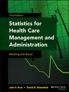
Chapter 14
Analysis with a Dichotomous Categorical Dependent Variable
The chi-square statistic deals with categorical data in both the independent and the dependent variables. However, the general limitation is that only two variables—one independent and one dependent, or, occasionally, two independent and one dependent—can be analyzed at one time. Furthermore, the chi-square is limited by the need to retain relatively large values (at least five or more) in all the cells of the tables in the analysis. The t test and analysis of variance (ANOVA) deal with categorical data in the independent variable but require a numerical variable in the dependent variable. Again, though, t tests are limited to a single independent variable that can take on only two values, whereas ANOVA is usually limited to no more than one or two independent variables. Regression analysis, the topic of the three previous chapters, is more flexible than any of the other three analysis methods. Regression can deal simultaneously with a large number of independent variables, and these can be either numerical or categorical. In addition, regression has no particular cell size requirements. But like t tests and ANOVA, regression as discussed thus far is limited to numerical data in the dependent variable. Frequently, though, there may arise a need to deal with categorical data in the dependent variable, and the desire may be to examine several (or many) independent variables simultaneously. This chapter addresses some alternative approaches to this problem—when the dependent variable is a dichotomous categorical variable.
14.1 Introduction to the Dichotomous Dependent Variable
As has been discussed, a dichotomous categorical variable is one that takes on only two values. Gender, emergency or non-emergency, and Medicare or non-Medicare patients are all examples of dichotomous categorical variables—also referred to as “dummy” variables especially when used as predictor or independent variables in regression analyses. They are universally coded 1 and 0, 1 designating one of the two alternatives and 0 designating the other. But it is also possible to consider a dichotomous categorical variable as a dependent variable. When this is done, the variable is again universally coded 1 or 0 to designate the two levels of the variable.
In early treatments of dichotomous dependent variables, it was common to use ordinary least squares regression. This is essentially what has been presented in the previous three chapters. In this form, regression has commonly been referred to as a linear probability model. This is because the predicted value of the dependent variable, based on the analysis, was considered the probability that an observation would be a 1 or a 0, not whether it actually was a 1 or a 0. As with any other regression model, there is a direct mathematical solution to the problem of finding regression coefficients with dichotomous categorical dependent or dummy variables. But there are also some clear problems with using regression with dummy variables. These problems will be discussed in more detail as we proceed.
In recent years, two things have led to the abandonment of ordinary least squares regression to analyze dummy dependent variables. The first has been the recognition of the problems in using ordinary least squares regression to deal with dummy dependent variables. The second has been the increasing availability of statistics software to carry out complex and time-consuming calculations. Especially because of the latter, there has been a universal shift to what is called maximum likelihood estimators, to derive the relationship between one or more independent variables and a dichotomous dependent variable. Two maximum likelihood estimators have gained the most favor in dealing with dichotomous categorical dependent variables—Logit and Probit. These two estimation procedures produce nearly identical results in practice. Because the Logit approach is substantially less complex, it is discussed in this chapter. But before turning to Logit, we will examine the ways in which dichotomous dependent variables have been analyzed in the past as a way of demonstrating the problems attendant with these treatments.
14.2 An Example with a Dichotomous Dependent Variable: Traditional Treatments
The staff at a well-baby clinic is concerned about the immunization levels of children being treated there. The clinic staff hopes to achieve full immunization levels for all children seen at the clinic. The staff also knows that some mothers are more likely than others to seek full immunization for their children and thus will need little or no push from the clinic. The question before the clinic staff is whether it is possible to predict which mothers are likely not to seek full immunization for their children so that they can concentrate their effort on those women in promoting full immunization.
The clinic staff has also observed that younger mothers, mothers with less education, and mothers with a low socioeconomic status (SES) are less likely to have their children fully immunized. The clinic staff are hopeful that knowing this will allow them to better concentrate their effort on education and the promotion of immunization. They have also observed that if a child is a second, third, or higher-birth-order child, it is more likely that the mother will seek full immunization on her own. The clinic has collected data on 32 mothers who are coming to the clinic. Each of these mothers has a child between one and two years of age. The data available to the health department include the mother's age, her years of formal education, the birth order of the child, and whether the child is fully immunized for one year of age. The data (which are wholly fabricated for this example) are shown in Figure 14.1. As the figure shows, the mothers range in age from 17 to 28 years. They have between 5 and 15 years of formal education, and they have one to six children. Of the children, 21 are fully immunized (those coded 1 in the column labeled Immun); the other 11 children are not fully immunized. The question is whether the clinic can gain any information from these data to help them better target their education efforts about immunization.

Figure 14.1 Data for 32 mothers
A Chi-Square Analysis
One way to approach the problem of deciding where to put education efforts is to use contingency table analysis and the chi-square statistic. Contingency tables and chi-square analysis are well suited to dealing with categorical dependent variables. However, contingency tables and the chi-square statistic approach basically require some observations in every cell. It is really not feasible to use this approach without collapsing the independent variable data—age, education, and parity—into some smaller set of categories. One way to collapse the independent variable data would be simply to split them into high and low at the mean. If we do that, the resulting data for the 32 mothers would be as those shown in Figure 14.2, where a 1 designates a value of the original variable that is greater than the mean and 0 represents a value of the original variable less than the mean. This is referred to as one-zero conversion and is displayed in Figure 14.2.

Figure 14.2 One-zero conversion of data for 32 mothers
The data in Figure 14.2 can be used to generate two-by-two contingency tables and chi-square values. In turn, the immunization status of the child can be determined if it is dependent on any of the three variables: age, education, or parity. The analysis for age is shown in Figure 14.3. That figure shows the pivot table results of crossing immunization with age in cells N3:Q7. In cells N9:Q13, the expected values for the cells in the original pivot table are given.

Figure 14.3 Chi-square analysis of immunization by age of mother
Issues with Chi-Square Analysis
One problem with using chi-square analysis for these data is immediately obvious from either the original data table or the expected value table. That problem is the small cell sizes, especially for the older age–no immunization category. In consequence, the chi-square is computed by using the Yates's correction. The formula for the contribution to the chi-square of cell O17 is shown in the formula bar. Note the absolute value of the difference between the observed and expected values and the 2.5 of the Yates's correction are shown there.
With or without the Yates's correction, the chi-square value produced by the analysis of full immunization by the mother's age suggests that the two variables are statistically independent. The chi-square is given in cell Q21, and its probability is given in cell Q22. Given that the probability of finding a chi-square value as large as 0.539 (if a mother's age and immunization status are independent of one another) is 0.46, we will conclude that they are, in fact, independent. The bottom line is that you can't predict a child's immunization status from the age of its mother.
We can carry out a similar analysis for both a mother's education and the birth order of the child. If we do so, the results are a chi-square of 10.49, with a probability of 0.001 for the mother's education, and a chi-square of 2.24, with a probability of 0.136 for the birth order of the child. The conclusion that we would draw, based on these data, is that of the three things about which the clinic has information, only the mother's education is related to the child's immunization status. Consequently, it would not be unreasonable for clinic staff to conclude that if they hope to have an effect with a targeted information program, they should target women with lower education.
There are a couple of problems with these analyses, though. First, because we have collapsed the data regarding the mother's education and the birth order of the child from multiple levels to just two, we have lost information. It is generally better, if possible, to select an analysis that uses all the available data. Second, we have looked at only one variable at a time. It is also generally better, if possible, to select an analysis that treats all variables of interest simultaneously. Although contingency tables and chi-square analysis can, in certain circumstances, be used to examine more than one independent variable at a time, in this case, the cell sizes would be too small to make it practical.
We have seen in Chapters 12 and 13 that multiple regression uses the full range of data available in the analysis. Multiple regression can also deal simultaneously with a number of independent variables (16 for the Microsoft Excel add-in). Theoretically, the number of independent variables is limited to one fewer than the number of observations. So can we use multiple regression—in this case, ordinary least squares, or OLS—to analyze these data? The answer turns out to be yes and no. To help us see why, the next section discusses the use of OLS with the data on immunization.
Ordinary Least Squares (OLS) with a Dichotomous Dependent Variable
Let us consider the data on children's immunization status, using OLS. Figure 14.4 shows the results of the regression analysis for the data shown in Figure 14.1. The data have been rearranged to carry out the analysis, and only the data for the first 20 women and their children are shown. The results of the analysis, using the Excel regression add-in, are given in cells G1:L20. The analysis indicates that 58 percent of the variance in immunization rates has been accounted for (cell H5). It also indicates a significant overall F test (cells K12 and L12). Furthermore, it confirms the conclusions about the age and education of the mother. Even with the additional data, the age of the mother is not a statistically significant predictor of immunization status (cells H18:K18). The additional data confirm also that a mother's education is a statistically significant predictor of immunization status (cells H19:K19). With the additional data provided by the OLS analysis for birth order of the child, that variable too appears to be a statistically significant predictor of immunization status. So the use of OLS instead of contingency tables and chi-square would lead clinic personnel to conclude that they might effectively concentrate their education effort not only on low-education women but also on low-parity women.

Figure 14.4 Results of OLS for immunization data
Problems with Ordinary Least Squares with a Dichotomous Dependent Variable
But there are also problems with this analysis. The problems have to do with the restriction of the dependent variable to two values: 1 and 0. In this situation the predicted regression values will not be actually 1 or 0. Rather, the values will be some number that must be interpreted as the probability that the true value will be 1 or 0. For this reason, OLS used in this manner is called a linear probability model (LPM). The fact that the actual values of the dependent variable take on only the values of 1 and 0 is not a problem for the regression coefficients themselves. They remain unbiased. The problem lies with the error terms, and thus with statistical tests based on the error terms. A basic assumption of the statistical tests (F tests and t tests) in regression is that the error terms are uncorrelated with the independent variables and have a constant variance and an expected value of 0. Aldrich and Nelson ([1984]) have provided a clear discussion of why these assumptions cannot be maintained when the dependent variable is restricted to 1 and 0. The basic problem is that the variance of the error terms turns out to be correlated systematically with the independent variables. In this situation the statistical tests based on OLS regression are invalid, even in large samples.
But there is a relatively simple fix for this situation in regard to the statistical test, which was originally proposed by Goldberger ([1964]) and clearly laid out by Aldrich and Nelson. This is a weighted least squares (WLS) procedure for estimating the linear probability model.
Weighted Least Squares (WLS) for Estimating Linear Probability Models
The weighted least squares procedure for the linear probability model is carried out in two steps. The first step is to estimate the regression model by using OLS. The second step is to use the results of OLS to create weights by which the original variables—both the independent variables xi and the dependent variable y—are transformed. In turn, estimate the regression model a second time, on the basis of the transformed variables.
The weights for the transformation are as those given in Equation 14.1, which says that a weight for each observation is created by first calculating the predicted values of the dependent variable, using the OLS estimates of the coefficients. Then the predicted value of the dependent variable is multiplied by 1 minus the predicted value, and the square root of that number is taken. Finally, 1 is divided by the resulting value to obtain the appropriate weight. As Aldrich and Nelson point out, this is just the reciprocal of the estimated standard errors of the error term.
Issues with Generating Weights Greater than 1 or Less than 0
There is, however, a basic problem with this procedure for generating weights. Even though the predicted values of the dependent variable are appropriately interpreted as the probability that the dependent variable will be 1 or 0, it is likely that at least some of the predicted values will be either greater than 1 or less than 0. When a number greater than 1 or less than 0 is multiplied by 1 minus itself, it produces a negative result. The square root of a negative number is an imaginary number, and Excel will generate a #NUM! result in the cell that includes the square root of a negative number. Aldrich and Nelson suggest a relatively simple solution to this problem, which is to use some large number less than 1, such as 0.999, in place of the true predicted value when it is greater than 1 and some small number greater than 0, such as 0.001, when the predicted value is less than 0.
Example of Weighted Least Squares Weight Calculation
Figure 14.5 shows the original OLS data for the 32 mothers (only the first 20 are shown), along with the calculation of the weights for WLS. As it is possible to see, the actual OLS regression analysis has been moved to the right and three new columns have been inserted. The first of the new columns (column F) is the predicted value of the dependent variable Immun (which is ![]() in Equation 14.1) and is called Ipred for Immun predicted. The values of Ipred were calculated using the regression formula with the original independent data in columns B, C, and D and the coefficients in cells K17:K21. By inspection of column F, it is possible to see that 3 of the first 20 predicted values of immunization are outside the range 0 to 1. Cells F3, F7, and F18 have values greater than 1, and cell F17 has a value less than 0. To accommodate that problem in the calculation of weights, a new column, Ipredadj—or Immun predicted adjusted—was included as column G. In column G, the Excel
in Equation 14.1) and is called Ipred for Immun predicted. The values of Ipred were calculated using the regression formula with the original independent data in columns B, C, and D and the coefficients in cells K17:K21. By inspection of column F, it is possible to see that 3 of the first 20 predicted values of immunization are outside the range 0 to 1. Cells F3, F7, and F18 have values greater than 1, and cell F17 has a value less than 0. To accommodate that problem in the calculation of weights, a new column, Ipredadj—or Immun predicted adjusted—was included as column G. In column G, the Excel =IF() function is used to adjust the predicted values to ensure that they are all in the range 0 to 1. The =IF() statement as it appears in cell G2, for example, is =IF(F2>1, 0.999, IF(F2<0, 0.001, F2). That =IF() statement is then copied to each cell in column G.

Figure 14.5 Calculation of weights for WLS
The final new column in Figure 14.5 is the actual weight calculated from the adjusted predicted value of Immun. The formula for the calculation of the weights is given, for cell H2, in the formula bar above the spreadsheet. These are the values by which the independent variable set is modified for WLS.
The regression analysis based on the weighted values of the variables is shown in Figure 14.6, which again shows the first 20 mothers in the data set in column A. Column B, labeled Const for constant, is simply the weight calculated in Figure 14.5, but it can be thought of as the constant term in regression (1) multiplied by the weight. Each column—C, D, E, and F—is the original value of each variable—Age, Educ, Order, and Immun—multiplied by the weight from Figure 14.5.

Figure 14.6 Weighted least squares results
Setting Up the Weighted Least Squares Analysis in Excel's Regression Package
The WLS analysis can be carried out on these data by using the regression package in Excel. But it must be employed somewhat differently from the way it is in most regression situations. The WLS procedure requires that each variable, including the dependent variable and the constant term (the value that will determine the intercept), be multiplied by the weight before we proceed with the regression analysis. This means that the variable Const (column B) becomes the set of values that will determine the intercept. In order to carry out the regression analysis with the variable Const as the determinant of the intercept, it is necessary to specify that the intercept is 0 in the regression window.
Recall the Regression analysis dialog box, which is shown again in Figure 14.7. The Input X Range now includes columns B through E. Column B, which represents the intercept term, is now part of the analysis, unlike the previous situations in which Excel was simply assumed to provide the constant for the calculation of the intercept term. At the same time, the box Constant is Zero is now checked. This means that Excel will calculate the regression results without including the column of ones for the intercept. Everything else in the Regression dialog box remains the same.

Figure 14.7 Regression setup for weighted least squares analysis
Interpreting the Output from the Weighted Least Squares Regression
The results of the WLS analysis are shown beginning in column I in Figure 14.6. A major difference between the regression results using OLS (Figure 14.4) and those using WLS is that the place in the regression output where the intercept usually appears (cell J52) is simply a zero, indicating that, in fact, the intercept is being considered 0 by the analysis. The value in cell J53 now represents the intercept term and has the same sign and is of the same order of magnitude as the intercept term in the OLS analysis. Similarly, whereas the other regression coefficients have changed somewhat, these have the same sign and are of the same order of magnitude as the coefficients calculated by using OLS.
The F Statistic
The statistical tests (F and t tests) are now unbiased, but they essentially confirm what was determined by using OLS, which is that both a mother's education level and the birth order of her child, but not the mother's age, influence immunization. On the basis of these results, the clinic might appropriately decide that it should focus education efforts to improve full immunization on women with low education and whose child is low in the birth order.
The R Square Statistic
One thing that might seem somewhat anomalous in the regression output is the magnitude of the R square. In fact, the R square is not meaningful in this case, as it generally is when regression is carried out with a continuous dependent variable. In this case, it represents the proportion of variance in the weighted dependent variable that can be accounted for by the weighted independent variables. But the R square of interest is that which represents the proportion of variance in the original 1, 0 dependent variable that is accounted for by the original independent variables, using the WLS coefficients.
There is some argument about whether an R square with a 1, 0 variable is even meaningful. Let's assume that it is desirable to have some measure comparable to the R square for the WLS analysis. In turn, it is possible to construct a pseudo R square by the formula in Equation 14.2. Equation 14.2 is probably the least conservative (i.e., it will create the largest R square value) of several possible ways in which a pseudo R square might be calculated. The initial step in generating this R square value is to calculate predicted values based on the regression weights given by the WLS analysis, but using the original unweighted data. These predicted values are shown, for the first 20 women, in column G of Figure 14.6. The Excel formula used to create the predicted values is given in the formula bar. Cells B2, C2, and D2 contain the original variables as shown in Figure 14.5. (It should be noted that the original data are in rows 2 through 33.) Now that we have calculated the predicted values based on the original data and the WLS coefficients, it is then possible to calculate error terms for each variable, as shown in Figure 14.8.

Figure 14.8 Calculation of pseudo R square for WLS
Figure 14.8 shows the predicted values of Immun based on the WLS coefficients, as given originally in Figure 14.6, for the first 20 women (column G). Column H shows the error as calculated from the predicted values in column G and the original values of Immun. The equation in the formula bar shows that the first error term is based on the value of Immun in E2, as shown in Figure 14.5. Column I is the square of column H, and the sum of the squared errors (SSE) is given in cell K37. The total of sum of squares (SST) is taken from cell I14 in Figure 14.4 but could be calculated as given in Equation 14.2. The pseudo R square, calculated as (SST−SSE)/SST, is given in cell K39 as 0.518. In general, the pseudo R square calculated this way (or in any other manner) will always be less than the original R square from the OLS analysis.
where ![]() is the familiar
is the familiar ![]() and SSE is
and SSE is ![]() with the values of
with the values of ![]() and
and ![]() being from the original data and
being from the original data and ![]() being the coefficients from the WLS analysis.
being the coefficients from the WLS analysis.
Moving from Weighted Least Squares to Logit Models
Up to this point the WLS results provide a statistically acceptable analysis of the data. The coefficients are unbiased, and the statistical tests are appropriate. But the predicted values of y remain problematic for most serious statisticians. It was mentioned earlier that OLS or WLS employed with a dichotomous dependent variable is referred to as a linear probability model. This is because the predicted values of the dependent variable are essentially equivalent to the probability that the dependent variable will be 1 or 0, depending on the values of the independent variable. All probabilities must be in the range 0 to 1; either a negative probability (less than 0) or a probability greater than 1 is meaningless. But, as can be seen in Figures 14.5 and 14.6, some of the predicted values using either OLS or WLS are greater than 1 or less than 0. The desire on the part of statisticians to remedy this situation in predicting values of dichotomous categorical dependent variables has led to the ascendance of Logit analysis.
14.3 Logit for Estimating Dichotomous Dependent Variables
The previous sections of this chapter have considered chi-square and both ordinary least squares and weighted least squares as ways of dealing with dichotomous dependent variables. This section now takes up the discussion of Logit as a means of analyzing dichotomous dependent variables.
Setting up the Logit Model
The coefficients from a linear probability model, whether calculated using OLS or WLS, will produce a linear relationship between the independent and the dependent variables. If there is only one independent variable x, as well as a dichotomous dependent variable y, the predicted values of the dependent variable (the probabilities of the dependent variable being 0 or 1) will lie along a straight line—for example, as shown by the black diagonal line in Figure 14.9. The diagonal line in Figure 14.9 is actually generated by the linear equation ![]() . The diagonal line could be interpreted as a true probability as long as the value of the independent variable x is between about 5 and 15. If x is less than 5, y is less than 0 and thus cannot be interpreted as a probability. If x is greater than 15, y is greater than 1 and similarly cannot be interpreted as a probability. Because, in general, there is nothing to constrain x to a range from 5 to 15, it would be desirable to be able to specify a relationship—clearly a nonlinear one—that would constrain y to the range 0 to 1 for any values of x.
. The diagonal line could be interpreted as a true probability as long as the value of the independent variable x is between about 5 and 15. If x is less than 5, y is less than 0 and thus cannot be interpreted as a probability. If x is greater than 15, y is greater than 1 and similarly cannot be interpreted as a probability. Because, in general, there is nothing to constrain x to a range from 5 to 15, it would be desirable to be able to specify a relationship—clearly a nonlinear one—that would constrain y to the range 0 to 1 for any values of x.

Figure 14.9 Graph of two relationships between independent and dependent variables
Introduction to Nonlinear Relationships
A number of nonlinear relationships allow the x to vary across any range while confining y to the range 0 to 1. Aldrich and Nelson describe several of these. Of these several alternatives, two have found favor among statisticians—what have come to be called the Logit relationship and the Probit relationship. As the Logit relationship is the simpler of the two, and as they produce almost identical results in the dichotomous dependent variable case, the remainder of this chapter focuses on the Logit relationship.
Introduction to Logit Models
The Logit relationship can be characterized by the gray curved line in Figure 14.9. It might also be called an S curve because it takes on that shape. For the particular Logit relationship pictured, the value of y when x is 10 is 0.5, exactly the same as it is for the linear relationship pictured by the black line. But the Logit relationship approaches both 1 and 0 much more rapidly than does the linear relationship, right to the point where the linear relationship crosses the 1, 0 boundary. When x is 14, for example, the value of y in the linear relationship is 0.86, but for the Logit relationship it is 0.98. However, the Logit relationship never allows the value of y to exceed 1. In fact, it never actually reaches 1 but only approaches it from below. Similarly, the Logit relationship never reaches 0 but only approaches it from above.
The Equation of the Logit Model
The Logit relationship pictured in Figure 14.9 is described by the formula in Equation 14.3. Equation 14.3 says that the values of the probability pi (which represents the predicted values of yi) are given by the value 1 divided by the quantity 1 plus e (approximately 2.718), raised to the power of the regression equation as characterized in OLS or WLS. But the coefficients of the regression equation in Logit are not simply the coefficients derived from OLS or WLS and substituted into the Logit equation. It is necessary to find a whole new set of coefficients to describe the Logit relationship. For example, the actual equation that produced the graph shown in Figure 14.9 was as that shown in Equation 14.4. This can be compared with the equation for the straight line given earlier.
where e is the natural log value of approximately 2.718, and pi is considered to be a probability of any value of yi.
The graph in Figure 14.9 was actually created in Excel. The formula for the Logit relationship as expressed in Excel was =1/(1+ EXP(−(−10+1*x))), where x refers to each value of the independent variable.
Finding the Logit Models Coefficients
If the coefficients for the Logit relationship are not found simply by substituting OLS or WLS coefficients, how then are they found? With OLS and WLS, there is a set of linear equations, derived through calculus, that can be solved to find the regression coefficients directly. With the Logit relationship, there is no such set of equations. The Logit relationship is found by a process known as maximum likelihood. The least squares process, including both OLS and WLS, attempts to minimize the sum of squared error terms through the best selection of coefficients. The maximum likelihood process attempts to maximize the fit between the observed data and a specified model of the data through the best selection of coefficients. The fit is based on the product of all values in the data set times the probability that the values will or will not occur. But products are mathematically difficult to deal with. Therefore, the common solution is to convert the probabilities to logarithms and maximize the fit between the observed data and the log of the specified model. Because of this, the actual value to be maximized in maximum likelihood is referred to as the log-likelihood.
Finding Log-Likelihoods Using Excel
How will this work in the case of Logit and in the specific case of the data on immunization of children? The first step is to set up the relationship for the log-likelihood to be maximized. The log-likelihood function to be maximized is as that given in Equation 14.5. Equation 14.5 is somewhat intimidating, so we will look at the construction of the log-likelihood function to be maximized using Excel.
Figure 14.10 shows the initial step in constructing the log-likelihood function to be maximized. This step is to set up the Logit relationship that defines the probability in Equation 14.3. In column A of Figure 14.10 is shown the identifier for each mother in the study, up to mother 20. Columns B, C, D, and E show the three independent variables—Age, Educ, and Order—and the dependent variable Immun for the first 20 mothers as well. Column F contains the initial calculation of the probability as given in Equation 14.3, and as expressed in Excel. The actual formula for cell F3 is given in the formula bar. In examining the formula for F3 in the formula bar, it is clear that the probability in cell F3 includes the values in cells A1, B1, C1, and D1. These values, 1, 0, 0, and 0, respectively, are initial values of the true coefficients to be found by maximizing the log-likelihood. The first of these, 1, represents the coefficient of the constant. Each of the 0 values represents the coefficient of the variable in the column in which they are located. When the maximization process is finished, these values will have changed to those that maximize logL, as is given in Equation 14.5. It can also be seen that column G contains the value (1 – p), which also enters into the calculation of logL. The Excel formula for cell G3, for example, is simply =1–F3.

Figure 14.10 First step in finding logL
Spreadsheet Layout for Maximizing Log-Likelihoods in Excel
The complete layout for maximizing logL is given in Figure 14.11. Columns A through G remain the same as in Figure 14.10. Column H simply repeats the data in column E but is now designated y to conform to Equation 14.5. Column I is 1 minus column H. Columns J and K represent the calculation of log ![]() and
and ![]() , respectively. The Excel formula for cell J3 is given in the formula bar.
, respectively. The Excel formula for cell J3 is given in the formula bar. =LN is the Excel function for the natural logarithm. Column L is the sum of columns J and K. It should be clear that when y is 1, column L will be log ![]() . When y is 0, column L will be
. When y is 0, column L will be ![]() . There is also a new number, −21, in cell E1. This is the sum of the numbers in column L. It is the log-likelihood, the number to be maximized. It is no accident that the number in E1 is −21. When the coefficient of the constant (cell A1) is 1 and all other coefficients are 0, the log-likelihood for the Logit will always be the negative of the number of ones in the dependent variable. Table 14.1 contains the Excel formulas for Figure 14.11.
. There is also a new number, −21, in cell E1. This is the sum of the numbers in column L. It is the log-likelihood, the number to be maximized. It is no accident that the number in E1 is −21. When the coefficient of the constant (cell A1) is 1 and all other coefficients are 0, the log-likelihood for the Logit will always be the negative of the number of ones in the dependent variable. Table 14.1 contains the Excel formulas for Figure 14.11.

Figure 14.11 Complete layout for maximizing logL
Table 14.1 Formulas for Figure 14.11
| Cell or Column | Formula | Action |
| A1 | 1 | |
| B1 | 0 | |
| C1 | 0 | |
| D1 | 0 | |
| E1 | =SUM(L3:L35) |
|
| F3 | =1/(1+EXP(−($A$1+$ |
Copy down through cell F34 |
B$1*B3+$C$1*C3+$D$1*D3))) |
||
| G3 | =1−F3 |
Copy down through cell G34 |
| H3 | =E3 |
Copy down through cell H34 |
| I3 | =(1−H3) |
Copy down through cell I34 |
| J3 | =LN(F3)*H3 |
Copy down through cell J34 |
| K3 | =LN(G3)*(I3) |
Copy down through cell K34 |
| L3 | =(J3+K3) |
Copy down through cell L34 |
Solving for the Log-Likelihood Coefficients Using Excel's Solver
We have now laid out the spreadsheet for the maximization of the log-likelihood function. How do we find the maximum value of cell E1? Unfortunately, no single set of equations (as with least squares) can be solved for the answer. Basically, the maximization of the log-likelihood function is a trial-and-error process. But there are better and worse methods of going about the process of trial and error to find the set of coefficients that maximize the log-likelihood function. Maddala ([1983]) provides a detailed description of the best process for finding the maximum of the log-likelihood function for the Logit model. However, that discussion is complex enough that for our purposes here, it is bypassed, and we will rely on an add-in capability of Excel to maximize the log-likelihood function.
The Solver Add-In
Excel includes an add-in called Solver. It is accessed within Excel in the same way as the Data Analysis add-in (refer to Chapter 2)—go to the Data ribbon, then to the Analysis menu, and click on Solver (see Figure 2.25). Solver is a general maximization routine that works on a wide variety of applications. In this chapter it is discussed only as it applies to the maximization of the log-likelihood function in Logit.
Setting Up Solver for the Logit Problem
The Solver Parameters dialog box is shown in Figure 14.12. The value to be maximized, in this case, cell E1, is shown in the field next to Set Target Cell. Solver provides several options for what to do with the value in cell E1. It can be maximized, minimized, or set equal to some specified value as determined by the Equal To row. The cells that are to be changed to seek the solution desired (in this case, a maximum) are specified in the field below By Changing Cells. Solver will guess which cells to modify if you wish, and it usually guesses right. Finally, a number of constraints can be set on the solution Solver reaches in the field below Subject to the Constraints. In general, no constraints are required to reach a solution for the Logit model. Click Solve to invoke the add-in after you have made your choices.

Figure 14.12 Solver Parameters dialog box for maximizing logL
The solution to the Logit model arrived at by Solver is shown in Figure 14.13. The value of logL produced by Solver is −6.24 (cell E1). The coefficients of the model that produce this value are given in cells A1:D1. Cell A1 represents the intercept or constant value, and cells B1:D1 represent the coefficients of the three independent variables. Click OK to accept the solution reached by Solver.

Figure 14.13 Solver solution for Logit model
Limitations to Solver when Solving the Logit Problem
There are clear limitations to Solver. The solution reached can depend on the initial values of the coefficients. In general, beginning with the value 1 for the constant and 0 for the independent variables will lead to a solution that represents the best fit between the model and the data. But beginning with other initial values can result in logL's increasing infinitely, so that the result would be a #NUM! in cell E1. If this were to happen, it would be best to begin again with 1 for the intercept and 0 for the other coefficients.
Overall Significance Test with Logit
Having found the coefficients developed by Solver, what is our next step? In least squares regression, one next step would be an overall F test to determine if any of the coefficients of the independent variables are different from 0. With Logit, there is no F test as such, but there is a chi-square test that accomplishes essentially the same thing. The formula for the appropriate chi-square is shown in Equation 14.6. The value of logL1 is given in cell E1 in Figure 14.13. The value of logL0 can be found by recalculating the Solver solution but restricting the cells to be changed (in the By Changing Cells fields; see Figure 14.12) to A1 (the intercept term) only. However, the value of logL0 can also be found, as is given in Equation 14.7. (NOTE: logL is synonymous with LNL that is being used in Equations (14.6) and (14.7).)
where logL0 is the value of logL when all coefficients except the intercept are 0 and logL1 is the value of logL for the best model.
where n is the total sample size, n0 is the number of observations where y equals 0, and n1 is the number of observations where y equals 1.
Figure 14.14 shows the calculation of the chi-square value for the Logit solution shown in Figure 14.13. The value of n, given in cell B1, is 32. The values of n0 and n1, in cells B2 and B3, respectively, are 11 and 21. The value 21.06784 in cell C2 was calculated with the Excel function =LN(B2/B1). Similarly, the value 20.4212 in cell C3 was calculated with the Excel function =LN(B3/B1). L1 in cell B5 was taken from cell E1 in Figure 14.13. Cell B6 was calculated by the Excel statement =B2*C2+B3*C3. The formula for the chi-square value in cell B8 is given in the formula bar. The degrees of freedom for this chi-square are equal to the number of regressors, not counting the intercept, or, in this case, three. The probability of the chi-square value was found with the Excel function =CHIDIST(B8,B9). The chi-square is 28.71 and the p-value is < 0.0001. Therefore, the conclusion of this chi-square test, as with the OLS and WLS F tests, is that at least one of the regression coefficients other than the intercept coefficient is statistically different from 0.

Figure 14.14 Calculation of chi-square for Logit
Significance of Individual Coefficients
Of course, this now leads to the question of how to determine which of the coefficients can be considered different from 0. The test of this is the same as that with OLS or WLS—that is, it is the coefficient divided by its standard error. Unfortunately, though Solver can give us the coefficients, it cannot directly give us the standard errors of those coefficients. To find the standard errors, we must use the coefficients to produce something called the information matrix. The information matrix can most easily be produced using the matrix multiplication capabilities of Excel. To demonstrate the calculation of the information matrix, we must begin with the predicted values of the dependent variable Immun.
Maddala ([1983]) calls the information matrix, based on the best-fit coefficients for the Logit model, ![]() . The standard errors of the coefficients will be the square root of the main diagonal elements in
. The standard errors of the coefficients will be the square root of the main diagonal elements in ![]() , the inverse of the information matrix. To find the information matrix and, hence, its inverse, we need first to find qi for each value of the dependent variable. The value qi can be found as shown in Equation 14.8. The calculation of qi for the data on immunization is shown in Figure 14.15.
, the inverse of the information matrix. To find the information matrix and, hence, its inverse, we need first to find qi for each value of the dependent variable. The value qi can be found as shown in Equation 14.8. The calculation of qi for the data on immunization is shown in Figure 14.15.

where xj includes all regressors and the intercept term.
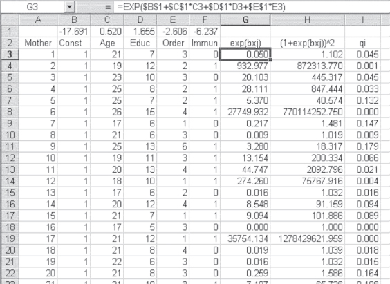
Figure 14.15 First step in the calculation of the information matrix
Calculation of the Information Matrix
Figure 14.15 shows again the data for the first 20 mothers and the coefficients (in row 1) that were generated by Solver in Figure 14.13. A new column has been added as column B, into which has been inserted a column of ones to represent the intercept or constant term. We will use this later in the calculations. All other variables have been shifted one column to the right. Column G is the calculation for the numerator of qi, and column H is the calculation of the denominator. The formula bar shows how cell G3 was calculated. The value qi is shown in column I.
The next step in the calculation of the information matrix is to calculate ![]() for each
for each ![]() , including the intercept term. In the Immunization example, there are three independent variables—Age, Educ, and Order—in addition to the intercept. The construction of the
, including the intercept term. In the Immunization example, there are three independent variables—Age, Educ, and Order—in addition to the intercept. The construction of the ![]() for the intercept and the three independent variables is shown in Figure 14.16. The first five columns in Figure 14.16 are, again, the data for the first 20 mothers. Two columns that appear in Figure 14.15, G and H, have been hidden in Figure 14.16, simply to provide additional room to display the rest of the columns. Column I is
for the intercept and the three independent variables is shown in Figure 14.16. The first five columns in Figure 14.16 are, again, the data for the first 20 mothers. Two columns that appear in Figure 14.15, G and H, have been hidden in Figure 14.16, simply to provide additional room to display the rest of the columns. Column I is ![]() , as calculated in Figure 14.15. Columns J, K, L, and M represent the values of
, as calculated in Figure 14.15. Columns J, K, L, and M represent the values of ![]() , column J being the intercept, which simply repeats the value of qi.
, column J being the intercept, which simply repeats the value of qi.

Figure 14.16 Calculation of qi × xij
Using the =MMULT() and =TRANSPOSE() Functions
The next step in the formation of the information matrix is to prepare to use =MMULT() to multiply the matrix represented by the original data by the transpose of the values in columns J, K, L, and M. To generate the transpose, the best approach is to use the Excel function =TRANSPOSE() and put the result somewhere on the spreadsheet where it will not interfere with other data.
Figure 14.17 shows the first eight columns of the transpose matrix that will be used as the premultiplier for the information matrix. The formula bar shows the =TRANSPOSE() function that was used to create the transpose matrix. The labels were copied from the first row of columns K, J, L, and M to cells V2:V5. If you remember the use of Excel functions that put values into more than one cell (e.g., =FREQUENCY), you remember that the entire area in which the result is to appear must be highlighted before you press Ctrl+Shift+Enter. The easiest way to know exactly what to highlight as the set of target cells for the =TRANSPOSE() function is to use Edit ⇨ Copy to copy the entire original matrix (in this case, cells J3:M34). In turn, in the place where you wish to put the transpose matrix, use Edit ⇨ Paste Special ⇨ Transpose. This will put values into the cells in which you wish the results of =TRANSPOSE() to go. Then you can highlight that entire area and invoke the =TRANSPOSE() function.

Figure 14.17 Formation of the transpose matrix
The information matrix ![]() can now be found by premultiplying the original data matrix (cells B3:E34) by the transpose matrix. Because the transpose is 4 × 32 and the original data matrix is 32 × 4, the resulting information matrix will be 4 × 4. The information matrix, as calculated using the Excel function
can now be found by premultiplying the original data matrix (cells B3:E34) by the transpose matrix. Because the transpose is 4 × 32 and the original data matrix is 32 × 4, the resulting information matrix will be 4 × 4. The information matrix, as calculated using the Excel function =MMULT(), is shown, beginning in cell O3 of Figure 14.18. At this point the reason for adding the column of ones representing the intercept should be clear. It is necessary to include this column in the calculation of the information matrix.

Figure 14.18 Information matrix and t tests
The Standard Errors for the Logit Coefficients
Figure 14.18 also shows the inverse of the information matrix that is calculated using the =MINVERSE function, which begins in cell O9. The standard errors of the Logit coefficients are found by taking the square root of the values on the main diagonal of the inverse of the information matrix. The Logit coefficients themselves are shown in cells O14:R14. The standard errors for each coefficient are shown below them in cells O15:R15. The value in cell O15 (the standard error of the intercept) is the square root of the main diagonal element in the inverse of the information matrix at cell O9. The standard error of the coefficient on Age (cell P15) is the square root of the main diagonal element at cell P10. The standard error of the coefficient on Educ (cell Q15) is the square root of the value in cell Q11. Finally, the standard error of the coefficient for Order (cell R15) is the square root of the value in cell R12.
The t tests are shown in cells O16:R16, and their probabilities are shown in cells O17:R17. The conclusion reached with Logit is exactly the same as that reached with WLS. Both a mother's education level and the birth order of her child influence whether the child is fully immunized, while age does not. So, based on this analysis, if the clinic wishes to increase the proportion of children fully immunized, the staff should concentrate on children whose birth order is low and whose mothers' level of education is low.
Pseudo R Square Statistic
As a final topic in the solution of the Logit problem, it seems reasonable to consider a pseudo R square that can be calculated for the Logit. Aldrich and Nelson suggest as a pseudo R square the value shown in Equation 14.9. Using the formula in Equation 14.9 and the chi-square value from Figure 14.14, the pseudo R square for the Logit analysis is 0.4729. This contrasts with 0.5774 for the OLS analysis and 0.5176 for the WLS analysis.
where X2 is taken from Equation 14.6.
14.4 A Comparison of Ordinary Least Squares, Weighted Least Squares, and Logit
Perhaps the last thing to do in this chapter should be to compare the OLS, WLS, and Logit results in terms of the prediction of whether a child will be fully immunized. How well do these three analyses actually predict which children will be immunized, and how do they compare with one another? The predicted value of the dependent variable Immun is a probability that the true value of Immun will be either 1 or 0; therefore, it seems reasonable to assign a 1 to those observations in which the predicted value of Immun is greater than 0.5 and a 0 to those observations where the predicted value is less than 0.5. (Because none of the predicted values is exactly 0.5, we do not have to worry about what we would do in that case.)
Comparison of the Three Estimates of the Dependent Variable
Figure 14.19 shows a comparison of the three estimates of the dependent variable Immun. The first column in Figure 14.19 represents the mothers in the sample, again, through mother number 20. Column B is the actual value of Immun. Column C is a 1 or 0 value of Immun as predicted by OLS. The =IF statement (as shown in the formula bar) was used to create this as well as columns D and E. Column D is a 1 or 0 value of Immun as predicted by WLS, and column D is a 1 or 0 value as predicted by Logit. Simply looking at the three columns C, D, and E reveals that they are very similar.

Figure 14.19 Comparison of OLS-, WLS-, and Logit-predicted values
Beginning in column G are three pivot tables created from the data in columns B:E. The first pivot table compares the actual values of Immun with the predictions based on OLS. The second compares the actual values with the predictions based on WLS. The third compares the actual values with the predictions based on Logit. For both OLS and Logit, there are two errors. One true 0 is predicted to be a 1, and one true 1 is predicted to be a 0 by both methods. For WLS there are four errors. One true 0 is predicted to be a 1, and the three records that had true values of ‘1’ are predicted to be 0. Though Figure 14.19 does not show this, the match between OLS and Logit predictions is perfect, whereas WLS predicts two observations to be 0, which are predicted to be 1 by OLS and Logit.
It is important to note that this is only one example in a number of comparisons between OLS, WLS, and Logit. However, it appears that OLS and Logit seem to perform about equally in predicting the actual values of a dichotomous dependent variable, and WLS performs slightly less well. In consequence, if the desire is only to predict which observations will be 1 and which will be 0, it seems that OLS, which is relatively simple, compared with Logit, might be satisfactory. However, in this case, OLS did not reveal that birth order was a statistically significant predictor of Immun, whereas both WLS and Logit did. But, in general, if the dependent variable is dichotomous, you cannot go far wrong assuming the Logit relationship and using the techniques described in the Logit section of this chapter.
Note on Interpretation of Logistic Regression Results/Coefficients
Estimated coefficients of a logistic regression model must be interpreted with care. Although the logistic regression coefficients are akin to slope coefficients in a linear regression model their meaning is much different. Slope coefficients in a linear regression model are interpreted as the rate of change in y (the dependent variable) as x's (the independent variables) change. In contrast, the logistic regression coefficient is interpreted as the rate of change in the “log odds” as x changes. This comparison is not very intuitive. However, if we compute the more intuitive “marginal effect” of a continuous independent variable on the probability, the relation is clarified. The marginal effect can be written as:
where f() is the density function of the cumulative probability distribution function (F(BX), which ranges from 0 to 1). In turn, the marginal effects depend on the values of the independent variables. It is often the case that we evaluate the marginal effects of the variables at their means.
The marginal effects can be investigated using the “odds ratio.” The odds ratio is the probability of the event divided by the probability of the nonevent. This interpretation of the logistic coefficient is usually more intuitive where expB is the effect of the independent variable on the “odds ratio.” For example, if ![]() , then a one-unit change in X3 would make the event three times as likely (0.75/0.25) to occur. Odds ratios equal to 1 mean that there is a 50/50 chance that the event will occur with a small change in the independent variable. Negative coefficients lead to odds ratios less than one: if expB2 = 0.5, then a one-unit change in X2 leads to the event being less likely (0.33/0.67) to occur. Just take caution in interpreting negative coefficients as they are harder to interpret than positive coefficients.
, then a one-unit change in X3 would make the event three times as likely (0.75/0.25) to occur. Odds ratios equal to 1 mean that there is a 50/50 chance that the event will occur with a small change in the independent variable. Negative coefficients lead to odds ratios less than one: if expB2 = 0.5, then a one-unit change in X2 leads to the event being less likely (0.33/0.67) to occur. Just take caution in interpreting negative coefficients as they are harder to interpret than positive coefficients.
Survival Analysis: A Brief Discussion
Survival analysis is widely used in health care to quantify “survivorship” in a population being studied. It is termed “survival analysis” because it is indicative of the time elapsed from treatment to death. However, survival analysis is applicable to many areas other than mortality. In short, investigators are concerned with the time from a treatment until an event of interest occurs (i.e., time for a leg fracture to heal after casting).
Survival models can also be viewed as ordinary regression models in which the response variable is time. The three main characteristics of survival models are as follows:
- The dependent variable or response is the waiting time until the occurrence of a well-defined event.
- Observations are censored (i.e., for some units the event of interest has not occurred at the time the data are analyzed).
- Predictors or explanatory variables exist whose effect on waiting time we wish to assess or control.
Table 14.2 juxtaposes the techniques of linear regression, logistic regression, and survival analysis with respect to predictor variables, outcome variable, basic mathematical model, and final model yield.
Table 14.2 Comparing linear regression, logic regression, and survival analysis
| Technique | Predictor Variables | Outcome Variable | Mathematical Model | Yields |
| Linear regression | Categorical or continuous | Normally distributed | Y = B1X + Bo (Linear) | Linear changes |
| Logistic regression | Categorical or continuous | Binary (except in polytomous logistic regression) | Ln(P/1-P) = B1X + Bo (sigmoidal prob.) | Odds ratios |
| Survival analyses | Time and categorical or continuous | Binary | h(t) = ho(t)exp(B1X + Bo) | Hazard rates |
Other reasons survival analysis is preferred to other models are:
- It quantifies time to a single, dichotomous event.
- It handles censored data well.
- It results in a dichotomous (binary) outcome.
- It analyzes the time to an event.
As was previously mentioned, survival analysis is common to health care; however, a more in-depth discussion of the topic is outside the scope of this textbook. Please refer to the following works on survival analysis to obtain a deeper understanding:
- Fleming, T. R., and Harrington, D. P. 2013. Counting Processes and Survival Analysis. Hoboken, NJ: John Wiley & Sons.
- Kleinbaum, D. G. 2011. Survival Analysis: A Self-Learning Text. 3rd ed. New York: Springer.
- Lee, E. T., and Want, J. W. 2013. Statistical Methods for Survival Data Analysis. 4th ed. Hoboken, NJ: John Wiley & Sons.
- Liu, X. 2012. Survival Analysis: Models and Applications. Hoboken, NJ: John Wiley & Sons.