
Appendix A
Multiple Regression and Matrices
In order to understand how the computer carries out regression analysis—which automatically leads to a better understanding of regression—it is necessary to understand something about matrix math. This section provides a brief introduction to matrix math.
Matrices are used to describe linear equations by tracking the coefficients of linear transformations and to record data that depend on multiple parameters.
An Introduction to Matrix Math
A matrix is a set of numbers in a two-dimensional space. Matrices are almost always designated with capital letters in boldface type. In general, a matrix X has n rows and m columns, as shown in Equation A.1, where the first subscript denotes the row and the second denotes the column.

A matrix is said to have dimensions equal to n and m so that the matrix X has dimensions n × m (rows first, columns second). The following is a typical example of a 2 × 3 matrix.
A vector is a matrix with dimensions n × 1 or 1 × m, as shown in Equation A.2.

The following are typical examples of a 3 × 1 vector and a 1 × 3 vector.

A scalar can be considered a matrix of dimensions 1 × 1. The individual entries of any matrix or vector are scalars, but scalars can stand alone. A scalar is simply a number.
The transpose of a matrix X , designated ![]() , is a matrix in which the first row of X becomes the first column of
, is a matrix in which the first row of X becomes the first column of ![]() , the second row of X the second column of
, the second row of X the second column of ![]() , and so on, so that if
, and so on, so that if

or if

Addition and Subtraction of Matrices
Addition and subtraction may be performed on matrices if each has equal rows and equal columns. The two matrices X and Y may be added, as shown in Equation A.3.

The matrix Y can also be subtracted from X, as shown in Equation A.4.

Multiplication of Matrices
Multiplication can be performed on matrices if the number of columns in the first matrix is equal to the number of rows in the second. Such matrices will be said to conform for multiplication. The two matrices ![]() and
and ![]() can be multiplied, and the resulting matrix
can be multiplied, and the resulting matrix ![]() will be of dimension 2 × 2, as shown in Equation A.5. Although
will be of dimension 2 × 2, as shown in Equation A.5. Although ![]() when a and b are both scalars, in general,
when a and b are both scalars, in general, ![]() does not equal
does not equal ![]() and will not have the same dimensions. When the operation
and will not have the same dimensions. When the operation ![]() is carried out, Y may be said to be premultiplied by
is carried out, Y may be said to be premultiplied by ![]() . When
. When ![]() is carried out, Y is postmultiplied by
is carried out, Y is postmultiplied by ![]() . A particularly useful matrix product is
. A particularly useful matrix product is ![]() , which provides the sum of squares and cross products for
, which provides the sum of squares and cross products for ![]() .
.

Matrix Multiplication and Scalars
Any matrices or vectors that are to be multiplied must conform for multiplication, with one exception: Any matrix or vector of any dimension can be pre- or postmultiplied by a scalar, as shown in Equation A.6.

Finding the Determinant of a Matrix
Division is, in general, undefined for matrices. With matrices in which rows equal columns and the determinant of the matrix does not equal 0, multiplication of a matrix by its inverse produces the same result as division. The determinant of a matrix is a scalar defined only for matrices in which rows equal columns. For the 2 × 2 matrix W , the determinant of W may be written as shown in Equation A.7.

If any column of a matrix is a linear transformation of one or more other columns, the determinant will be 0. If, for example, the matrix V is as shown in Equation A.8, the determinant of V will be 0 and the inverse of ![]() will not exist.
will not exist.
In scalar arithmetic, ![]() . If the inverse of a matrix W exists (see Equations A.7 and A.8), then
. If the inverse of a matrix W exists (see Equations A.7 and A.8), then ![]() , where I is a matrix with 1 in each entry on the main diagonal and 0 everywhere else. For example, suppose W is as defined in Equation A.9 (the matrix whose determinant is shown in Equation A.7).
, where I is a matrix with 1 in each entry on the main diagonal and 0 everywhere else. For example, suppose W is as defined in Equation A.9 (the matrix whose determinant is shown in Equation A.7).
Then, W –1 is as defined in Equation A.10, where ![]() , as defined in Equation A.7.
, as defined in Equation A.7.

Finally, ![]() , as shown in Equation A.11.
, as shown in Equation A.11.

Whereas it is relatively easy to find the inverse of a 2 × 2 matrix, finding the inverse of a 3 × 3 or larger matrix becomes increasingly difficult. One method developed early on in linear algebra is the square root method—described, for example, in Harmon (1960). Today it is easier to rely on computer programs that have the capability to produce the matrix inverse in order to obtain it. Fortunately, Excel is one such computer program. In the next section, we look at this capability of Excel's and how it works to solve the simultaneous equation problem of multiple regression.
Matrix Capabilities of Excel
Excel provides several functions that are specifically matrix functions and that are particularly useful in regard to the solution of the multiple regression problem. (Interestingly, Excel refers to matrices as arrays, and that term will be used to refer to a matrix during much of this discussion. But it is often confusing to try to stay with one or the other, so if you see “matrix” and “array” used interchangeably here, just remember that they are basically the same things.) Excel provides four functions that are specifically designed to manipulate arrays (or matrices). These are =MMULT, =MINVERSE, =MDETERM, and =TRANSPOSE.
Excel's Array Functions: =MMULT , =MINVERSE , =MDETERM , and =TRANSPOSE
The first of these functions, =MMULT, multiplies any two arrays together as long as the two conform for multiplication. The second, =MINVERSE, finds the inverse of any square array that has a nonzero determinant. If the determinant of the array is 0, Excel will return NUM# in the cells selected. Excel returns the determinant of the array for =MDETERM and the transpose of the array for =TRANSPOSE. To see how these operate and the results obtained, let us look again at the data in Figure 12.1. We will also use the intercept variable (constant), as shown in Figure 12.4, and this is reproduced in Figure A.1. In Figure A.1, the area that is highlighted in black will be referred to with matrix notation as X (matrices other than those that are m × 1 or 1 × m are always designated with bold roman capitals). The cost column (not highlighted) will be designated with matrix notation as y (matrices that are m × 1 or 1 × m are called vectors and are always referred to with bold roman lowercase letters).

Figure A.1 Hospital data
Manipulating a Matrix with Excel
Figure A.2 shows the data given in Figure A.2, but with several modifications. Now, the independent variable array is designated as simply y , the independent variable array is designated as X , and a new array, designated as X ′, is shown in cells G2:P4. In the formula line in Figure A.2 is the expression {=TRANSPOSE(C2:E11)}. This is the transpose function, and the resulting array X 9 is the transpose of X . It should be noted that the braces surrounding the =TRANSPOSE function mean that it is one of those functions that enter data into more than one cell and must be invoked by holding down Ctrl+Shift and then pressing Enter.

Figure A.2 Arrays y , X , and X′
Using the MMULT Function in Excel
The =MMULT array function can be used to produce two new arrays, X ′X and X ′y, which are shown in Figure A.3. The array X ′X is highlighted, and the formula for that array is shown in the formula bar. It can be seen there that the array is produced with {=MMULT(G2:P4,C2:E11)}. The braces again indicate that the function was completed with Ctrl+Shift+Enter. The array X ′y is produced with the array function {=MMULT(G2:P4,A2:A11)}.

Figure A.3 Arrays X′X and X′y
There is something else to note about Figure A.3 and its comparison with the data in cells G3:G11 of Figure 12.4. The array X ′X includes all the values in cells G3 to G8, and the array X ′y includes the values in cells G9 to G11. The calculation of the X ′X and the X ′y arrays using the matrix capabilities of Excel produces all the values needed for the calculation of the coefficients bj. It is important to note that the results shown in X ′X (3 × 3) would not be the same as the results for X ′X , which would be 10 × 10. Moreover, yX ′ does not even exist, because the two arrays in that format, (10 × 1) and (3 × 10), cannot be multiplied.
Solving the Regression Equations in Excel
Using the data in X ′X and X ′y from Figure A.3, it is possible to rewrite the second three expressions in Equation (12.7), as shown in Equation A.12. We have already seen that these three equations can be solved for the coefficients bj with successive elimination. But with our understanding of matrix math, it can also be seen that Equation A.12 can be rewritten in matrix format, as shown in Equation A.14.


In matrix notation, the formulation in Equation A.14 is ![]() . Now, how can matrix math be used to solve this equation for b? If we were dealing strictly with scalar arithmetic and we had an equation such as
. Now, how can matrix math be used to solve this equation for b? If we were dealing strictly with scalar arithmetic and we had an equation such as ![]() , and x and y were known, we could solve for b by
, and x and y were known, we could solve for b by ![]() . But this formulation is the same as
. But this formulation is the same as ![]() . The expression
. The expression ![]() is the inverse of x and can also be written as
is the inverse of x and can also be written as ![]() . Similarly, in matrix terms, it turns out that if we can find the inverse of
. Similarly, in matrix terms, it turns out that if we can find the inverse of ![]() , we can solve the equation
, we can solve the equation ![]() with the equation X ′X −1 X ′X b = X ′X −1 X y, which turns out to be X ′X −1 X y = b. Happily, Excel provides the ability to find X ′X −1 . To see how Excel provides the inverse, we can look at Figure A.4. In Figure A.4, the inverse of
with the equation X ′X −1 X ′X b = X ′X −1 X y, which turns out to be X ′X −1 X y = b. Happily, Excel provides the ability to find X ′X −1 . To see how Excel provides the inverse, we can look at Figure A.4. In Figure A.4, the inverse of ![]() is shown in the highlighted area, cells M7:O9. The
is shown in the highlighted area, cells M7:O9. The {=MINVERSE()} function used to produce the inverse array is shown on the formula bar. Note again that it is enclosed in braces to denote that it was completed with Ctrl+Shift+Enter. Also, it is important to remember that the entire area consisting of cells M7:O9 was highlighted before the {=MINVERSE()} function was typed.

Figure A.4 Inverse of X′X
Explanation of Excel Output Displayed with Scientific Notation
A further point that should be made about the inverse array is that the numbers, particularly in cells M7, N7, and M8, may appear a little strange. The way these numbers are shown is known as scientific notation. In more familiar terms, the number 1.98E-05 is actually the number 0.0000198. The E-05 means that there are five decimal places before the decimal place in 1.98E-05. It should be recognized that any number that is followed by E with a minus sign and a number is a very small number. Excel uses the E convention to put numbers into cells that otherwise would be two narrow to display the string of decimal places before the actual values begin.
The E convention is also used for very large numbers. For example, a number that would be shown in Excel as 1.98E+11 would actually be 198,000,000,000. This is a relatively economical way for Excel to display very large numbers.
Now that we have found the inverse of ![]() , it is possible to solve for the vector b. This solution is shown in Figure A.5. The coefficients
, it is possible to solve for the vector b. This solution is shown in Figure A.5. The coefficients ![]() (found by the
(found by the =MMULT function, as shown in the formula line of Figure A.5) are exactly the same (except for order and decimal places) as the bj values found by using the built-in Excel package under Data Analysis &cmdarr; Regression. Refer to Figure 12.3 for the Data Analysis results.
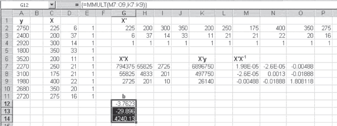
Figure A.5 The b coefficients
Using the b Coefficients to Generate Regression Results
In general, the calculation of all the important results relative to multiple regression can all be developed, once the b coefficients are available. These include the predicted value of ![]() , the total sum of squares
, the total sum of squares ![]() , regression sum of squares
, regression sum of squares ![]() and error sum of squares
and error sum of squares ![]() , the value of
, the value of ![]() and the correlation coefficient (R), the standard error of estimate
and the correlation coefficient (R), the standard error of estimate ![]() , and the F tests. These follow the same development as that described for simple linear regression in Chapter 11. There is one place in which the remaining calculations diverge from that shown for simple linear regression, in the calculation of the standard errors for the coefficients bj. The calculation of the standard errors of the coefficients for multiple regression relies on values that appear only in the matrix X ′X −1 .
, and the F tests. These follow the same development as that described for simple linear regression in Chapter 11. There is one place in which the remaining calculations diverge from that shown for simple linear regression, in the calculation of the standard errors for the coefficients bj. The calculation of the standard errors of the coefficients for multiple regression relies on values that appear only in the matrix X ′X −1 .
Recall that the standard error of estimate, Syx, the standard error of the predicted values of y, is found by dividing the error sum of squares, ![]() , by
, by ![]() and taking the square root of the result. In simple linear regression, the standard error of bj is found by dividing Syx by the square root of the sum of squares in
and taking the square root of the result. In simple linear regression, the standard error of bj is found by dividing Syx by the square root of the sum of squares in ![]() . This is essentially the same as multiplying Syx by the square root of 1/SSX. In multiple regression, the equivalent result is obtained by multiplying Syx by the square root of each of the main diagonal elements of
. This is essentially the same as multiplying Syx by the square root of 1/SSX. In multiple regression, the equivalent result is obtained by multiplying Syx by the square root of each of the main diagonal elements of ![]() .
.
To see the calculation of the standard errors for the coefficients bj, consider Figure A.6. Here the value of Syx has been copied from Figure 12.3. The formula bar shows that the cell highlighted in white is calculated by multiplying the value in cell $M$11 (Syx) by the square root of the value in cell M7 (here 1.98E-05). Because cell $M$11 is fixed, the formula can then be copied into the other cells in row M and in rows N and O to produce, on the main diagonal, the standard errors for all the values of the coefficients b. The expression #NUM! that appears in the off-diagonal cells indicates, in this case, that we tried to take the square root of a negative number. In any case, it is the main diagonal elements that are of interest. It can be seen that except for ordering, they match the values found for the standard errors of the coefficients b in Figure 12.3. These standard error values can be used directly to perform the t test that determines whether the appropriate coefficients are different from 0.

Figure A.6 Calculation of standard errors of b
Calculation of All Multiple Regression Results
Figure A.7 shows the analysis as given in Figure A.5 and Figure A.6. In addition, it shows all the other important results of multiple regression, as shown originally in Figure 12.3. The section of column A labeled ![]() was calculated using the matrix function
was calculated using the matrix function =MMULT(C2:E11,G13:G15), which is essentially the formula for the prediction of the y values cast in matrix form. The values in column C labeled y − ![]() represent the difference between the actual values of y and the mean of y. The value in cell C14 was calculated with the formula
represent the difference between the actual values of y and the mean of y. The value in cell C14 was calculated with the formula =A2–AVERAGE($A$2:$A$11). That formula can be copied all the way to C23 to produce all the y − ![]() values. The value for the total sum of squares, SST, in cell H18, is calculated using the Excel function
values. The value for the total sum of squares, SST, in cell H18, is calculated using the Excel function =SUMSQ(C14:C23).

Figure A.7 Calculation of all results from Figure 12.3
The column labeled yh (for ![]() ) − yb (for
) − yb (for ![]() ) was calculated by subtracting the predicted values of y from the average values for y. The formula for cell D14 is
) was calculated by subtracting the predicted values of y from the average values for y. The formula for cell D14 is =A14–AVERAGE($A$2:$A$11). That formula can be copied to all the cells from D14 to D23 to create all the values of ![]() . The value of the sum of squares due to regression, SSR, in cell H19 is calculated using
. The value of the sum of squares due to regression, SSR, in cell H19 is calculated using =SUMSQ(D14:D23). The column labeled ![]() was calculated by subtracting each value of ŷ from y. The formula for cell E14 is
was calculated by subtracting each value of ŷ from y. The formula for cell E14 is =A2–A14. The sum of squares error, SSE, in cell H20 was calculated using =SUMSQ(E14:E23).
Degrees of freedom in any multiple regression will always be ![]() for SST, equal to m (the number of predictor variables) for SSR, and
for SST, equal to m (the number of predictor variables) for SSR, and ![]() for SSE. In the case of this analysis, these values are shown in cells I18:I20 as 9, 2, and 7, respectively. The mean square values in cells J19 and J20 are the sum of squares values divided by their degrees of freedom. The overall F test for the independence of y from the two variables x is calculated by dividing the mean square due to regression by the mean square error. The probability of the F value, p, is given by the Excel function
for SSE. In the case of this analysis, these values are shown in cells I18:I20 as 9, 2, and 7, respectively. The mean square values in cells J19 and J20 are the sum of squares values divided by their degrees of freedom. The overall F test for the independence of y from the two variables x is calculated by dividing the mean square due to regression by the mean square error. The probability of the F value, p, is given by the Excel function =FDIST(K19,2,7).
The R2 value in cell H22 is calculated by dividing ![]() by
by ![]() . The value of S.E. (standard error of estimate) in cell H23 is obtained by dividing
. The value of S.E. (standard error of estimate) in cell H23 is obtained by dividing ![]() by its degrees of freedom and taking the square root of the result. This value was used to multiply by the square root of the values in cells M12, N13, and 014 to produce the standard error of each value of bj in cells H13:H15. The t values for each of the bj are calculated by dividing each value of b by its standard error. The probabilities of the t values are given by
by its degrees of freedom and taking the square root of the result. This value was used to multiply by the square root of the values in cells M12, N13, and 014 to produce the standard error of each value of bj in cells H13:H15. The t values for each of the bj are calculated by dividing each value of b by its standard error. The probabilities of the t values are given by =TDIST(t,d.f.,2). The degrees of freedom for any value of bj are equal to the degrees of freedom for SSE. Because two of the bj values are negative, the =TDIST function will produce only the result #NUM!. In order to produce the actual probability of the coefficients, it is necessary to include the Excel =ABS function to get the absolute value of t before getting the probability of the t value. So, for example, the probability in cell J13 was obtained with =TDIST(ABS(I13),7,2). Table A.1 displays the formulas for the calculation of the multiple regression output from Figure A.7.
Table A.1 Formulas for Figure A.7
| Cell or Column | Formula | Notes |
| G2:P4 | {=TRANSPOSE(C2:E11)} |
Remember that the braces signify that you must press Crtl+Shift to invoke the function. |
| G7:I9 | {=MMULT(G2:P4,C2:E11)} |
This generates the X × X matrix. |
| K7:K9 | {=MMULT(G2:P4,A2:A11)} |
This generates the X × y matrix. |
| M7:O9 | {=MINVERSE(G7:I9)} |
This generates the X × X−1 matrix. |
| G13:G15 | {=MMULT(M7:O9,K7:K9)} |
This generates the b coefficients. |
| M12 | =323.9537*SQRT(M7) |
Copied from cell M12 through to cell M14 and over to cell O14 |
| A14:A23 | {=MMULT(C2:E11,G13:G15)} |
This generates the ŷ values. |
| C14 | =A2–AVERAGE($A$2:$A$11) |
Copied down to cell C23 |
| D14 | =A14–AVERAGE($A$2:$A$11) |
Copied down to cell D23 |
| E14 | =A2–A14 |
Copied down to cell E23 |
| H18 | =SUMSQ(C14:C23) |
This generates the total sum of squares, SST. |
| H19 | =SUMSQ(D14:D23) |
This generates the sum of square error, SSR. |
| H20 | =SUMSQ(E14:E23) |
This generates the sum of square error, SSE. |
| I18 | 9 | Equals n − 1 or 10 − 1 = 9 |
| I19 | 2 | Equals m or 2 |
| I20 | 7 | Equals n − m − 1 or 10 − 2 − 1=7 |
| J19 | =H19/I19 |
Copied down to cell J20 |
| K19 | =J19/J20 |
|
| L19 | =FDIST(K19,2,7) |
|
| H22 | =H19/H18 |
|
| H23 | =SQRT(H20/I20) |
|
| H13 | =M12 |
|
| H14 | =N13 |
|
| H15 | =O14 |
|
| I13 | =G13/H13 |
Copied down to cell I15 |
| J13 | =TDIST(ABS(I13),I20,I19) |
Copied down to cell J15 |