Appendix E
Optimization Challenge Problems (2‐D and Single OF)
E.1 Introduction
There is a need for convenient test functions for creators to test optimizers and for learners to explore issues. Many that have been offered are simple one‐line functions. Although these can embody certain aspects or features related to optimization, they misrepresent the complexity of real applications and are often contrived idealizations. This collection of test functions seeks to embody first‐principles models of optimization applications to reveal issues, within a step‐better reveal of reality, but remaining relatively simple.
This set of objective functions (OF) was created to provide sample challenges for testing optimizers. The examples are all two‐dimensional, having two decision variables (DVs) so as to provide visual understanding of the issues that they embody. Most are relatively simple to program and compute rather simply, for user convenience. Most represent physically meaningful situations, for the person who wants to see utility and relevance. Most should be understood by those with a STEM degree. All are presented with minimization as the objective.
In all equations that follow, x1 and x2 are the DVs, and f_of_x is the OF value. The DVs are programmed for the range [0, 10]. However, not all functions use DV values in that range. So, the DVs are scaled for the appropriate range and labeled x11 and x22. The OF value f_of_x is similarly scaled for a [0, 10] range. The 0–10 scaling permits a common basis for scaling all functions. It could have been 0–1 or 0–100.
These functions are available in VBA from the Excel file “2‐D Optimization Examples” in www.r3eda.com
E.2 Challenges for Optimizers
Classic challenges to optimizers are objective functions that have
- Non‐quadratic behavior
- Multiple optima
- Stochastic responses
- Asymptotic approach to optima at infinity
- Hard inequality constraints, or infeasible regions
- Slope discontinuities (sharp valleys)
- A gently sagging channel (effectively slope discontinuities)
- Level discontinuities (cliffs)
- Flat spots
- Nearly flat spots
- Very thin global optimum in a large surface (an improbable to find, pinhole optima)
- Discrete, integer, or class DVs mixed with continuous variables
- Underspecified problems with infinite number of equal solutions
- Discontinuous response to seemingly continuous DVs because of discretization in a numerical integration
- Sensitivity of DV or OF solution to givens
Any solution depends on the optimizer algorithm, the coefficients of the algorithm, and the convergence criteria. For instance, a multiplayer optimizer has an increased chance of finding the global optimum. An optimizer based on a quadratic surface assumption (such as successive quadratic or Newton’s) will jump to the optimum when near it, but can jump in the wrong direction when not in the proximity. The values for optimizer coefficients (scaling, switching, number of players, number of replicates, initial step size, tempering, or acceleration) can make an optimizer efficient for one application, but with the same values it might be sluggish or divergent in an application with other features. The convergence criteria may be right for one optimizer but stop another for long before arriving at an optimum. When you are exploring optimizers, realize that the results are dependent on your choice of optimizer coefficients and convergence criteria, as well as the optimizer and the features of the test function.
Metrics for evaluating desirability attributes of optimizers were presented in Chapter 33.
What follows is a description of a variety of 2‐D optimization applications that I believe are useful test applications to reveal a variety of issues. The number that follows the name is the function number in the 2‐D Optimization Examples file.
E.3 Test Functions
E.3.1 Peaks (#30)
This function seems to be a MatLAB creation as a simple representation of several optimization issues. It provides mountains and valleys in the middle of a generally outward sloping surface (Figure E.1). There are two major valleys and, between the three mountains, a small local minima. If the trial solution starts on the north or east side of the mountains, it leads downhill to the north or east boundary. The southern valley has the lowest elevation. The surface is non‐quadratic and has multiple optima.

Figure E.1 Peaks surface.
The function is as follows:
x11 = 3 * (x1 - 5) / 5 'convert my 0-10 DVs to the -3 to +3 range for the functionx22 = 3 * (x2 - 5) / 5f_of_x = 3 * ((1 - x11) ^ 2) * Exp(-1 * x11 ^ 2 - (x22 + 1) ^ 2) - _10 * (x11 / 5 - x11 ^ 3 - x22 ^ 5) * Exp(-1 * x11 ^ 2 - x22 ^ 2) - _(Exp(-1 * (x11 + 1) ^ 2 - x22 ^ 2)) / 3f_of_x = (f_of_x + 6.75) / 1.5 'to convert to a 0 to 10 f_of_x range
E.3.2 Shortest Time (#47)
This simple appearing function is confounding for successive quadratic or Newton’s approaches. It represents a simple situation of a person on sand on one side of a shallow river wanting to minimize the travel time to a point on land on the other side (Figure E.2). It is also kin to light traveling the minimum time path through three media. Variables v1, v3, and v3 are the velocities through the near side, water, and far side; and x1 and x2 represent the E–W distance that the path intersects the near side and far side of the river.

Figure E.2 Shortest‐time path surface.
The VBA code is as follows:
v1 = 1v2 = 0.75v3 = 1.25xa = 1ya = 1xb = 9yb = 9a1 = 3b1 = -0.3a2 = 5b2 = 0.4y1 = a1 + b1 * x1y2 = a2 + b2 * x2distance1 = Sqr((x1 - xa) ^ 2 + (y1 - ya) ^ 2)distance2 = Sqr((x2 - x1) ^ 2 + (y2 - y1) ^ 2)distance3 = Sqr((xb - x2) ^ 2 + (yb - y2) ^ 2)timetravel = distance1 / v1 + distance2 / v2 + distance3 / v3f_of_x = (timetravel - 12) * 10 / (32 - 12)
The problem statement from 2012 was: “She was playing in the sandy area across the river from her house when the dinner bell rang. To get home she needed to run across the sand, run through the shallow lazy river, then run across the field to home. She runs faster on land than on sand. Both are faster than running though the knee‐deep water. What is the shortest‐time path home? On the x‐y space of her world, she starts at location (1, 1) and home is at (9, 9). Perhaps the units are deci‐kilometers (dKm) (tenths of a kilometer). Her speed through water is 0.75 dKm/min, through sand is 1.0 dKm/min, and on land is 1.25 dKm/min. The boundaries of the river are defined by y = 3.0 − 0.3x and y = 5.0 + 0.4x.”
E.3.3 Hose Winder (#46)
This function presents discontinuities to the generally well‐behaved floor. It represents a storage box that winds up a garden hose on a spool (Figure E.3). When the winding hose gets to the end of the spool, it starts back but at a spool diameter that is larger by two‐hose diameters. The diameter jump causes the discontinuities. The objective is to design the storage box size and handle length to minimize the owner’s work in winding the hose.
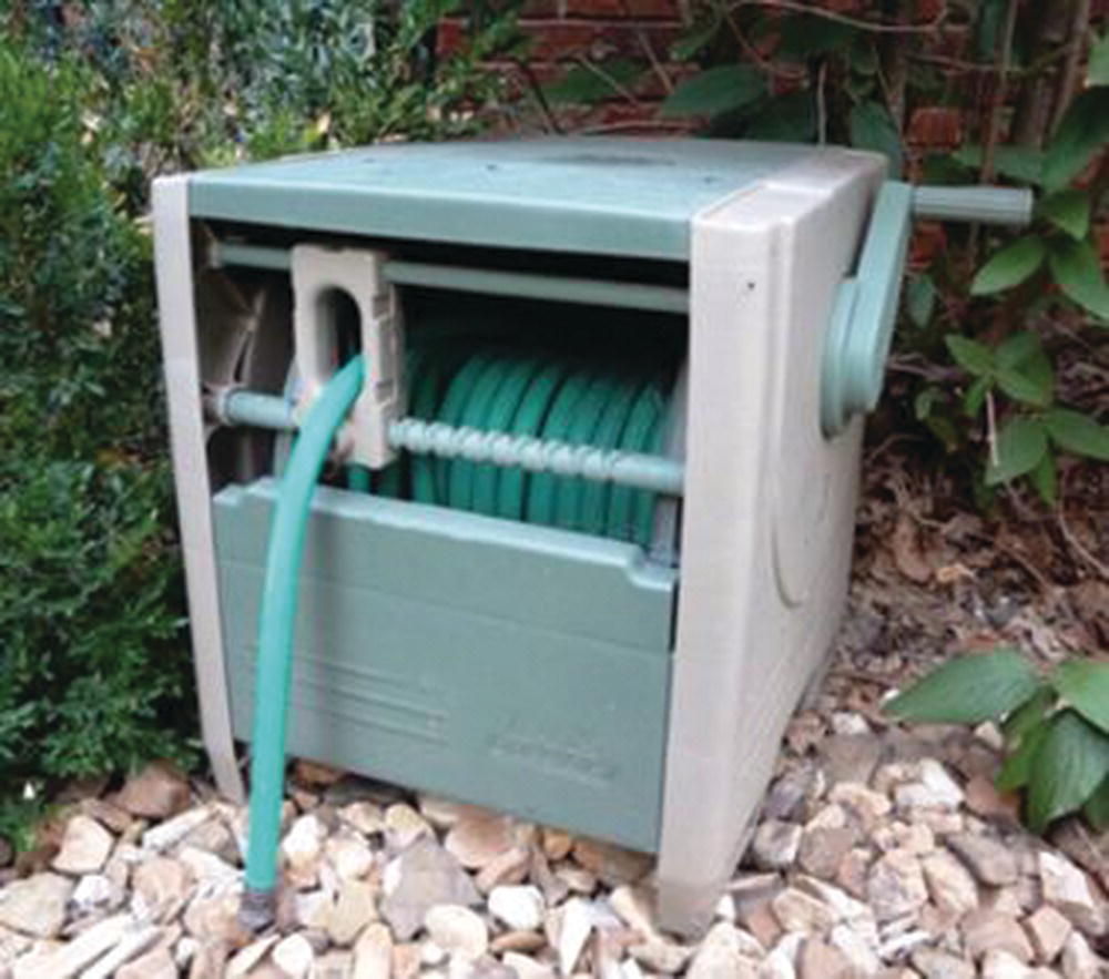
Figure E.3 Hose winder device.
The 2012 problem statement was: “Consider that a hose is 200 feet long, and 1.25 inch in diameter, and is wound on a 6 inch diameter spindle by a gear connection to the handle. The hose goes through a guide, which oscillates side‐to‐side to make the winding uniform. Each sweep of the guide leads to a new hose layer, making the wind‐on diameter 2.5 inches larger.
“Originally the hose is stretched out 200 ft. To reel it in, the human must overcome the drag force of the hose on the ground. Either a smaller spindle diameter or a larger handle radius reduces the handle force required to reel in the hose. As the hose is reeled in, its residual length is less, and the drag force is less. But when the first spindle layer is full and the hose moves to the next layer, the leverage changes, and the windup handle force jumps up.
“After winding 200 ft of hose, the human is exhausted. He had to overcome the internal friction of the device, the hose drag resistance, and move his own body up and down. We wish to design a device that that minimizes the total human work (handle force times distance moving the handle + body work). We also wish to keep the maximum force on the handle less than some excessive value (so that an old man can do the winding). If you increase the handle radius, the force is lessened, but the larger range of motion means more body motion work. There is a constraint on the handle radius—it cannot make the human’s knuckles scrape the ground.
“If you make the spindle length longer, so that more hose is wound on each layer, then the hose wind‐on diameter does not get as large, and the handle needs less force to counter the drag. But more turns to wind‐in the hose means more body motion.
“Further, consider the economics of manufacturing the box. The box volume needs to be large enough to windup the hose on the spindle, and perhaps 20% larger (so that spiders can find space for their webs, it often seems). Use 5 cuft. If the side is square, then defining the length and volume sets the side dimensions. Setting the weight and cost directly proportional to the surface area, the spindle length defines the cost of manufacturing and shipping.
“The objective function is comprised of a penalty for the maximum force, a penalty for the cost, and a penalty for the wind‐up work.”
The 3‐D view indicates a generally smooth approach to a minimum but with local wrinkles on the surface (Figure E.4). The local valleys guide many optimizers to a false minimum.

Figure E.4 Hose winder surface.
The VBA code is as follows:
If x1 <= 0 Or x2 <= 0 Thenconstraint = "FAIL"f_of_x = 15Exit FunctionEnd If' HandleRadius = x1 / 4 'nominal, scales 0-10 to 0-2.5 ft' BoxWidth = x2 / 2 'nominal, scales 0-10 to 0-5 ftHandleRadius = 1.8 + 0.04 * x1 'to focus on discontinuities'BoxWidth = 0.6 + 0.02 * x2 'to focus on discontinuitiesWindRadius = 0.25 'spindle radius 3 inches as 1/4 ftBoxVolume = 5 'cuftBoxSide = Sqr(BoxVolume / BoxWidth)If HandleRadius > 0.85 * BoxSide Thenconstraint = "FAIL"f_of_x = 15Exit FunctionEnd IfArea = 2 * BoxSide ^ 2 + 3 * BoxWidth * BoxSide 'no bottom closureHoseLength = 200 'ftHoseDiameter = 0.1 '1.25 inches = 0.1 ftDragLength = HoseLengthdcircle = 0.025 'fraction of circumfrencework = 0WindLength = 0Fmax = 0Do Until DragLength < 2 'enough increments to wind up hose, leave 2 feet of hose outside winderDragForce = 0.2 * DragLength '0.2 is coefficient of friction lbf/ft of hoseHandleForce = (DragForce * WindRadius + 0.5) / HandleRadius + 1 'hose drag, torque to spin assembly, body motionIf HandleForce > Fmax Then Fmax = HandleForcedwork = HandleForce * HandleRadius * 2 * 3.14159 * dcirclework = work + dworkdlength = WindRadius * 2 * 3.14159 * dcircle 'incremental length wound in one circle incrementWindLength = WindLength + dlength 'total length wound on the layerDragLength = DragLength - dlength 'length of hose left unwooundIf WindLength > (BoxWidth / HoseDiameter) * 2 * 3.14159 * WindRadius Then 'layer full, move to nextWindRadius = WindRadius + HoseDiameter 'update winding radiusWindLength = 0 'reset wound length on new layerEnd IfLoop' f_of_x = 10 * ((Fmax / 5) ^ 2 + (Area / 20) ^ 2 + (work / 1000) ^ 2 - 28) / (70 - 28) 'nominalf_of_x = 10 * ((Fmax / 5) ^ 2 + (Area / 20) ^ 2 + (work / 1000) ^ 2 - 28.25) / (28.45 - 28.25) 'to focus on discontinuities
E.3.4 Boot Print in the Snow (#19)
This represents a water reservoir design problem, but with very simple equations. It is a surrogate deterministic model. The objectives of a reservoir are to trap excessive rain water to prevent downstream floods, to release water downstream to compensate for upstream droughts, and to provide water for human recreational and security needs. We also want to minimize the cost of the dam and land. The questions are how tall should the dam be and how full should the reservoir be kept. The taller it is, the more it costs, but the lower will be the probability of flood or drought impact, and the better the recreational and security features. The fuller it is kept, the less it can absorb floods, but the better the drought or recreational performance. On the other hand, if kept nearly empty, it can mitigate any flood, but cannot provide recreation or drought protection. The contour appears as a boot print in the snow (Figure E.5). The contours represent the economic risk (probability of an event times the cost of the event). The minimum is at the toe. The horizontal axis, x1, represents the dam height. The vertical axis, x2, is the set point portion of full.

Figure E.5 Boot print contour.
A feature of this application that creates difficulty is that the central portion, in the (7, 5) area of the print, is a plane, and optimization algorithms that use a quadratic model (or second derivatives) cannot cope with the zero values of the second derivative.
The VBA code is as follows:
If x1 < 0 Or x2 < 0 Or x1 > 10 Or x2 > 10 Thenconstraint = "FAIL"Exit FunctionEnd Ifx1line = 1 + 0.2 * (x2 - 4) ^ 2deviation = (x1line - x1)penalty = 5 * (1 / (1 + Exp(-3 * deviation))) 'logistic functionalityf_of_x = 0.5 * x1 - 0.2 * x2 + penalty + add_noisef_of_x = 10 * (f_of_x - 0.3) / 6
E.3.5 Boot Print with Pinhole (#21)
This is the same as boot print in the snow, but the global minimum is entered with a small region on the level snow (Figure E.6). Perhaps an acorn fell from a high tree and drilled a hole in the snow. The difficulty is that there is a small probability of starting in the region that would attract the solution to the true global. Nearly everywhere, the trial solution will be attracted to the toe part of the boot print.

Figure E.6 Boot print with pinhole surface.
The VBA code is as follows:
If x1 < 0 Or x2 < 0 Or x1 > 10 Or x2 > 10 Thenconstraint = "FAIL"Exit FunctionEnd Ifx1line = 1 + 0.2 * (x2 - 4) ^ 2deviation = (x1line - x1)penalty = 5 * (1 / (1 + Exp(-3 * deviation))) 'logistic functionalityf_of_x = 0.5 * x1 - 0.2 * x2 + penalty + add_noisex1mc2 = (x1 - 1.5) ^ 2x2mc2 = (x2 - 8.5) ^ 2factor = 1 + (5 * (x1mc2 + x2mc2) - 2) * Exp(-4 * (x1mc2 + x2mc2))f_of_x = factor * f_of_x + add_noisef_of_x = 10 * (f_of_x - 0.3) / 6
E.3.6 Stochastic Boot Print (#20)
This represents the same water reservoir design problem as boot print in the snow; however, the surface is stochastic (Figure E.7). This, too, is a surrogate model. The OF value depends on a probability of the flood or drought event. Because of this each realization of the contour will yield a slightly different appearance. One realization of the 3‐D view is shown. Note that starting in the middle of the DV space on the planar portion, a downhill optimizer will progressively move toward the far side of the illustration where the spikes are. In that region of a small reservoir kept too full or too empty, there is a probability of encountering a costly flood or drought event that the reservoir cannot mitigate. Moving in the downhill direction, the optimizer may, or may not, encounter a costly event. If it does not, it continues to place trial solutions into a region with a high probability of a disastrous event and continues into the bad region as the vagaries of probability generate fortuitous appearing OF values.

Figure E.7 Stochastic boot print surface.
The VBA code is as follows:
If x1 < 0 Or x2 < 0 Or x1 > 10 Or x2 > 10 Thenconstraint = "FAIL"Exit FunctionEnd Ifx1line = 2 + 0.2 * (x2 - 4) ^ 2penalty = 0deviation = (x1line - x1)probability = 1 / (1 + Exp(-1 * deviation)) 'logistic functionalityIf probability > Rnd() Then penalty = 5 * probabilityf_of_x = 0.5 * x1 - 0.2 * x2 + penalty + add_noisef_of_x = 10 * (f_of_x + 1.25) / 7.25
Two realizations of the contour are shown in Figure E.8, which reveals the stochastic nature of the surface, the non‐repeatability of the OF value. Now, in addition to the difficulty of the planar midsection, the optimizer also faces a stochastic surface that could lead to a fortuitous minimum in a high risk section of too small a dam (x‐axis) or keeping the reservoir too full or empty (y‐axis).

Figure E.8 Stochastic boot print contours: (a) one realization and (b) another realization.
E.3.7 Reservoir (#18)
This is the basis for stochastic boot print, but it is a computationally time‐consuming (but not excessively slow) Monte Carlo simulation of a water reservoir. Reservoir capacity and nominal level are the decision variables.
The larger the reservoir, the greater the initial cost. Cost is the objective function. So, superficially, build a small dam and have a small reservoir to reduce cost. However, if the reservoir is too small, and/or it is maintained nearly full, it does not have enough capacity to absorb an upstream flood due to exceptionally heavy rainfall and it will transmit the flood downstream. Downstream flooding incurs a cost of damaged property. But the chance of a flood and the magnitude of the flood depend on the upstream rainfall. So, the simulator models a day‐to‐day status with a lognormal rainfall distribution for a time period of 20 years. (You can change the simulated time or rainfall distribution.)
Contrasting flooding conditions are drought conditions. If the reservoir is too small, and/or maintained with little reserve of water, an upstream drought will require stopping the water release, which stops downstream river flow. Downstream dwellers, recreationists, or water users will not like this. There is also a cost related to zero downstream flow.
There is a fixed cost of the structure and a probabilistic or stochastic cost associated with extreme flood or drought events.
Since one 20‐year simulation will not reveal the confluence of “100‐year events,” the simulator runs 50 reservoirs for 20 years each—50 realizations of the 20‐year period. You can change the number of realizations.
The function is set up to return either the maximum cost for the 50 realizations or the estimated 99% probable upper limit on the cost. You could choose another performance indicator.
An excessively large reservoir kept half full will have ample reserve (to keep water flowing in a drought) and open capacity (to absorb excess rainfall and prevent downstream flooding), but it will cost a lot, both to build and to acquire the land for the lake. A smaller reservoir will have less cost. But too small a reservoir will not prevent problems with drought or flood. So, there is an in‐between optimum size.
If the nominal volume is near the full mark, then the reservoir will not be able to absorb floods, but it will have plenty of capacity for a drought. If the nominal level is too low, it will be able to prevent a flood, but not keep water flowing for a drought event. So, there is also an in‐between set point capacity that is best. The optimum set point for the level might not be at 50%. It depends on whether the vagaries of rainfall and the associated cost impacts make floods a bigger event than droughts.
For any given sized reservoir, the fuller it is kept, the greater is the fresh water reserve and recreational area. These benefits are added as a negative penalty to the cost.
There is a fixed cost of the structure, a probabilistic or stochastic cost of extreme events, and a negative penalty for reserve and recreation benefits.
Figure E.9 is rotated to provide a good view of the surface. The optimum is in the upper left of the aforementioned figure. The lower axis is x2, the water level nominal set point for the reservoir. At zero the reservoir is empty, and at 10 it is completely full. The nearly vertical axis on the right is the reservoir size, where zero is a nonexistent reservoir and 10 is large.

Figure E.9 Reservoir surface.
Similar to stochastic boot print, this function presents optimizer difficulties of the planar midsection and a stochastic surface that could lead to a fortuitous minimum in a high risk section of too small a dam (x‐axis) or keeping the reservoir too full or empty (y‐axis). It is a more realistic Monte Carlo simulation than stochastic boot print but takes longer to compute and provides the same issues for an optimizer as stochastic boot print.
The VBA code is as follows:
twoPi = 2 * 3.1415926535inchavg = 0.4 'average inches of rainfall/eventprain = 0.25 'daily probability of rainsy = Log(5 / inchavg) / 1.96 'sigma for log-normal distributionQinavg = prain * inchavg * 2.54 * 10 ^ 6 'average water volume collected/dayUseravg = 0.4 * Qinavg 'average daily water demand by usersQoutavg = Qinavg - Useravg 'average excess water/day released downstreamVc = (100 + x1 * 100) * 0.25 * inchavg * 2.54 * 10 ^ 6 'reservoir capacity, from scaled DV x1If Vc < 0 Then Vc = 0Vset = (0.3 + 0.65 * x2 / 10) * Vc 'reservoir setpoint from scaled DV x2Vmin = 0.3 * Vc 'Minimum residual capacity in reservoir, a constraintinchflood = 12 'rain fall amount at one time that causes a flood downstreamQflood = inchflood * 2.54 * 10 ^ 6 'volume of water/day associated with the flood rainv = Vset 'initialize simulation with water at the setpointTotalDays = 1 * 365 'simulation period in daysNRealizations = 10 'number of realizations simulatedMaxCost = 0 'initialize total cost for any realizationFor Realization = 1 To NRealizationsCost(Realization) = 0.0001 * Vc ^ 0.6 'cost of initial reservoirFor Daynum = 1 To TotalDaysIf Rnd() > 0.25 Then 'does it rain?inches = 0 'if noElseinches = inchavg * Exp(sy * Sqr(-2 * Log(Rnd())) * Sin(twoPi * Rnd()))If inches > 25 Then inches = 25 'log-normal occasionally returns some excessive numbers. maybe rainfall is not log-normally distributedEnd IfQin = inches * 2.54 * 10 ^ 6 'incoming water volume due to rain - level times areaIf v <= Vmin Then Qout = 0 'control logic for water releaseIf Vmin < v And v <= Vset Then Qout = Qoutavg * (v - Vmin) / (Vset - Vmin)If Vset < v And v <= Vc Then Qout = Qoutavg + (v - Vset) * (Qflood - Qoutavg) / (Vc - Vset)vnew = v + Qin - Qout - Useravg 'reservoir volume after a day if Qout as calculatedIf vnew > Vc Then 'override if reservoir volume would exceed capacityQout = Qin - Useravg - (Vc - v)vnew = VcEnd IfIf vnew < Vmin Then 'override if reservoir volume would fall lower than VminQout = v - Vmin + Qin - UseravgIf Qout < 0 Then Qout = 0vnew = v + Qin - Qout - UseravgEnd Ifv = vnewIf Qout > Qflood Then 'cost accumulation if a flood eventdiscount = (1 + 0.03) ^ Int(Daynum / 365) 'discount factorCost(Realization) = Cost(Realization) + (0.1 * ((Qout - Qflood) / 10 ^ 6) ^ 2) / discountEnd IfIf Qout = 0 Then 'cost accumulation if a drought eventdiscount = (1 + 0.03) ^ Int(Daynum / 365)Cost(Realization) = Cost(Realization) + 1 / discountEnd IfNext DaynumIf Cost(Realization) > MaxCost Then MaxCost = Cost(Realization)Next Realizationcostsum = 0 'determine average cost per realizatonFor Realization = 1 To NRealizationscostsum = costsum + Cost(Realization)Next RealizationAvgCost = costsum / NRealizationscost2sum = 0 'determine variance of realization-to-realization costFor Realization = 1 To NRealizationscost2sum = cost2sum + (Cost(Realization) - AvgCost) ^ 2Next RealizationSigmaCost = Sqr(cost2sum / (NRealizations - 1))f_of_x = AvgCost + 3 * SigmaCost 'Primary OF is 3-sigma, 99.73 probable upper limitf_of_x = f_of_x - 0.2 * x2 'Secondary OF adds a benefit (negative penalty) for high setpoint levelf_of_x = 10 * (Sqr(f_of_x) - 2) / (15 - 4) + add_noise 'scale factor for display convenience' f_of_x = MaxCost - 0.2 * x2 - 4 'OF based on max cost for the several realizationsIf Vset < Vmin Or Vset > 0.95 * Vc Or Vc <= 0 Then 'hard constraintconstraint = "FAIL"End If
E.3.8 Chong Vu’s Normal Regression (#11)
Chong Vu was a student exploring various regression objective functions as part of the optimization applications course at OSU and created this test problem for a best linear relation to fit five data points representing contrived noisy data (Figure E.10). The points are (0, 1), (0, 2), (1, 3), (1, 1), and (2, 2). DVs x1 and x2 are scaled to represent the slope and intercept of the linear model. The OF value is computed as the sum of squared normal distances from the line to the data (as opposed to the traditional vertical deviation least squares that assumes variability in the y‐measurement only).

Figure E.10 Chong Vu’s normal regression.
The minimum is at about x1 = 8, x2 = 2 in the near valley. The function is relatively well behaved, and even though it represents a sum of squared deviations, it is not a quadratic shape. Further, trial solutions in the far portion of the valley send the solution toward infinity. Accordingly, I added a penalty to bring solutions back toward the global best value.
The VBA code is as follows:
m11 = 0.5 * x1 - 3 'coefficients adjusted to fit better on x1, x2 display scaleb11 = 0.3 * x2 + 0.5Sum = 0Sum = Sum + (1 - m11 * 0 - b11) ^ 2 'first of 5 pairs of x,y data y=1, x=0Sum = Sum + (2 - m11 * 0 - b11) ^ 2Sum = Sum + (3 - m11 * 1 - b11) ^ 2Sum = Sum + (1 - m11 * 1 - b11) ^ 2Sum = Sum + (2 - m11 * 2 - b11) ^ 2f_of_x = Sum / (1 + m11 ^ 2) - 2 'sum of vertical distance squared converted to normal d^2' f_of_x = 0.6 * (f_of_x - 1 + 0.02 * (x1 - x2 + 3) ^ 2) 'OF adjusted for display appearance and to keep solution in boundsIf x1 < 0 Or x2 > 10 Then constraint = "FAIL" 'there is an off-graph attractor seems to be at - infinity, + infinity
E.3.9 Windblown (#61)
A person wants to travel from point A to point B and chooses two linear paths from A to point C and then C to B so that the cumulative impact of the wind is minimized. Perhaps he is not wearing his motorcycle helmet, and doesn’t want his hair to get messed up. The DVs are the x1 and x2 coordinates for point C. The wind blows in a constant (not stochastic) manner, but the wind velocity and direction change with location. The travel velocity is constant. If point C is out of the high windy area but far away, the travel time is high and the low wind experience persists for a long time. If point C is on the line between A and B, representing the shortest distance path and lowest time path, it takes the traveler into the high wind area, and even though the time is minimized, the cumulative wind damage is high. The wind damage impact is due to the square of the difference of the wind and travel velocity. Moving at 25 mph in the same direction as a 25 mph wind is blowing is like being in calm air. But traveling in the opposite direction is like standing in a 50 mph wind. The objective is to minimize the cumulative impact, the integral of the squared velocity difference along the A–C–B path (Figure E.11).

Figure E.11 Windblown surface.
The function provides some discontinuities as evidenced by the kinks in the contours. And there are two minima: the global is to the front left of the lower contour, and the secondary is to the back right. Both minima are in relatively flat spots.
Suresh Kumar Jayaraman helped me explore this simulation of a path integral. The VBA code is as follows:
xc = x1 'Optimizer chooses point Cyc = x2xa = 2 'User defines points A and Bya = 4xb = 9yb = 6N = 200 'Discretization number of intervalsvelocity = 1.5 'Velocity of travellerwind_coefficient = 0.1 'Coefficient for velocity of wind'from A to Cxi = xa 'xi and yi are locations along the pathyi = yaD1 = Sqr((xa - xc) ^ 2 + (ya - yc) ^ 2) 'total path distancedD1 = D1 / N 'path incremental lengthtime_interval = dD1 / velocity 'travel time along path incrementdxi1 = (xc - xa) / N 'incremental x incrementsdyi1 = (yc - ya) / N 'incremental y incrementsIf xc = xa Thenvx = 0 'traveler x velocityElsevx = velocity * (1 + ((yc - ya) / (xc - xa)) ^ 2) ^ -0.5End IfIf yc = ya Thenvy = 0 'traveler y velocityElsevy = velocity * (((xc - xa) / (yc - ya)) ^ 2 + 1) ^ -0.5End Ifim1 = 0 'integral of impact on path 1For Path_Step = 1 To NIf D1 = 0 Then Exit Forxi = xi + dxi1yi = yi + dyi1wx = (-wind_coefficient * xi ^ 2 * yi) / Sqr((xi + 0.1) ^ 2 + (yi + 0.1) ^ 2)wy = (wind_coefficient * xi * yi ^ 2) / Sqr((xi + 0.1) ^ 2 + (yi + 0.1) ^ 2)lim = Sqr((vx - wx) ^ 2 + (vy - wy) ^ 2)im1 = im1 + limNext Path_Stepim1 = im1 * time_interval 'total impact scaled by time'from C to Bxi = xcyi = ycD2 = Sqr((xc - xb) ^ 2 + (yc - yb) ^ 2)dD2 = D2 / Ntime_interval = dD2 / velocitydxi2 = (xb - xc) / Ndyi2 = (yb - yc) / NIf xc = xb Thenvx = 0Elsevx = velocity * (1 + ((yb - yc) / (xb - xc)) ^ 2) ^ -0.5End IfIf yc = yb Thenvy = 0Elsevy = velocity * (((xb - xc) / (yb - yc)) ^ 2 + 1) ^ -0.5End Ifim2 = 0For Path_Step = 1 To NIf D2 = 0 Then Exit Forxi = xi + dxi2yi = yi + dyi2wx = (-wind_coefficient * xi ^ 2 * yi) / Sqr((xi + 0.1) ^ 2 + (yi + 0.1) ^ 2)wy = (wind_coefficient * xi * yi ^ 2) / Sqr((xi + 0.1) ^ 2 + (yi + 0.1) ^ 2)lim = Sqr((vx - wx) ^ 2 + (vy - wy) ^ 2)im2 = im2 + limNext Path_Stepim2 = im2 * time_intervalf_of_x = im1 + im2f_of_x = 10 * (f_of_x - 18) / (35 - 18)f_of_x = f_of_x + add_noise
E.3.10 Integer Problem (#33)
This simple example represents a classic manufacturing application (Figure E.12). Minimize a function (perhaps maximize profit) of DVs x1 and x2 (perhaps the number of items of products A and B to make), subject to constraints (perhaps on capacity) and requiring x1 and x2 to be integers (you can only sell whole units).

Figure E.12 An integer problem surface.
There are many similar examples in textbooks.
The attributes of such applications are the level discontinuities (cliffs) as the integer value changes and the flat spots over the range of DV values that generate the same integer value. The surface is nonanalytic—derivatives are either zero or infinity. This illustration illustrates the constraint regions with a high OF value.
The VBA code is as follows:
x11 = Int(x1)x22 = Int(x2)f_of_x = 11 - (4 * x11 + 7 * x22) / 10If 3 * x11 + 4 * x22 > 36 Then constraint = "FAIL"If x11 + 8 * x22 > 49 Then constraint = "FAIL"
E.3.11 Reliability (#56)
This application represents a designer’s choice of the number and size of parallel items for system success (Figure E.13). Consider a bank of exhaust fans needed to keep building air refreshed. The fans are operating in parallel. If one fails, air quality deteriorates. If there are three operating fans and one spare, when one fails, the spare can be placed online. This increases reliability of the operation but increases the cost of the fan assembly by 4/3. Even so, reliability is not perfect. There is a chance that two fans will fail, or three. Perhaps have three spares. Now, the reliability is high, but the cost is 6/3 of the original fan station. In either case, the cost needs to be balanced by the probability of the fan bank not handling the load. Alternately, it could be balanced by risk (the financial penalty of an event times the probability that an event will happen).

Figure E.13 Reliability surface.
A clever cost reduction option is to use smaller capacity items but more of them. For example, if there are four operating fans, each only has to have 3/4 of the capacity of any one of the original three, each doing 1/3 duty. Using the common 6/10th power law for device cost, the smaller fans each cost (3/4)0.6 of the original three, but there are four of them. So, the cost of the zero‐spare situation with four smaller fans is higher than the cost of the three larger fans. The ratio is 4 * (3/4)0.6/3 = 1.12. However, if three spares are adequate, the cost of seven smaller fans is lower than the cost of six larger fans. The ratio is 7 * (3/4)0.6/6 = 0.98.
The optimization objective is to determine the number of operating units and the number of spare units to minimize cost with a constraint that the system reliability must be greater than 99.99%.
The realizable values of the DVs must be integers. This creates flat surfaces with cliff discontinuities (derivatives are either zero or infinity), and the constraint creates infeasible DV sets.
The VBA code is as follows:
N = 3 + Int(8 * x1 / 10 + 0.5) 'total number of componentsM = Int(5 * x2 / 10 + 0.5) 'number of operating components needed to meet capacityp = 0.2 'probability of any one component failingq = 1 - p 'probability of any one component workingIf M > N Thenf_of_x = 0constraint = "FAIL"Exit FunctionEnd IfIf M > 0 Thenf_of_x = N * (1 / M) ^ 0.6Elsef_of_x = 0constraint = "FAIL"Exit FunctionEnd IfP_System_Success = 0For im = 0 To N - MP_System_Success = P_System_Success + (factorial(N) / (factorial(im) * factorial(N - im))) * (p ^ im) * (q ^ (N - im))Next imIf P_System_Success < 0.999 Thenf_of_x = 0constraint = "FAIL"Exit FunctionEnd If
The factorial function is:
factorial = 1If NUM = 1 Or NUM = 0 Then Exit FunctionFor iNUM = 2 To NUMfactorial = factorial * iNUMNext iNUM
E.3.12 Frog (#2)
I generated this function for students to enjoy as a final project for a freshman‐level computer programming class at NCSU (Figure E.14). Students would know when they have the right answer!

Figure E.14 Frog surface.
The eyes represent equal global optima. There are also three minima in the mouth. To add difficulty for an optimizer, there is an oval constraint, a forbidden area, surrounding the eye in the upper left. Downhill‐type optimizers get stuck on the constraint northwest of the eye. The face is also relatively flat, tricking some convergence criteria to stop early.
The VBA code is as follows:
f_of_x = 2 + 1 * (((x1 - 5) ^ 2) + ((x2 - 5) ^ 2)) * (0.5 - Exp((-((x1 - 3.5) ^ 2)) - _((x2 - 7) ^ 2))) * (0.5 - Exp((-((x1 - 6.5) ^ 2)) - _((x2 - 7) ^ 2))) * (0.5 + (Abs(Sqr(((x1 - 5) ^ 2) / ((x2 - 11) ^ 2)))) - _(Exp(-(Sqr(((x1 - 5) ^ 2) + ((x2 - 11) ^ 2)) - 7) ^ 2)))If (x1 - 3.5) ^ 2 + (x2 - 7) ^ 4 <= 2 Thenconstraint = "FAIL" 'Hard constraint approachElseconstraint = "OK"End If
E.3.13 Hot and Cold Mixing (#36)
This function represents the control action required to meet steady‐state mixed temperature and flow rate targets of 70°C and 20 kg/min from the current conditions of 35°C and 8 kg/min (Figure E.15). The DVs are the signals to the hot and cold valves.

Figure E.15 Hot and cold mixing.
Hot and cold fluids are mixed in line, and the objective is to determine the hot and cold flow control valve positions, o1 and o2, to produce the desired mixed temperature and total flow rate. The valves have a parabolic inherent characteristic and identical flow rate versus valve position response. The control algorithm is the generic model control (GMC) law with a steady‐state model, and the control desire is to target for 20% beyond the biased set point, Kc = 1.2. There is uncertainty on the model parameters of the supply temperatures, measured flow rate and temperature, and valve Cv. The controller objective is to determine o1 and o2 values that minimize the equal‐concern‐weighted deviations from target at steady state:

The first term in the OF relates to the temperature deviation, and the second term the flow rate deviation. The deviations are weighted by the equal‐concern factors ET and EF. The numerator of each term starts with the calculated target value (beyond the set point) and subtracts from it the modeled value. The OF is the equal‐concern‐weighted sum of squared deviations.
The VBA code is as follows:
If x1 <= 0 Or x1 > 10 Or x2 <= 0 Or x2 > 10 Thenconstraint = "FAIL"Exit FunctionEnd Ifo1 = 10 * x1 'hot valve position, %o2 = 10 * x2 'cold valve position, %SetpointT = 70 'Celsiusadd_noise = Worksheets("Main").Cells(8, 12) * Sqr(-2 * Log(Rnd())) * Sin(2 * 3.14159 * Rnd())FromT = 35 * (1 + add_noise) 'CelsiusSetpointF = 20 'm^3/minadd_noise = Worksheets("Main").Cells(8, 12) * Sqr(-2 * Log(Rnd())) * Sin(2 * 3.14159 * Rnd())FromF = 8 * (1 + add_noise) 'm^3/minadd_noise = Worksheets("Main").Cells(8, 12) * Sqr(-2 * Log(Rnd())) * Sin(2 * 3.14159 * Rnd())HotTin = 80 * (1 + add_noise) 'Celsiusadd_noise = Worksheets("Main").Cells(8, 12) * Sqr(-2 * Log(Rnd())) * Sin(2 * 3.14159 * Rnd())ColdTin = 20 * (1 + add_noise) 'Celsiusadd_noise = Worksheets("Main").Cells(8, 12) * Sqr(-2 * Log(Rnd())) * Sin(2 * 3.14159 * Rnd())ValveCv = 0.0036 * (1 + add_noise) 'm^3/min/%^2EC4T = 0.15 'Celsius^(-2)EC4F = 1 '(m^3/min)^(-2)f_of_x = EC4T * (1.2 * (SetpointT - FromT) + FromT - (HotTin * o1 ^ 2 + ColdTin * o2 ^ 2) / (o1 ^ 2 + o2 ^ 2)) ^ 2 + EC4F * (1.2 * (SetpointF - FromF) + FromF - ValveCv * (o1 ^ 2 + o2 ^ 2)) ^ 2f_of_x = f_of_x / 150
This is a simple function but provides substantial misdirection to a steepest descent optimizer that starts in the far side. It has steep walls, but a low slope at the proximity of the minimum. Some optimizers starting in the proximity of the optimum do not make large enough DV changes, and convergence criteria can stop them where they start.
With no uncertainty on model values, the contour of the 2‐D search or o1 and o2 appears as Figure E.16a, which is interesting enough as a test case for nonlinear optimization. However, with a 5% nominal uncertainty (Figure E.16b), the contours are obviously irregular, and the 3‐D plot of OF versus DVs (Figure E.16c) reveals the irregular surface.


Figure E.16 Hot and cold mixing: (a) deterministic contour, (b) one contour realization with uncertainty, and (c) one surface realization with uncertainty.
E.3.14 Curved Sharp Valleys (#37)
This is a contrivance to provide a simple function with a slope discontinuity at the global minimum (in the valley near the lower right of Figure E.17, but in the interior, at about the point x1 = 8, x2 = 3). At the minimum the slope of the valley floor is low compared with the side walls. This means that from any point in the bottom of the valley, there is only a small directional angle to move to a lower spot. Nearly all directions point uphill. Also the valley is curved, so that once the right direction is found, it is not the right direction for the next move. Most optimizers will “think” they have converged when they are in the steep valley, and multiple runs will lead to multiple ending points that trace the valley bottom. The surface has another minimum in a valley in the upper right and a well‐behaved local minimum up on the hill in the far right. Both the parameter correlation and the ARMA regression function have a similar feature. This exaggerates it and has a very simple formulation.

Figure E.17 Curved sharp valleys surface.
The VBA code is as follows:
f_of_x = 0.015 * (((x1 - 8) ^ 2 + (x2 - 6) ^ 2) + _15 * Abs((x1 - 2 - 0.001 * x2 ^ 3) * (x2 - 4 + 0.001 * x1 ^ 3)) - _500 * Exp(-((x1 - 9) ^ 2 + (x2 - 9) ^ 2)))
E.3.15 Parallel Pumps (#41)
This represents a redundancy design application (Figure E.18). A company has three identical centrifugal pumps in parallel in a single process stream. The pumps run at a constant impeller speed. They wish to have a method that chooses how many pumps should be operating and what flow rate should go through each operating pump to minimize energy consumption for a given total flow rate. The inlet and outlet pressures on the overall system of pumps remain a constant, but not on each individual pump. The individual flow rates out of each pump are controlled by a flow control valve.

Figure E.18 Parallel pumps surface.
The pump characteristic curves (differential pressure vs. flow rate) are described as
That means that at high flow rates, the outlet pressure will be low. The choice of the pump flow rate must create a pressure that is greater than the downstream line pressure.
The efficiency of each pump is roughly a quadratic relation to flow rate:
The nominal flow rate rating is at the peak efficiency, but the pumps can operate at a flow rate that is 50% above nominal, ![]() . The energy consumption for any particular pump is the flow rate times the pressure drop divided by efficiency. And the total power is the sum for all operating pumps:
. The energy consumption for any particular pump is the flow rate times the pressure drop divided by efficiency. And the total power is the sum for all operating pumps:

We prefer to not run a pump if its flow rate is less than 20% of nominal, because of the very low energy efficiency. We also wish to not use all three pumps unless absolutely needed—we have a fairly strong desire to keep a spare pump off‐line for maintenance so that we always have one in peak condition. Although it might be best for energy efficiency when the target total flow rate is 3 * Fnominal to run all three pumps at Fnominal, the desire to keep a spare would prefer that we operate two pumps at 1.5 * Fnominal.
This OF reveals surface discontinuities, cliffs, due to the switching of pumps and multiple optima.
The VBA code provides an option for either hard or soft constraints on the issue of running pumps when they would be less than 20% of nominal. The DVs, x1 and x2, represent the fraction of maximum of any two pumps. The third pump makes up the balance.
The code is as follows:
Qnominal = 6Qmaximum = 1.5 * QnominalQminimum = 0.2 * QnominalIf x1 < 0 Or x2 < 0 Or x1 > 10 Or x2 > 10 Then constraint = "FAIL"Qtotal = 15o1 = x1 * Qmaximum / 10 'Transfer to permit an override if Q<mino2 = x2 * Qmaximum / 10penalty = 0ConstraintType = "Hard" ' "Soft" ' Preference on running pumps less than QminimumIf ConstraintType = "Soft" And o1 < 0.1 * Qminimum Then o1 = 0 'Absolutely off if a trivial flow rateIf ConstraintType = "Hard" And o1 < Qminimum Then o1 = 0If ConstraintType = "Soft" And o1 < Qminimum Then penalty = penalty + 2 * (o1 - 0) ^ 2 'What to use for equal concern factors?If ConstraintType = "Soft" And o2 < 0.1 * Qminimum Then o2 = 0If ConstraintType = "Hard" And o2 < Qminimum Then o2 = 0If Constraint Type = "Soft" And o2 < Qminimum Then penalty = penalty + 2 * (o2 - 0) ^ 2o3 = Qtotal - o1 - o2If o3 < 0 Or o3 > Qmaximum Then constraint = "FAIL"If o3 > Qmaximum Then o3 = QmaximumIf ConstraintType = "Soft" And o3 < 0.1 * Qminimum Then o3 = 0If ConstraintType = "Hard" And o3 < Qminimum Then o3 = 0If ConstraintType = "Soft" And o3 < Qminimum Then penalty = penalty + 2 * (o3 - 0) ^ 2If Abs(o1 + o2 + o3 - Qtotal) > 0.0001 * Qtotal Then constraint = "FAIL" 'hard constraint on productionIf ConstraintType = "Hard" And 1.22 * (1 - 0.017 * Exp(2.37 * o1 / Qnominal)) < 0.7 Then constraint = "FAIL" 'Constraint on output pressureIf ConstraintType = "Hard" And 1.22 * (1 - 0.017 * Exp(2.37 * o2 / Qnominal)) < 0.7 Then constraint = "FAIL"If ConstraintType = "Hard" And 1.22 * (1 - 0.017 * Exp(2.37 * o3 / Qnominal)) < 0.7 Then constraint = "FAIL"If ConstraintType = "Soft" And 1.22 * (1 - 0.017 * Exp(2.37 * o1 / Qnominal)) < 0.7 Then penalty = penalty + 10 * (1.22 * (1 - 0.017 * Exp(2.37 * o1 / Qnominal)) - 0.7) ^ 2If ConstraintType = "Soft" And 1.22 * (1 - 0.017 * Exp(2.37 * o2 / Qnominal)) < 0.7 Then penalty = penalty + 10 * (1.22 * (1 - 0.017 * Exp(2.37 * o2 / Qnominal)) - 0.7) ^ 2If ConstraintType = "Soft" And 1.22 * (1 - 0.017 * Exp(2.37 * o3 / Qnominal)) < 0.7 Then penalty = penalty + 10 * (1.22 * (1 - 0.017 * Exp(2.37 * o3 / Qnominal)) - 0.7) ^ 2f1 = 0f2 = 0f3 = 0If o1 > 0 Then f1 = (1 - 0.017 * Exp(2.37 * o1 / Qnominal)) / (2 * Qnominal - o1) 'Calculate scaled energy rateIf o2 > 0 Then f2 = (1 - 0.017 * Exp(2.37 * o2 / Qnominal)) / (2 * Qnominal - o2)If o3 > 0 Then f3 = (1 - 0.017 * Exp(2.37 * o3 / Qnominal)) / (2 * Qnominal - o3)If o1 * o2 * o3 > 0 Then penalty = penalty + 1 'soft penalty if all three pumps are running
E.3.16 Underspecified (#43)
There are an infinite number of simple functions to create that are underspecified that permit infinite solutions with the same OF value (Figure E.19). These arise in optimization applications that are missing one (or more) of the impacts of a DV, when the OF is incomplete. In this one contrivance, the code is as follows:
f_of_x = 2 * (x1 * x2 / 20 - Exp(-x1 * x2 / 20)) ^ 2 
Figure E.19 Underspecified surface.
Since x1 and x2 always appear as a product, the function does not have independent influence by the DVs. Regardless of the value of x1, as long as the value of x2 makes the product equal 11.343, the function is at its optimum.
E.3.17 Parameter Correlation (#54)
This is similar to the underspecified case but brought about by an extreme condition that makes what appears to be independent functionalities reduce to a joint influence. I encountered this in modeling viscoelastic material using a hyper‐elastic model for a nonlinear spring. The model computes stress, σ, given strain, ɛ:
The DVs, A and B, appear independent. But if ɛ is low, the product Bɛ is small and, in the limit, the exponential becomes ![]() , resulting in
, resulting in ![]() in which the value of coefficients A and B are dependent. Run many trials and plot the values of A w.r.t. B, and there will be a strong correlation. The 3‐D plot happens to be very similar to that of the underspecified example, but there is a true minimum in the valley (Figure E.20).
in which the value of coefficients A and B are dependent. Run many trials and plot the values of A w.r.t. B, and there will be a strong correlation. The 3‐D plot happens to be very similar to that of the underspecified example, but there is a true minimum in the valley (Figure E.20).

Figure E.20 Parameter correlation surface.
The VBA code is as follows:
epsilon1 = 0.01 'no problem if epsilons = 0.1 and 0.2. Then it doesn't degenerate to a productepsilon2 = 0.02' the data are generated by three true values of x1=5 and x2=5.'minimize the model deviations from data.f_of_x = (x1 * (Exp(x2 * epsilon1) - 1) - 5 * (Exp(5 * epsilon1) - 1)) ^ 2 + (x1 * (Exp(x2 * epsilon2) - 1) - 5 * (Exp(5 * epsilon2) - 1)) ^ 2f_of_x = 10 * f_of_x 'minimize normal equations deviation from zero
E.3.18 Robot Soccer (#35)
The Automation Society at OSU (the Student Section of the International Society of Automation at OSU) creates an automation contest each year. In 2011 it was to create the rules for a simulated soccer defender to intercept the offensive opponent dribbling the ball toward the goal. The players start in randomized locations on their side of the field, and the offensive player has randomized evasive rules. Both players are subject to limits on speed and momentum changes. The ball‐carrying opponent moves slightly slower than the defensive player. Figure E.21 shows one realization of the path of the two players and the final interception of the offensive player by the defender. The contest objective was to create motion rules (vertical and horizontal speed targets) for the defender to intercept the opponent. The OF was to maximize the fraction of successful stops in 100 games. If a perfect score, then the objective was to minimize the average playing time to intercept the opponent.

Figure E.21 Robot soccer field.
Much thanks to graduate student Solomon Gebreyohannes for creating the code and simulator.
Simple motion rules for the defender might be as follows: Always run as fast as possible. And run directly toward the offensive player. In that case, with too much defender momentum, an evasive move by the offensive player may permit the ball‐carrier to get to the goal when momentum carries the defender past.
The defender motion rules in the succeeding code are as follows: Extrapolate the opponent speed and direction to anticipate where it will be in “slead” seconds. Run toward that spot at a speed that gets you there in “stemper” reciprocal seconds. The scaled variables for “slead” and “stemper” are x1 and x2. The optimizer objective is to determine x1 and x2 to maximize fraction of successful stops and, if 100%, then to minimize playtime. This is a stochastic problem, and Figure E.22 shows the OF surface. x1, the lead time, is on the right‐hand axis, and x2, the speed temper factor, is on the near axis. The rotation is chosen to provide a best view of the surface. The successful region is seen as a curving and relatively flat valley within steep walls.

Figure E.22 Robot soccer stochastic surface.
The high surface is stochastic, and the value of any point changes with each sampling; and optimizers that start there will wander around in confusion seeking a local fortuitous best.
However, the floor of the valley is also stochastic. It represents the game time for speed rules that are 100% successful, and replicate DV values do not produce identical OF values. Accordingly, optimizers based on surface models will be confounded.
Further, the motion rules limit the defender speed, so that regardless of combinations of desired motion rules, the player cannot move any faster, and the floor of the valley is truly flat. It would be underspecified, except for the stochastic OF fluctuations.
The VBA code is as follows:
Dim GameTimeCounter As IntegerIf x1 < 0 Or x1 > 10 Or x2 < 0 Or x2 > 10 Thenconstraint = "FAIL"Exit FunctionEnd Ifslead = 3 * (x1 - 3) 'DV 1stemper = (x2 - 0) / 10 'DV 2NumGames = 50 '500GameTimeCounterMax = 10000Distance = 0SuccessCount = 0undercount = 0sdt = 0.03Lamdad = 0.2 'momentum constraints on speed rate of changeCLamdad = 1 - LamdadLamdaa = 0.2CLamdaa = 1 - LamdaaAAngle = 3.14159For GameNumber = 1 To NumGamesRandomize'Player defender initializexd = 1yd = 5vxd = 0vyd = 0'Player attacker initializexa = 8 + 2 * Rnd() 'Int(Rnd() * 3)ya = 10 * Rnd() 'Int(Rnd() * 11)vxa = -2 * Rnd()vya = 2 * (Rnd() - 0.5)For GameTimeCounter = 1 To GameTimeCounterMax'Changing the attacker vx and vy speedIf xa > 3 Thenseparation = Sqr((xa - xd) ^ 2 + (ya - yd) ^ 2)If separation < 3 And xa > xd ThenLoAngle = 2 * 3.14159 * 45 / 360HiAngle = 2 * 3.14159 * 315 / 360If GameTimeCounter = 3 * Int(GameTimeCounter / 3) Then AAngle = LoAngle + Rnd() * (HiAngle - LoAngle)ElseLoAngle = 2 * 3.14159 * 120 / 360HiAngle = 2 * 3.14159 * 250 / 360If GameTimeCounter = 10 * Int(GameTimeCounter / 10) Then AAngle = LoAngle + Rnd() * (HiAngle - LoAngle)End IfElseLoAngle = 3.14159 + Atn((6.5 - ya) / (-xa))HiAngle = 3.14159 + Atn((3.5 - ya) / (-xa))If GameTimeCounter = 3 * Int(GameTimeCounter / 3) Then AAngle = LoAngle + Rnd() * (HiAngle - LoAngle)End IfASpeed = 4 + Rnd() * (5 - 4)vxa = CLamdaa * vxa + Lamdaa * ASpeed * Cos(AAngle)vya = CLamdaa * vya + Lamdaa * ASpeed * Sin(AAngle)xa = xa + vxa * sdt 'Calculate current position of player 2 (Attacker)ya = ya + vya * sdt'Field constraintsIf ya > 10 Then ya = 10If ya < 0 Then ya = 0If xa > 10 Then xa = 10If xa < 0 Then xa = 0' Defender rules - Anticipate where target will be at next interval and seek to get therexdtarget = xa + slead * sdt * vxa 'anticipated attacker location leadnumber of dts intot he futureydtarget = ya + slead * sdt * vyaUx = stemper * (xdtarget - xd) / sdt 'speed to get defender there - tempered faster or slowerUy = stemper * (ydtarget - yd) / sdtUtotal = Sqr(Ux ^ 2 + Uy ^ 2)If Utotal > 5 ThenUx = Ux * 5 / Utotal 'constrained defender target speed, 5 is the maxUy = Uy * 5 / UtotalEnd If'Calculate new speed and position of the defender using calculated Ux and Uyvxd = CLamdad * vxd + Lamdad * Uxvyd = CLamdad * vyd + Lamdad * Uyxd = xd + vxd * sdtyd = yd + vyd * sdt'Field constraintsIf yd > 10 Then yd = 10If yd < 0 Then yd = 0If xd > 10 Then xd = 10If xd < 0 Then xd = 0If xa <= 0 And ya >= 3.5 And ya <= 6.5 Then Exit For 'Goal scored'Check if both players are in 0.2 radius regionIf Sqr((xd - xa) ^ 2 + (yd - ya) ^ 2) < 0.2 ThenSuccessCount = SuccessCount + 1PlayTime = PlayTime + sdt * GameTimeCounter 'play time to interceptDistance = Distance + Sqr((xa - 0) ^ 2 + (ya - 5) ^ 2) 'stopped this distance from goalExit ForEnd IfNext GameTimeCounterNext GameNumberAvgDistance = Distance / NumGames 'larger is betterAvgPlayTime = PlayTime / NumGames 'smaller is betterSuccessRatio = SuccessCount / NumGamesIf SuccessRatio = 1 Then 'Only important if zero goals scoredf_of_x = AvgPlayTimeElsef_of_x = 10 - 5 * SuccessRatio 'if a goal is scored, then playtime and distance are unimportantEnd If
E.3.19 ARMA(2, 1) Regression (#62)
This optimization seeks the coefficients in an equation to model a second‐order process. The true process is yi = ayi–1 + byi–2 + ui–1. Here y is the process response; u is the process independent variable, influence; and i is the time counter. The term u, the forcing function, is expressed as the variable labeled “push” in the VBA assignment statements. The model has the same functional form as the process. The optimizer objective is to determine model coefficient values that minimize the sum of squared differences between data and model. A good optimizer will find the right values of a = 0.3 and b = 0.5.
The difficulty of this problem is that the true solution is in the middle of a long valley of steep walls and very gentle longitudinal slope. Like the steep valley and parameter correlation functions, when the trial solution is in the bottom of the valley, optimizers have difficulty in moving it along the bottom to the optimum (see Figure E.23).

Figure E.23 ARMA (2, 1) regression surface.
The VBA code is as follows:
x11 = 0.3 + (x1 - 5) / 100x22 = 0.5 + (x2 - 5) / 100y_trueOld = 0y_trueOldOld = 0y_modelOld = 0y_modelOldOld = 0Sum = 0For i_stage = 1 To 100If i_stage = 1 Then push = 5If i_stage = 20 Then push = 0If i_stage = 40 Then push = -2If i_stage = 60 Then push = 7If i_stage = 80 Then push = 3y_true = 0.3 * y_trueOld + 0.5 * y_trueOldOld + pushy_model = x11 * y_modelOld + x22 * y_modelOldOld + pushy_trueOldOld = y_trueOldy_trueOld = y_truey_modelOldOld = y_modelOldy_modelOld = y_modelSum = Sum + (y_true - y_model) ^ 2Next i_stagerms = Sum / (i_stage - 1)f_of_x = 2 * Log(rms + 1)
E.3.20 Algae Pond (#63)
This seeks to determine an economic optimization of an algae farm. Algae are grown in a pond, in a batch process, and in wastewater from a fertilizer plant that contains needed nutrients. The algae biomass is initially seeded in the pond, grows naturally in the sunlight, and eventually is harvested. The questions are “How deep should the pond be?” and “How long a time between harvestings?” Considering depth, a deeper pond has greater volume and can grow more algae. But sunlight attenuates with pond depth; so, a too deep pond does not add growing volume. Instead, a too deep pond creates more water that must be processed in harvesting, which increases costs.
Considering growth time, initially, there are no algae in the water. The initial seeded batch grows in time, but the mass asymptotically approaches a steady‐state concentration when growth rate matches death rate. Growth is limited by CO2 infusion and sunlight, and high concentration of biomass shadows the lower levels. If you harvest on a short time schedule, you have a low algae concentration and produce low mass on a batch but still have to process all the water. Alternately, if you harvest on a long time schedule, the excessive weeks don’t contribute biomass and you lose batches of production per year.
The simulation uses a simple model of the algae growth, and I appreciate Suresh Kumar Jayaraman’s role in devising the simulator. The objective function is to maximize annual profit, which is based on value of the mass harvested per year less harvest costs and fixed costs.
The DVs are scaled to represent 2–25 batch growth days (horizontal axis) and 0.1–2 m of pond depth (vertical axis). The minimum is in the lower left of the contour, a steep valley. The feature in the lower right of Figure E.24 is a broad maximum that sends downhill searches either upward to the valley or downward toward the axis representing a very shallow pond.

Figure E.24 Algae pond contour.
There are three difficulties with this problem. First, the steep valley causes difficulty for some gradient‐based optimizers. Second, the nearly flat plane in the lower right can lead to premature convergence. Third, the surface has slope discontinuities due to the time discretization of the simulation. These can be made more visible with a larger simulation time increment and appear as irregularities on the contour lines on the left. Ideally, the function is continuous in time, and the contours are smooth. Larger simulation discretization time intervals permit the simulation to run faster, which is desirable; but this has the undesired impact of creating discontinuities. Even with the small discretization used to generate the contours on the right, where there are no visible discontinuities, the surface undulations are present and will confound gradient‐ and Hessian‐based searches.
One can add a fourth difficulty, uncertainty on parameter and coefficient values in the model. Which creates a stochastic “live” fluctuations to the surface, as illustrated in Figure E.25.

Figure E.25 Algae pond: (a) stochastic contour and (b) stochastic surface.
The VBA code is as follows:
If x2 < 0 Or x1 < 0 Or x1 > 10 Or x2 > 10 Thenconstraint = "FAIL"Exit FunctionEnd IfDim C68(5000) As SingleDim p68(5000) As SingleDim n68(5000) As SingleDim profit68 As Singleadd_noise = Worksheets("Main").Cells(8, 12) * Sqr(-2 * Log(Rnd())) * Sin(2 * 3.14159 * Rnd())Izero68 = 6 * (1 + add_noise)add_noise = Worksheets("Main").Cells(8, 12) * Sqr(-2 * Log(Rnd())) * Sin(2 * 3.14159 * Rnd())K168 = 0.01 * (1 + add_noise) 'growth rate constantadd_noise = Worksheets("Main").Cells(8, 12) * Sqr(-2 * Log(Rnd())) * Sin(2 * 3.14159 * Rnd())K268 = 0.03 * (1 + add_noise) 'death rate constantadd_noise = Worksheets("Main").Cells(8, 12) * Sqr(-2 * Log(Rnd())) * Sin(2 * 3.14159 * Rnd())alpha68 = 5 * (1 + add_noise)add_noise = Worksheets("Main").Cells(8, 12) * Sqr(-2 * Log(Rnd())) * Sin(2 * 3.14159 * Rnd())tr68 = 288 * (1 + add_noise) 'pond temperatureadd_noise = Worksheets("Main").Cells(8, 12) * Sqr(-2 * Log(Rnd())) * Sin(2 * 3.14159 * Rnd())topt68 = 293 * (1 + add_noise) 'optimum temperatureadd_noise = Worksheets("Main").Cells(8, 12) * Sqr(-2 * Log(Rnd())) * Sin(2 * 3.14159 * Rnd())kt68 = 0.001 * (1 + add_noise) 'temperature rate constadd_noise = Worksheets("Main").Cells(8, 12) * Sqr(-2 * Log(Rnd())) * Sin(2 * 3.14159 * Rnd())kp68 = 0.02 * (1 + add_noise) 'P growth rate constadd_noise = Worksheets("Main").Cells(8, 12) * Sqr(-2 * Log(Rnd())) * Sin(2 * 3.14159 * Rnd())kn68 = 0.02 * (1 + add_noise) 'N growth rate constadd_noise = Worksheets("Main").Cells(8, 12) * Sqr(-2 * Log(Rnd())) * Sin(2 * 3.14159 * Rnd())dt68 = 0.01 * (1 + add_noise) 'time increment (hr) 0.1 reveals discretization discontinuitiessimtime68 = 2 + x1 * (25 - 2) / 10 'time: min is 2 days and max is 25 daysDepth68 = 0.1 + x2 * (2 - 0.1) / 10 'depth: min is 0.1 m and max is 2 mM68 = simtime68 / dt68rp68 = 0.025 'gP/gAlgaenp68 = 0.01 'gN/gAlgaepc68 = 0.0001 'critical P concnc68 = 0.0001 'critical N conchn68 = 0.0145 'half saturation N conchp68 = 0.0104 'half saturation P concC68(1) = 0.1 'scaled value - starts at 1% of maximum possiblep68(1) = 0.1 'initial P concn68(1) = 0.1 'initial N concFor i68 = 1 To M68'dependence of the biomass growth on temperature f(T), intensity f(I), phosphorus f(P), Nitrogen F(N)If (p68(i68) - pc68) > 0 Thenfp68 = ((p68(i68) - pc68)) / (hp68 + (p68(i68) - pc68))Elsefp68 = 0End IfIf (n68(i68) - nc68) > 0 Thenfn68 = ((n68(i68) - nc68)) / (hn68 + (n68(i68) - nc68))Elsefn68 = 0End Ifft68 = Exp(-kt68 * (tr68 - topt68) ^ 2)fi68 = (Izero68 / (alpha68 * Depth68)) * (1 - Exp(-alpha68 * Depth68))p68(i68 + 1) = p68(i68) + dt68 * (kp68 * (-fi68 * ft68 * fp68 * fn68 * rp68) * C68(i68))If p68(i68 + 1) < 0 Then p68(i68 + 1) = 0n68(i68 + 1) = n68(i68) + dt68 * (kn68 * (-fi68 * ft68 * fp68 * fn68 * np68) * C68(i68))If n68(i68 + 1) < 0 Then n68(i68 + 1) = 0C68(i68 + 1) = C68(i68) + dt68 * (((fi68 * ft68 * fp68 * fn68) - K268 * C68(i68)) * C68(i68))If C68(i68 + 1) < 0 Then C68(i68 + 1) = 0Next i68avg68 = C68(i68 - 1)sales68 = 1 * avg68 * 25 * Depth68 * 365 / (simtime68 + 5) '$/year 5 days to process pondexpenses68 = 10 * Depth68 * 25 * 365 / (simtime68 + 5) '$/year cost to process and stockprofit68 = sales68 - expenses68f_of_x = -profit68f_of_x = 10 * (f_of_x + 16700) / 43000 'for 25 days and 2 meters
E.3.21 Classroom Lecture Pattern (#73)
Lectures are effective in the beginning when students are paying attention. But as time drags on, student attention wanders, and fewer and fewer students are sufficiently intently focused to make the continued lecture be of any use. A “logistic” model that represents the average attention is
where f is the fraction of class attention and t is the lecture time in minutes. Graph this, and you’ll see that after 15 min f = 0.5, half the class is not paying attention. After about 20 min, effectively no one is attentive to the lecturer. The average f over a 55‐min period is about 0.26. Students only “get” 26% of the material. That is not very efficient. A teacher wants to maximize learning, as measured by maximizing the average f over a lecture. He/she plans on doing this by taking 3‐min breaks in which the students stand up, stretch, and slide over to the adjacent seat and then resuming the lecture with fully renewed student attention (t = 0 again). If a teacher lectured 2 min and took a 3 min break, on a 5‐min cycle, then the value of f would be nearly 1.00 for the 2 min, but there would only be 2 * (55/5) = 22 min of lecture per session. But 22 min at an f of 0.9999 over the 55 min is an average f of 0.40. This is an improvement in student focus on the lecture material. Is there a better lecture‐stretch cycle period?
It can be argued that the lecture segments should have an equal duration. If there is an optimal duration, then exceeding it in one segment loses more than what is not lost in the other. There would be n equal duration lecture segments and (n – 1) 3‐min breaks within in a class period of p total minutes:
How long should a class period be to maximize learning? Say, a school wants to have seven lecture periods in a day so that students have a one‐period lunch break, when they are enrolled in six classes each semester. And the schedule needs to permit 10 min for between class transitions. Longer classes would permit more learning. The work‐day length would be
But an excessive day would receive objection from the faculty member’s home. So, let’s maximize learning by choosing p and n, but penalize an excessive day.
The code is as follows:
n_segments = Int(1 * x1) '# segments between 3-min breaks, integer valuePeriod = 10 * x2 'lecture duration, continuous, minutesIf n_segments > Period / 3 + 1 Or n_segments < 1 Thenconstraint = "FAIL"Exit FunctionEnd IfSum = 0 'initialize integral of student attentionFor x11 = 0 To ((Period + 3) / n_segments - 3) Step 0.001Sum = Sum + 0.001 / (1 + Exp(x11 - 15))Next x11Duration = 7 * Period + 6 * 10 'work-day length planning 6 class periods per daypenalty = 0If Duration > 10 * 60 Then penalty = 0.05 * (Duration - 10 * 60) ^ 2f_of_x = -7 * n_segments * Sum + penaltyf_of_x = 10 * (f_of_x + 458) / (1617)
This is a mixed integer continuous DV problem. The front axis in Figure E.26 represents the number of lecture segments within a class period, and the RHS axis represents classroom period in 10‐min intervals.

Figure E.26 Classroom lecture pattern.
The horizontal direction in each segment is flat and becomes discontinuous when the n integer value changes.
Not visible in this view is the additional problem of the time discretization in using the rectangle rule of integration to solve for the average f‐value. With a time step of 0.001 min, it is not visible. But with a step size of 1 min, the discontinuity along the “continuous” “p” axis becomes visible.
E.3.22 Mountain Path (#29)
This uses the peaks function to represent the land contour of a mountain and valley region. City A is at location (1, 1) and city B at location (9, 9) in Figure E.27 (see Figure E.1 for a 3‐D view). The objective is to find a path from A to B that minimizes distance and avoids excessive steepness along the path. The path is described as a cubic relation of y (the vertical axis in the peaks contour) and x (the horizontal axis in the peaks contour):

Figure E.27 Peaks contour.
If the path follows a straight line on the x–y projection surface, from (1, 1), the path goes over the mountain at (4, 4), down the valley at (5.5, 5.5), over the side of the mountain at (7, 7), and down to (9, 9). Alternately, if the path goes from (1, 1) to (5, 3), it stays on relatively level ground. Then to (7, 6.5) it does not go into the middle valley and only rises to the lowest point (the pass) between the two mountains in the upper right. While the projection of the curved path might be longer, it does not rise or fall and is actually a shorter path.
A section of an alternate path might go from (6, 6) to (8, 7), taking the shortest distance across the mountain pass, but this might have a steep climb, about (6.5, 6.5). An alternate path through the pass, from (6, 4) to (8, 8), sideways up the mountain would not have the steep climb.
In the peaks function the DVs are the x‐ and y‐direction, and the objective is to find the min (or max) point. By contrast, here, the DVs are coefficients c and d in the y(x) relation. Once the optimizer chooses trial values for c and d, a and b are determined by the equality constraints of y(at xA) = yA and y(at xB) = yB. The path length includes the x, y, and z (elevation) distances, and the function calculates path length by discretizing the path into 100 ∆x increments and summing the 100 ![]() elements. The steepness of the path is evaluated at each of the 100 increments, and if |dz/ds| exceeds a threshold, the constraint is violated.
elements. The steepness of the path is evaluated at each of the 100 increments, and if |dz/ds| exceeds a threshold, the constraint is violated.
The objective statement is

The function S(c, d) results in multiple local optima comprised of steep, narrow valleys with low sloping floor. The dark bands in Figure E.28 indicate steep rises to a maximum value at constrained conditions. The minimum is in the (DV1 = 7, DV2 = 2) area. However, if trial solutions start outside of that area, constraints would prevent the trial solution from migrating to the optimum. Many optimizers migrate to local optima at (4, 4) and (5, 6).

Figure E.28 Mountain path of contour w.r.t. path coefficients c (horizontal) and d (vertical).
The VBA code is as follows:
CoeffC = 0.2 * x1 - 1.8 'scaled for best reveal of the function detailCoeffD = 0.012 * x2 + 0xa = 1 'start location - E-W directionya = 1 'start location - N-S directionxb = 9 'end locationyb = 9CoeffB = ((yb - ya) - CoeffC * (xb ^ 2 - xa ^ 2) - CoeffD * (xb ^ 3 - xa ^ 3)) / (xb - xa)CoeffA = ya - CoeffB * xa - CoeffC * xa ^ 2 - CoeffD * xa ^ 3N = 100deltax = (xb - xa) / NPathS = 0MaxSteepness = 0For xstep = 1 To Nx = xa + xstep * deltaxy = CoeffA + CoeffB * x + CoeffC * x ^ 2 + CoeffD * x ^ 3dydx = CoeffB + 2 * CoeffC * x + 3 * CoeffD * x ^ 2 'derivative of y w.r.t. xx11 = 3 * (x - 5) / 5 'convert my 0-10 DVs to the -3 to +3 range for the functionx22 = 3 * (y - 5) / 5zbase = 3 * ((1 - x11) ^ 2) * Exp(-1 * x11 ^ 2 - (x22 + 1) ^ 2) - _10 * (x11 / 5 - x11 ^ 3 - x22 ^ 5) * Exp(-1 * x11 ^ 2 - x22 ^ 2) - _(Exp(-1 * (x11 + 1) ^ 2 - x22 ^ 2)) / 3zbase = (zbase + 6.75) / 1.5x11 = 3 * (x + 0.0001 - 5) / 5 'convert my 0-10 DVs to the -3 to +3 range for the functionZ = 3 * ((1 - x11) ^ 2) * Exp(-1 * x11 ^ 2 - (x22 + 1) ^ 2) - _10 * (x11 / 5 - x11 ^ 3 - x22 ^ 5) * Exp(-1 * x11 ^ 2 - x22 ^ 2) - _(Exp(-1 * (x11 + 1) ^ 2 - x22 ^ 2)) / 3Z = (Z + 6.75) / 1.5pzpx = (Z - zbase) / 0.0001 'partial derivative of elevation w.r.t. xx11 = 3 * (x - 5) / 5 'convert my 0-10 DVs to the -3 to +3 range for the functionx22 = 3 * (y + 0.0001 - 5) / 5Z = 3 * ((1 - x11) ^ 2) * Exp(-1 * x11 ^ 2 - (x22 + 1) ^ 2) - _10 * (x11 / 5 - x11 ^ 3 - x22 ^ 5) * Exp(-1 * x11 ^ 2 - x22 ^ 2) - _(Exp(-1 * (x11 + 1) ^ 2 - x22 ^ 2)) / 3Z = (Z + 6.75) / 1.5pzpy = (Z - zbase) / 0.0001 'partial derivative of elevation w.r.t. ydzdx = pzpx + pzpy * dydx 'total derivative of elevation w.r.t. xdsdx = Sqr(1 + dydx ^ 2 + dzdx ^ 2) 'total derivative of path length w.r.t. xdPathS = deltax * dsdx 'Path segment lengthPathS = PathS + dPathS 'Cumulative path lengthdzds = dzdx / dsdx 'Path slopeSteepness = Abs(dzds)If Steepness > MaxSteepness Then MaxSteepness = Steepnessbadness = 0' Soft Constraint' If Steepness > 0.8 Then ' .85=tan(40), .60=tan(30), .35=tan(20)' badness = (Steepness - 0.8)' PathS = PathS + 2 * badness ^ 2' End If' Hard ConstraintIf Steepness > 0.95 Then ' .85=tan(40), .60=tan(30), .35=tan(20)constraint = "FAIL"f_of_x = 10 ' visually acknowledge violation on contourExit FunctionEnd IfNext xstepf_of_x = PathSf_of_x = 10 * (PathS - 13.28) / 52.36
E.3.23 Chemical Reaction with Phase Equilibrium (#75)
A reversible homogeneous reaction of A + B goes to C seems simple; but there are two immiscible phases, oil and water, and the A, B, and C species are dispersed in both. The A and B species are preferentially soluble in the water, and C is preferentially soluble in the oil. The reaction is slow relative to mass transfer and diffusion, so the A, B, and C species are considered in thermodynamic equilibrium between the oil and water phases:
- The reaction in the oil layer of volume v is a + b ↔ c, r = –k1ab + k2c. Lower case letters represent oil.
- In the water layer of volume, V is A + B ↔ C, R = –k3AB + k4C. Uppercase letters represent water.
- Each component is in concentration equilibrium between the two phases KA = a/A, KB = b/B, KC = c/C, because the reactions are relatively slow compared with the rate of mass transfer between phases.
- The total number of moles of each species are NA (=va + VA), NB, and NC.
- Given an initial number of moles, NA0, and phase equilibria, the number of moles in each phase are determined by a0 = NA0/(v + V/KA) and A0 = NA0/(vKA + V). bo, co, Bo, and Co are similarly calculated.
- Combined mass balances on species in the individual oil and water phases, eliminate the unknowable terms for the interphase rates, and result in

- Equilibrium relates the a and A concentrations to NA as in line 5. Stoichiometry and equilibrium relate the b, c, B, and C concentrations to NA. Concentrations a, b, c, A, B, and C can be reformulated in terms of NA. Stoichiometry gives NB = NB0 – (NA – NA0). Equilibrium gives b = NB/(v + V/KB). Combined, (NB0 – (NA – NA0))/(v + V/KB). Etc.
- There are four rate coefficients (k1, k2, k3, k4); however, only two are independent. The reaction is the same whether in the oil phase or the water phase. But the reaction is not really dependent on concentrations. It is dependent on activities of the species in the oil and water medium. Further, the equilibrium of a to A (b to B and c to C) are defined as equal activities. This means that the activity coefficients are related to the partition coefficient. KA = γa/γA. Etc. Then k3 = k1 * KA * KB, and k4 = k2 * KC. So,

- This differential equation represents a phase‐equilibrium constrained model.
- Only the one nonlinear ODE needs to be solved, because all species concentrations are related to the single NA and the initial conditions on NA0, NB0, and NC0.
- This can be expressed in terms of reaction extent:
 12) which is solved with a simple Euler’s method.
The optimization seeks to find k1 and k2 values that make the dynamic model best match the experimental data in a least squares sense. The function in Figure E.29 has the “steep valley” property that makes many optimizers converge along the bottom, with parameter correlation.

Figure E.29 Chemical reaction with phase‐equilibrium surface.
The VBA code is as follows:
k1075 = 200 + 200 * (x1 - 5) / 5 'oil forward reaction rate coefficientk2075 = 0.015 + 0.015 * (x2 - 5) / 5 'oil backward reaction rate coefficientIf k1075 < 0 Or k2075 < 0 Thenconstraint = "FAIL"Exit FunctionEnd Ifsum75 = 0 'sum of penalties for deviations from measured valuesdt75 = 0.5 'time increment for Euler's method, minv075 = 100 'volume of oil, liters, human suppositionVW75 = 200 'volume of Water, liters, human suppositionNA75 = 5 'initial moles of A, combined, in oil and water, human suppositionNB75 = 3 'initial moles of B, human suppositionNC75 = 1 'initial moles of C, human suppositionKA75 = 0.1 'partition coefficient for A, human suppositionKB75 = 0.05 'for B, human suppositionKC75 = 5.5 'for C, human suppositionk1W75 = k1075 * KA75 * KB75 'water forward reaction rate coefficientk2W75 = k2075 * KC75 'water backward reaction rate coefficiente75 = 0 'reaction extent sum of oil and waterFor i75 = 1 To 80 '80 time steps for dynamic modela075 = (NA75 - e75) / (v075 + VW75 / KA75) 'concentration of A in oilb075 = (NB75 - e75) / (v075 + VW75 / KB75) 'B in oilc075 = (NC75 + e75) / (v075 + VW75 / KC75) 'C in oilAW75 = (NA75 - e75) / (v075 * KA75 + VW75) 'A in waterBW75 = (NB75 - e75) / (v075 * KB75 + VW75) 'B in waterCW75 = (NC75 + e75) / (v075 * KC75 + VW75) 'C in waterr075 = k1075 * a075 * b075 - k2075 * c075 'reaction rate in oilRW75 = k1W75 * AW75 * BW75 - k2W75 * CW75 'reaction rate in watere75 = e75 + dt75 * (v075 * r075 + VW75 * RW75) 'Euler's methodt75 = i75 * dt75 'simulation time'data generated by Excel simulator - "Kinetic Model with Phase Equilibrium Sheet 1"If i75 = 8 Then sum75 = sum75 + (e75 - 0.235176) ^ 2 'penalty for deviation from dataIf i75 = 16 Then sum75 = sum75 + (e75 - 0.361498) ^ 2If i75 = 24 Then sum75 = sum75 + (e75 - 0.453315) ^ 2If i75 = 32 Then sum75 = sum75 + (e75 - 0.590891) ^ 2If i75 = 40 Then sum75 = sum75 + (e75 - 0.658838) ^ 2If i75 = 48 Then sum75 = sum75 + (e75 - 0.637532) ^ 2If i75 = 56 Then sum75 = sum75 + (e75 - 0.717511) ^ 2If i75 = 64 Then sum75 = sum75 + (e75 - 0.701781) ^ 2If i75 = 72 Then sum75 = sum75 + (e75 - 0.70742) ^ 2If i75 = 80 Then sum75 = sum75 + (e75 - 0.763436) ^ 2Next i75f_of_x = 10 * (sum75 - 0.0059) / 18
E.3.24 Cork Board (#1)
This seeks to determine the number of rows and columns for a bulletin board made of wine corks. The length of a cork is between about 1.7 and 1.8 inches, which is nearly double the width. So a pair of adjacent corks makes a square, and squares tile a surface. I used 1.73 inches for the length in this design application. Artistically, the aspect ratio of a picture (the cork region) should be equal to the golden ratio, ![]() .
.
Functionally, it needs a minimum of about 150 corks to provide adequate posting area, but more than that number takes assembly time and uses up an endangered commodity. (Real corks are being replaced with plastic stoppers or screw tops.) There are many ways to tile the corks—rectangular, chevron, etc.—and align with the frame or on the diagonal. Figure E.30 shows a rectangular arrangement along the diagonal. In this pattern, choose an integer number of rows and columns, so the unused portion of corks on one side fill the complementary space on the other side, conserving material. The DVs are the number of rows and columns, and the OF is a combination of the deviations from the ideal γ and 150 corks. In the combined OF, I choose EC factors of 0.05 deviation from the golden ratio as creating concern equivalent to 50 corks deviation from the target.

Figure E.30 Cork board sketch.
This has integer DVs, which create flat surfaces with discontinuities between (see Figure E.31). Although there is a general trend to the minimum, there are local traps (minima surrounded by worse spots). Far from the minimum, the large OF values make the entire minimum region seem featureless. So to better visualize the region of interest, I log transformed the OF.

Figure E.31 Cork board surface.
The VBA code is as follows:
The VBA Code is:If Fchoice = 1 Then 'Cork Board dimensionn = Int(x1 + 0.5) 'number of full rows on the bias for length countm = Int(x2 + 0.5) 'number of full rows on the bias for height countIf n < 1 Or m < 1 Thenconstraint = "FAIL"Exit FunctionEnd Ifcorks = 4 * (n + 1) * (m + 1) 'number of corks neededL1 = (n + 1) * Sqr(2) * 1.73 '+ 2 * 2.5 'frame inside length add 2 times thickness for exterior lengthL2 = (m + 1) * Sqr(2) * 1.73 '+ 2 * 2.5 'frame inside heightratio = L2 / L1golden = (-1 + Sqr(5)) / 2 'ideal aspect ratiobadness1 = (ratio - golden) ^ 2 'deviation from idealbadness2 = (150 - corks) ^ 2 'deviation from idealec1 = 0.05 'Equal Concern factorec2 = 50 'Equal Concern factorf_of_x = badness1 / ec1 ^ 2 + badness2 / ec2 ^ 2 'the OFf_of_x = Log(f_of_x) 'transform to make the features in low values more visiblef_of_x = 10 * (f_of_x + 2.83) / 12 'scaling on a 0 to 10 basisExit FunctionEnd If
E.3.25 Three Springs (#12)
In this application three springs are joined at a common but floating node 4. They are fixed at the other ends, nodes 1, 2, and 3. Initially all springs are at their resting length. There is no tension or compression in any spring. Then fixed node 3 is moved, which stresses the springs. When they move to equilibrium, node 4 will be relocated and springs will retain some residual stress. This application seeks to determine the location of the common floating node 4 that balances the x‐ and y‐force on node 4. Springs have a linear stress–strain response, and compression and tension have the same k‐values. Springs are not bendable. Interestingly, there are several unstable equilibria locations. The code has an option to minimize energy in the springs. Shown in Figure E.32 is the force balance version.

Figure E.32 Three springs surface.
There are spikes at nodes 1, 2, and 3. If node 4 is at any of those points, then the compression of a spring is infinity. Thanks to MAE MS Candidate Romit Maulik for the idea, summer 2015, who was actually seeking to minimize the collective energy in all springs. A reader might want to convert this function to use energy as the OF or to make tension and compression have alternate k‐values.
The VBA code is as follows:
If Fchoice = 12 Then 'Three Springs, unbendable, linear' Thanks to Romit Maulik for the basic idea - June 2015' All three springs are joined at the common, and free to move (y4, x4) node' Originally one end of Spring 1 is fixed at position (y1,x1), Spring 2 at (y2,x2), and 3 at (y3o, x3o)' Originally all three springs are at rest' Node 3 moves to (y3, x3). Where does Node 4 move to?' OF from Case 1: At rest the y and x forces on Node 4 must be balanced. Then' minimize the squared sum of component forces. This works, but permits' unstable equilibrium points of high tension when the forces are balanced.' OF from Case 2: A more rational surface happens when finding the Node 4 position' that minimizes the energy in all springs.F12y1 = 8 'you can initialize springs in any locationsF12x1 = 2F12y2 = 2F12x2 = 4F12y3o = 7F12x3o = 7F12y4o = 5F12x4o = 5F12y3 = 1 'choose a variety of interesting move to pointsF12x3 = 8F12y4 = x2F12x4 = x1F12k1 = 1 'choose a variety of values for the spring constantsF12k2 = 2F12k3 = 0.05F12L1o = Sqr((F12y1 - F12y4o) ^ 2 + (F12x1 - F12x4o) ^ 2) 'spring original at rest lengthsF12L2o = Sqr((F12y2 - F12y4o) ^ 2 + (F12x2 - F12x4o) ^ 2)F12L3o = Sqr((F12y3o - F12y4o) ^ 2 + (F12x3o - F12x4o) ^ 2)F12L1 = Sqr((F12y1 - F12y4) ^ 2 + (F12x1 - F12x4) ^ 2) 'spring lengths after Node 3 movesF12L2 = Sqr((F12y2 - F12y4) ^ 2 + (F12x2 - F12x4) ^ 2)F12L3 = Sqr((F12y3 - F12y4) ^ 2 + (F12x3 - F12x4) ^ 2)' Force Analysis (more interesting surface, permits unstable equilibrium)If F12L1 = 0 Or F12L2 = 0 Or F12L3 = 0 Then 'to prevent a divide by zeroconstraint = "FAIL"f_of_x = 10Exit FunctionEnd IfF12F1 = F12k1 * (F12L1o - F12L1) 'negative if tension, positive if compressionF12F2 = F12k2 * (F12L2o - F12L2)F12F3 = F12k3 * (F12L3o - F12L3)F12F1y = F12F1 * (F12y4 - F12y1) / F12L1F12F1x = F12F1 * (F12x4 - F12x1) / F12L1F12F2y = F12F2 * (F12y4 - F12y2) / F12L2F12F2x = F12F2 * (F12x4 - F12x2) / F12L2F12F3y = F12F3 * (F12y4 - F12y3) / F12L3F12F3x = F12F3 * (F12x4 - F12x3) / F12L3F12Fy = F12F1y + F12F2y + F12F3yF12Fx = F12F1x + F12F2x + F12F3xf_of_x = F12Fy ^ 2 + F12Fx ^ 2 + add_noisef_of_x = 2.5 * f_of_x ^ 0.25 'this power scaling emphasizes visibility of features in the low OF region'' Energy Analysis (more rational surface, and simpler to compute)' F12E1 = F12k1 * (F12L1o - F12L1) ^ 2' F12E2 = F12k2 * (F12L2o - F12L2) ^ 2' F12E3 = F12k3 * (F12L3o - F12L3) ^ 2' f_of_x = F12E1 + F12E2 + F12E3' f_of_x = Sqr(f_of_x)Exit FunctionEnd If
E.3.26 Retirement (#15)
This investigates two decisions: when to retire and what portion of your salary you should set aside each year while working to finance retirement.
The objective is to maximize cumulative joy in life. Joy is not income. Joy is based on income but is as much determined by the discretionary time that permits one to pursue personal happiness and by the affirmation pleasure of working.
The model has one start working at age 25 and die at 85. While working, a portion of the salary is invested in savings for retirement. In retirement, withdrawing from the savings provides income. But since the person might live to 90, the retirement income is allocated to last until age 90. One DV is the age to retire: retiring at an early age would leave a long retirement period to pursue individual choices, but there would not be much $ saved to finance the pursuit. Retiring at a late age would mean that a lot of $ had accumulated to finance retirement activities, but then there is little time left to enjoy it. The other DV is the portion of salary to invest: Don’t invest much, and there is more $ to enjoy life while working but little in retirement. Invest a high portion of work salary, and there will be more $ to enjoy retirement, but it means a low‐joy life while working. If retirement income is too high, then it is excessive to support joy and means that the tax rate is very high.
The equations are described in detail in Case Study 3, Chapter 38. The code accounts for the time value of $ and the compounding of investment $. The code also accounts for tax rate and has joy as a diminishing returns consequence of salary. Further the code accounts for an age factor that diminishes the ability to enjoy with increasing age. As complicated as that seems, it is still a simple representation, not accounting for partner activity, pensions, inheritances, postretirement employment, etc. I modeled this as how I perceive life with 50% of my time at work, leading to personal joys (a professor’s view), which also has a salary‐capped academic position, a 50 percentile death age of 85, and an age of half function at 80. But you will make alternate career choices and have differing life expectancy. You can adapt the code to better suit your choices.
The 3‐D response is shown in Figure E.33. DV1 is scaled age, from 40 to 90, and is on the lower‐left axis. DV2 is scaled portion of salary, from 0 to 100%, on the right‐hand axis. The discontinuity of the surface at DV1 = 8 represents the impact of attempting to work after the age factor has diminished and led to forced retirement.

Figure E.33 Retirement (deterministic surface).
The surface seems continuous (smooth), but a detailed look in Figure E.34, over the 67–72‐year period, reveals the impact of age discretization.

Figure E.34 Detail of retirement surface.
In addition, the nominal values of interest rate, inflation rate, half age, and death age are uncertain. If selected these can be a stochastic factor. One realization of the stochastic surface is revealed in Figure E.35, and the reality of uncertainty obscures the apparently rational surface of Figure E.33.

Figure E.35 Retirement stochastic surface.
The VBA code is as follows:
If Fchoice = 15 Then' Seeks optimum retirement age and portion of annual salary to' set aside for retirement.' The discretization associated with year-to-year age of retirement makes' discontinuities that sibstantially confound gradient based techniques.salary15begin = 12salary15end = 150basesalary15 = salary15beginsavings15 = 0joy15 = 0discount15 = 0.0375interest15 = 0.07halfage15 = 80deathage15 = 90plandeathage15 = 85retireage15 = Int(40 + x1 * 5 + 0.5)' retireage15 = Int(66 + 0.5 * x1 + 0.5) 'to see discretization detail near optimumportion15 = x2 / 10' portion15 = 0.06 + x2 / 40 'to see discretization detail near optimum' Stochastic? If Yes, uncomment these lines' discount15 = discount15 + 0.002 * Sqr(-2 * Log(Rnd())) * Sin(2 * 3.14159 * Rnd()) '0.02 * (Rnd() - 0.5)' interest15 = interest15 + 0.002 * Sqr(-2 * Log(Rnd())) * Sin(2 * 3.14159 * Rnd()) '0.02 * (Rnd() - 0.5)' halfage15 = halfage15 + Int(2 * Sqr(-2 * Log(Rnd())) * Sin(2 * 3.14159 * Rnd())) 'Int(20 * (Rnd() - 0.5))' deathage15 = deathage15 + Int(2 * Sqr(-2 * Log(Rnd())) * Sin(2 * 3.14159 * Rnd())) ' Int(30 * (Rnd() - 0.5))If retireage15 > plandeathage15 Thenconstraint = "FAIL"' f_of_x = 10Exit FunctionEnd IfIf retireage15 < plandeathage15 - 5 Thenwithdrawportion15 = 1 / (plandeathage15 + 5 - retireage15)Elsewithdrawportion15 = 0.2End IfFor age15 = 25 To deathage15 Step 1 'calculate cumulative joy over the lifetimeagefactor15 = 0.1 + 0.9 / (1 + Exp(0.2 * (age15 - halfage15))) 'functionality to work or enjoyIf agefactor15 < 0.5 And retireage15 > age15 Then retireage15 = age15 'forced retirementIf age15 = retireage15 Then capitalwithdraw15 = savings15 * withdrawportion15If age15 <= retireage15 Then 'workingsavings15 = savings15 * (1 + interest15) + portion15 * salary15 'compound retirement savings15basesalary15 = basesalary15 * (1 + 0.15 * (salary15end - basesalary15) / (salary15end - salary15begin)) 'my model for how my salary increased over my careersalary15 = agefactor15 * basesalary15 'The base salary is for a 100% functioning person. The actual income could be reduced by days on the job, etc.discountedsalary15 = salary15 / (1 + discount15) ^ (age15 - 25) 'normalized to the start, at age 25, by the inflation ratetax15 = 0.85 / (1 + Exp(0.1 * (35 - discountedsalary15 * (1 - portion15)))) 'an approximate model for the graduated income tax, based on income after investing in tax-deferred savings15joyfactor15 = 1 - 2.5 * Exp(-discountedsalary15 * (1 - portion15) * (1 - tax15) / 10) 'my approximation for how joy scales with discretionary $joy15 = joy15 + joyfactor15 * agefactor15 * (1 * 52 + 3 * 5) / 364 'joy of personal time per year - based on a 52 week year of 364 daysjoyfactor15 = 1 - 2.5 * Exp(-discountedsalary15 / 10) 'now based on salary as a measure of value to humanityjoy15 = joy15 + joyfactor15 * agefactor15 * 0.5 * (5 * 45) / 364 'joy of the job per year - only 20% of the time generates joy on average. My 50% of job is joy might not match most jobs.Else 'retiredsalary15 = capitalwithdraw15 + savings15 * interest15 'take all interest plus capital draw from savings15savings15 = (savings15 - salary15) * (1 + interest15) 'residual $ in savings15 compoundsdiscountedsalary15 = salary15 / (1 + discount15) ^ (age15 - 25)tax15 = 0.85 / (1 + Exp(0.1 * (35 - discountedsalary15)))joyfactor15 = 1 - 2.5 * Exp(-discountedsalary15 * (1 - tax15) / 10)joy15 = joy15 + joyfactor15 * agefactor15 * (6 * 52) / 364 'joy of personal time less one day per week for bills, taxes etc.End IfNext age15age15 = age15 - 1If savings15 > 0 Thendiscountedsavings15 = savings15 / (1 + discount15) ^ (age15 - 25)joyfactor15 = 1 - 2.5 * Exp(-discountedsavings15 * (1 - tax15) / 10)joy15 = joy15 + joyfactor15Elsejoy15 = joy15 - 3End If' f_of_x = 10 * (-joy15 + 20) / 70 'normal scaling - misses floor detail' f_of_x = 10 * (-joy15 + 20) / 20 'normal scaling - sees floor detail but misses high detailf_of_x = 10 * Sqr(Sqr((-joy15 + 20) / 20)) - 3.5 'normal, transformed to reveal' f_of_x = 10 * (-joy15 + 20) / 20 'for stochastic function' f_of_x = 10 * (-joy15 + 19.4) / 4 'to see discretization detailExit FunctionEnd If
E.3.27 Solving an ODE (#23)
Some differential equations can be solved exactly analytically. But some are too complicated. This investigates the use of a polynomial relation to approximate the solution. (This approach is similar to that of Case Study 7, Chapter 42, but the model types are distinctly different.) Consider the ODE ![]() . If there is a solution, y(x), then it can be expanded in a Taylor series and terms rearranged to make it a power series,
. If there is a solution, y(x), then it can be expanded in a Taylor series and terms rearranged to make it a power series, ![]() . If the truncated power series (e.g., a cubic) is a reasonable approximation, then its derivative,
. If the truncated power series (e.g., a cubic) is a reasonable approximation, then its derivative, ![]() , is a reasonable approximation to
, is a reasonable approximation to ![]() for all x‐values. The objective is to find the b‐ and c‐values that make
for all x‐values. The objective is to find the b‐ and c‐values that make ![]() best match
best match ![]() for many x‐values.
for many x‐values.
With a quadratic approximation (appropriate for a 2‐D exercise), and b and c chosen by the optimizer, the value of coefficient “a” is determined from the initial condition, ![]() . The generic optimization statement is
. The generic optimization statement is

My 2‐D example uses the quadratic polynomial to approximate the solution to a first‐order linear ODE ![]() where
where ![]() . The specific optimization statement is
. The specific optimization statement is

The function is a steep valley type, as seen in Figure E.36.

Figure E.36 Solving an ODE.
Feel free to change the ODE coefficients and initial conditions and its functionality. How would you test the optimal solution to determine if the approximation is adequate?
The VBA code is as follows:
If Fchoice = 23 Then 'RRR power series model solution to an ODE' Best fit of a polynomial y=a+bx+cx^2 as a solution to the' linear first order ODE tau*(dy/dx)+y=k' By minimizing the difference between the polynomial derivative =b+2cx and' The ODE derivative = (k-y)/tau' If x1 < 0 Or x2 < 0 Or x1 > 10 Or x2 > 10 Then' constraint = "Fail"' Exit Function' End Ifx023 = 1xend23 = 10y023 = 1k23 = 10tau23 = 4b23 = 2 * (x1 - 5)c23 = 0.2 * (x2 - 5)a23 = y023 - b23 * x023 - c23 * (x023) ^ 2sum23 = 0deltax23 = (xend23 - x023) / 100For i23 = 1 To 100x23 = x023 + i23 * deltax23y23 = a23 + b23 * x23 + c23 * (x23) ^ 2sum23 = sum23 + (((k23 - y23) - tau23 * (b23 + 2 * c23 * x23)) * deltax23) ^ 2Next i23f_of_x = 10 * (Sqr(sum23) - 2) / 150Exit FunctionEnd If
E.3.28 Space Slingshot (#39)
Determine (i) the drawback on the slingshot and (ii) the angle to aim it, and send the projectile along its free‐fall trajectory in 2‐D space to accumulate points, as illustrated in Figure E.37.

Figure E.37 Space slingshot illustration.
In this example there are three planets. The home planet is at the origin and the main target planet is centered at 4‐up and 7‐over. The third, smaller planet is at 9‐up, 2‐over. All three planets have gravitational pull on the projectile, but they remain stationary. The two larger planets have an atmosphere that adds drag to the projectile when in the proximity. Otherwise translational x‐ and y‐motion is governed by the gravitational force balance in this 2‐D space.
The diamond markers indicate modest prize locations in space and larger prize locations on the planets. Get near or crash into them to gather target points. The OF is the target points accumulated and the DVs are pullback and angle. Figure E.38 shows a 3‐D plot of OF w.r.t. DVs. There are many local optima and very narrow pinholes. There are flat spots. It was a surprisingly difficult surface for optimization.

Figure E.38 Space slingshot surface.
One of the best paths (Figure E.39a) sends the projectile upward, gravity pulls it to the right passing near the in‐space prize points, and then overshoots the target planet and moves to the upper left; but the projectile is prevented from going into deep space by the combined gravitational pull (at about 5 on the vertical axis). It then falls back toward the target planet, encircles it, and eventually crashes into the North Pole target post.

Figure E.39 (a) A best path and (b) a nearly as good path.
There are many nearly as good (point‐accumulating) patterns. Figure E.39b shows a very distinctly different, but nearly as good, path.
The VBA code is as follows:
If Fchoice = 26 Then 'Projectiles in SpaceIf x1 < 0 Or x1 > 10 Or x2 < 0 Or x2 > 10 Thenconstraint = "Fail"Exit FunctionEnd Ifabx1 = 0aby1 = 0abr1 = 1abGm1 = 1.25abx2 = 7aby2 = 4abr2 = 1abGm2 = 1abx3 = 2aby3 = 9abr3 = 0.5abGm1 = 0.25abcdr2m = 1abalpha2 = -3abalpha1 = -2abx = 1aby = 1abd = 0.06 + x1 * (0.2 - 0.06) / 10 '0.06 + (x1 - 3) / 50 'slingshot drawabangle = 36 * (-2 + x2 * 6 / 10) '(x2 - 4) * 36abv = 40 * abd ^ 2abvx = abv * Cos(2 * 3.14159 * abangle / 360)abvy = abv * Sin(2 * 3.14159 * abangle / 360)abn = 50 '5000abdt = 1f_of_x = 0Value1 = 300Value2 = 100Value3 = 300Value4 = 800Value5 = 100Value6 = 100value7 = 500For abtcount = 1 To 500For abncount = 1 To abnabx = abx + abvx * abdt / abnaby = aby + abvy * abdt / abnabrb1 = Sqr((abx - abx1) ^ 2 + (aby - aby1) ^ 2)abrb2 = Sqr((abx - abx2) ^ 2 + (aby - aby2) ^ 2)abrb3 = Sqr((abx - abx3) ^ 2 + (aby - aby3) ^ 2)If abrb1 <= abr1 Then Exit For 'crashedIf abrb2 <= abr2 Then Exit For 'crashedIf abrb3 <= abr3 Then Exit For 'crashedabax = abGm1 * (abx1 - abx) / abrb1 ^ 3 + abGm2 * (abx2 - abx) / abrb2 ^ 3 + abGm3 * (abx3 - abx) / abrb3 ^ 3 - abcdr2m * abv * abvx * Exp(abalpha1 * (abrb1 - abr1)) - abcdr2m * abv * abvx * Exp(abalpha2 * (abrb2 - abr2))abay = abGm1 * (aby1 - aby) / abrb1 ^ 3 + abGm2 * (aby2 - aby) / abrb2 ^ 3 + abGm3 * (aby3 - aby) / abrb3 ^ 3 - abcdr2m * abv * abvy * Exp(abalpha1 * (abrb1 - abr1)) - abcdr2m * abv * abvy * Exp(abalpha2 * (abrb2 - abr2))abvx = abvx + abdt * abax / abnabvy = abvy + abdt * abay / abnabv = Sqr(abvx ^ 2 + abvy ^ 2)abdragx = abcdr2m * abv * abvx * Exp(abalpha * (abrb2 - abr2)) / abaxdistance = Sqr((abx - 4) ^ 2 + (aby - 10) ^ 2)If Value1 > 0 Thenincrement = 3 * Exp(-2 * distance)f_of_x = f_of_x + incrementValue1 = Value1 - incrementEnd Ifdistance = Sqr((abx - 7) ^ 2 + (aby - 8) ^ 2)If Value2 > 0 Thenincrement = 1 * Exp(-2 * distance)f_of_x = f_of_x + incrementValue2 = Value2 - incrementEnd Ifdistance = Sqr((abx - 2.5) ^ 2 + (aby - 9) ^ 2)If Value3 > 0 Thenincrement = 3 * Exp(-2 * distance)f_of_x = f_of_x + incrementValue3 = Value3 - incrementEnd Ifdistance = Sqr((abx - 7) ^ 2 + (aby - 5) ^ 2)If Value4 > 0 Thenincrement = 8 * Exp(-3 * distance)f_of_x = f_of_x + incrementValue4 = Value4 - incrementEnd Ifdistance = Sqr((abx - 7) ^ 2 + (aby - 3) ^ 2)If Value5 > 0 Thenincrement = 1 * Exp(-2 * distance)f_of_x = f_of_x + incrementValue5 = Value5 - incrementEnd Ifdistance = Sqr((abx - 6) ^ 2 + (aby - 4) ^ 2)If Value6 > 0 Thenincrement = 1 * Exp(-2 * distance)f_of_x = f_of_x + incrementValue6 = Value6 - incrementEnd Ifdistance = Sqr((abx - 8) ^ 2 + (aby - 4) ^ 2)If value7 > 0 Thenincrement = 5 * Exp(-2 * distance)f_of_x = f_of_x + incrementvalue7 = value7 - incrementEnd IfNext abncountIf abrb1 <= abr1 Then Exit For 'crashedIf abrb2 <= abr2 Then Exit For 'crashedIf abrb3 <= abr3 Then Exit For 'crashedIf abx < -10 Or abx > 30 Or aby < -10 Or aby > 30 Then Exit ForNext abtcountf_of_x = -Sqr(f_of_x)f_of_x = 10 * (f_of_x + 30) / 30Exit FunctionEnd If
E.3.29 Goddard Problem (#79)
There are many variations on this application named to honor Robert H. Goddard, rocket scientist. The objective is to schedule the thrust to minimize fuel consumption to achieve a desired rocket height. If the initial thrust is not high enough, then the rocket never lifts off the launch pad and burns all the fuel. The best initial thrust is 100% to get the rocket moving. But, once moving upward, the faster it goes, the greater is the air drag, and continuing full thrust leads to excessive velocity and excessive drag, which wastes fuel. In this simple version of the exercise, the initial thrust is 100%, and the objective is to find the elevation to cut the thrust to 20% and then the next elevation to cut it to 0%. Even at 0% thrust, the upward velocity of the rocket continues until gravitational pull and air drag counter the momentum. The two elevations are the DVs. Although the DVs are continuum variables, the thrust discretization makes the OF response have discontinuities, as revealed in Figure E.40. The OF has flat spots, cliff discontinuities, and hard constraints. There is small sensitivity to the second stage of thrust, and numerical time discretization of the dynamic model has a visible impact on the OF surface.

Figure E.40 A Goddard problem surface.
There are many variations on the OF and scheduling basis for the thrust. See Case Study 4, Chapter 39, for an alternate. Functions #77 through #80 in the 2‐D Optimization Examples file explore alternate 2‐DV options.
Thanks to Thomas Hays for pointing me to this in the fall of 2013. The model and coefficient values are from http://bocop.saclay.inria.fr/?page_id=465, and the model equations are explained in detail in Case Study 4, Chapter 39.
The VBA code is as follows:
If Fchoice = 79 Then 'Goddard Problem 3. Start with u1 thrust = 1, then'find elevation to switch to u2=0.2 and then elevation to switch fuel off'to maximize remaining fuel content to reach desired height'time is i79*dtprime*7915, sec'elevation is (rprime-1)*20170, thousands of feet (rocket can get to 243k feet, 46 miles)If x1 > 10 Or x2 > 10 Or x1 < 0 Or x2 < 0 Thenconstraint = "FAIL"Exit FunctionEnd Ifrprimeend = 1.005 'about 100k feetrprime1 = 1 + (rprimeend - 1) * x1 / 10rprime2 = 1 + (rprimeend - 1) * x2 / 10If rprime1 > rprime2 Thenconstraint = "FAIL"Exit FunctionEnd IfStage79 = 1mprime0 = 1 'initial scaled mass of rocket with fuelrprime0 = 1 'initially on the Earth's surface, scaled radiusvprime0 = 0 'initial scaled velocitydtprime = 0.0001 'small dt is required to make numerical discretization inconsequential, should use 0.00001For i79 = 1 To 100000 'takes about a quarter this many iterations for a simulationIf Stage79 = 1 Then influence = 1If Stage79 = 2 Then influence = 0.2If Stage79 = 3 Then influence = 0mprime = mprime0 - dtprime * 24.5 * influencevprime = vprime0 + dtprime * (3.5 * influence / mprime0 - 1 / rprime0 ^ 2 - 310 * vprime0 ^ 2 * Exp(-500 * (rprime0 - 1)) / mprime0)rprime = rprime0 + dtprime * vprime0If vprime < 0 Then Exit For 'fallingIf mprime < 0.2 Then Exit For 'fuel out not a good trialIf rprime > rprime1 And Stage79 = 1 Then 'entered stage 2dtincrement = dtprime * (rprime - rprime1) / (rprime - rprime0) 'recalculate last dtmprime = mprime0 - dtincrement * 24.5 * influencevprime = vprime0 + dtincrement * (3.5 * influence / mprime0 - 1 / rprime0 ^ 2 - 310 * vprime0 ^ 2 * Exp(-500 * (rprime0 - 1)) / mprime0)rprime = rprime0 + dtincrement * vprime0Stage79 = 2End IfIf rprime > rprime2 And Stage79 = 2 Then 'entered stage 3dtincrement = dtprime * (rprime - rprime2) / (rprime - rprime0) 'recalculate last dtmprime = mprime0 - dtincrement * 24.5 * influencevprime = vprime0 + dtincrement * (3.5 * influence / mprime0 - 1 / rprime0 ^ 2 - 310 * vprime0 ^ 2 * Exp(-500 * (rprime0 - 1)) / mprime0)rprime = rprime0 + dtincrement * vprime0Stage79 = 3End Ifmprime0 = mprimevprime0 = vprimerprime0 = rprimeIf rprime > rprimeend Then Exit For 'made it 1.005 is about 100k ft.Next i79f_of_x = -mprime '+ 10 * vprime ^ 2 'plus penalty for excessive velocity (unnecessary)' If rprime < rprimeend Then f_of_x = f_of_x + (1000 * (rprimeend - rprime)) ^ 2 'soft penalty for not making height' f_of_x = 10 * (f_of_x + 0.353) / 24If rprime < rprimeend Then f_of_x = (100 * (rprimeend - rprime)) ^ 2 'change OF penalty for not meeting heightf_of_x = 10 * (f_of_x + 0.25826) / 0.50824Exit FunctionEnd If
E.3.30 Rank Model (#84)
The objective is to create a formula that can determine competitiveness of players from their attributes. Perhaps you need a method to invite people to be junior members of your school team and want to know who has the best promise to develop into a winner at the varsity level. Perhaps you want to know whether your 6‐year‐old child has talent and whether you should invest time and money in developing them for a possible place on the Olympics team. Perhaps you want to know if you should join the tennis ladder at work.
The hope is that there are fundamental physical attributes of the individuals that can indicate their competitive fitness. For instance, reflex rate could be easily measured in a laboratory test of individual’s delay in hand response to visual signals, and such reflex rate seems to be a relevant metric to imply fast responses on the tennis court, which seems important to winning. Smaller would be better. Another measureable attribute might be how far a person can reach when standing. Larger would be better. There are several such attributes, and the hope is that a model of overall fitness can be developed from the following power‐law function: ![]() , where F is the overall player fitness, fi are the lab‐measured attributes, and coefficients a, b, c, etc., are adjustable model parameters (these are the DVs in the optimization).
, where F is the overall player fitness, fi are the lab‐measured attributes, and coefficients a, b, c, etc., are adjustable model parameters (these are the DVs in the optimization).
Contrasting additive fitness functions, typical of the “cost functions” models, this composite fitness model indicates that if one factor is very low (perhaps ![]() ), even if two are very high (perhaps
), even if two are very high (perhaps ![]() and
and ![]() ), the player is not as fit for the game as one with mediocre values for all attributes (perhaps
), the player is not as fit for the game as one with mediocre values for all attributes (perhaps ![]() ).
).
The model will be developed by taking N number of high‐level players, testing them for their attribute values, and have them play in tournaments under various conditions (indoor, outdoor, clay court, morning, evening, etc.). The model coefficients will be adjusted so that the rank predicted by the overall fitness model best matches the average rank found from the tournaments.
Typical of rank models, there are cliff discontinuities and flat spots. If overall fitness values for players A, B, and C are 10, 7, and 2, respectively, then their ranks are first, second, and third. If the fitness values were 8, 7.1, and 2, the ranking does not change. If 7.3, 7.29, and 2, it is still not changed. However, with a tiny change to that last set of values, to 7.3, 7.301, and 2, the ranking abruptly changes to second, first, and third (see Figure E.41).

Figure E.41 Rank model surface.
In this exercise, I choose to use three metrics, a geometric mean for the overall fitness, and to set the power of the first factor to unity. As long as a > 0, the ![]() functionality can be raised to the 1/a power without changing ranking. Or equivalently, set a = 1. I choose to use a geometric mean of the fitness function to keep ranges on F and f similar. As long as the value of (1 + a + b) > 0, this is a strictly positive transformation that does not change the DV values:
functionality can be raised to the 1/a power without changing ranking. Or equivalently, set a = 1. I choose to use a geometric mean of the fitness function to keep ranges on F and f similar. As long as the value of (1 + a + b) > 0, this is a strictly positive transformation that does not change the DV values:
This is a 2‐DV application. The example uses three contestants, with three attributes each, and seeks to best match the ranking from three contests between the three players.
The VBA code is as follows:
If Fchoice = 84 Then 'rank exploration - 6 sets of 3 contestants, 3 attributes each - what is model that best matches ranksx11 = -2 + x1 / 2 'model parameter 1x22 = -2 + x2 / 2 'model parameter 2If x1 < 0 Or x1 > 10 Or x2 < 0 Or x2 > 10 Then 'prevent extreme valuesconstraint = "FAIL"Exit FunctionEnd If' Set 1FA184 = 0.4 'Player attributes - Player A, Attribute 1FA284 = 0.3FA384 = 0.9FB184 = 0.4FB284 = 0.6FB384 = 0.5FC184 = 0.7FC284 = 0.7FC384 = 0.8fA84 = (FA184 * FA284 ^ x11 * FA384 ^ x22) '^ (1 / (x11 + x22 + 1)) 'composite fitnessfB84 = (FB184 * FB284 ^ x11 * FB384 ^ x22) '^ (1 / (x11 + x22 + 1))fC84 = (FC184 * FC284 ^ x11 * FC384 ^ x22) '^ (1 / (x11 + x22 + 1))minf84 = fA84 ' find worstIf fB84 < minf84 Then minf84 = fB84If fC84 < minf84 Then minf84 = fC84maxf84 = fA84 ' find bestIf fB84 > maxf84 Then maxf84 = fB84If fC84 > maxf84 Then maxf84 = fC84RankA = 2 ' Assign rank - very primitive approachRankB = 2RankC = 2If fA84 = maxf84 Then RankA = 1If fB84 = maxf84 Then RankB = 1If fC84 = maxf84 Then RankC = 1If fA84 = minf84 Then RankA = 3If fB84 = minf84 Then RankB = 3If fC84 = minf84 Then RankC = 3f_of_x = ((RankC - 1) ^ 2) / 1 + ((RankB - 2) ^ 2) / 2 + ((RankA - 3) ^ 2) / 3 'Assess - compare model to actual' Set 2FA184 = 0.3 'Player attributesFA284 = 0.5FA384 = 0.5FB184 = 0.7FB284 = 0.8FB384 = 0.2FC184 = 0.5FC284 = 0.5FC384 = 0.6fA84 = (FA184 * FA284 ^ x11 * FA384 ^ x22) '^ (1 / (x11 + x22 + 1)) 'compositefB84 = (FB184 * FB284 ^ x11 * FB384 ^ x22) '^ (1 / (x11 + x22 + 1))fC84 = (FC184 * FC284 ^ x11 * FC384 ^ x22) '^ (1 / (x11 + x22 + 1))minf84 = fA84 ' find worstIf fB84 < minf84 Then minf84 = fB84If fC84 < minf84 Then minf84 = fC84maxf84 = fA84 ' find bestIf fB84 > maxf84 Then maxf84 = fB84If fC84 > maxf84 Then maxf84 = fC84RankA = 2 ' Assign rankRankB = 2RankC = 2If fA84 = maxf84 Then RankA = 1If fB84 = maxf84 Then RankB = 1If fC84 = maxf84 Then RankC = 1If fA84 = minf84 Then RankA = 3If fB84 = minf84 Then RankB = 3If fC84 = minf84 Then RankC = 3f_of_x = f_of_x + ((RankC - 1) ^ 2) / 1 + ((RankB - 2) ^ 2) / 2 + ((RankA - 3) ^ 2) / 3 'Assess' Set 3FA184 = 0.6 'Player attributesFA284 = 0.5FA384 = 0.6FB184 = 0.7FB284 = 0.6FB384 = 0.5FC184 = 0.8FC284 = 0.7FC384 = 0.5fA84 = (FA184 * FA284 ^ x11 * FA384 ^ x22) '^ (1 / (x11 + x22 + 1)) 'compositefB84 = (FB184 * FB284 ^ x11 * FB384 ^ x22) '^ (1 / (x11 + x22 + 1))fC84 = (FC184 * FC284 ^ x11 * FC384 ^ x22) '^ (1 / (x11 + x22 + 1))minf84 = fA84 ' find worstIf fB84 < minf84 Then minf84 = fB84If fC84 < minf84 Then minf84 = fC84maxf84 = fA84 ' find bestIf fB84 > maxf84 Then maxf84 = fB84If fC84 > maxf84 Then maxf84 = fC84RankA = 2 ' Assign rankRankB = 2RankC = 2If fA84 = maxf84 Then RankA = 1If fB84 = maxf84 Then RankB = 1If fC84 = maxf84 Then RankC = 1If fA84 = minf84 Then RankA = 3If fB84 = minf84 Then RankB = 3If fC84 = minf84 Then RankC = 3f_of_x = f_of_x + ((RankC - 1) ^ 2) / 1 + ((RankB - 2) ^ 2) / 2 + ((RankA - 3) ^ 2) / 3 'Assess' Set 4FA184 = 0.6 'Player attributesFA284 = 0.5FA384 = 0.5FB184 = 0.7FB284 = 0.6FB384 = 0.5FC184 = 0.8FC284 = 0.8FC384 = 0.4fA84 = (FA184 * FA284 ^ x11 * FA384 ^ x22) '^ (1 / (x11 + x22 + 1)) 'compositefB84 = (FB184 * FB284 ^ x11 * FB384 ^ x22) '^ (1 / (x11 + x22 + 1))fC84 = (FC184 * FC284 ^ x11 * FC384 ^ x22) '^ (1 / (x11 + x22 + 1))minf84 = fA84 ' find worstIf fB84 < minf84 Then minf84 = fB84If fC84 < minf84 Then minf84 = fC84maxf84 = fA84 ' find bestIf fB84 > maxf84 Then maxf84 = fB84If fC84 > maxf84 Then maxf84 = fC84RankA = 2 ' Assign rankRankB = 2RankC = 2If fA84 = maxf84 Then RankA = 1If fB84 = maxf84 Then RankB = 1If fC84 = maxf84 Then RankC = 1If fA84 = minf84 Then RankA = 3If fB84 = minf84 Then RankB = 3If fC84 = minf84 Then RankC = 3f_of_x = f_of_x + ((RankC - 1) ^ 2) / 1 + ((RankB - 2) ^ 2) / 2 + ((RankA - 3) ^ 2) / 3 'Assess' Set 5FA184 = 0.1 'Player attributesFA284 = 0.6FA384 = 0.2FB184 = 0.5FB284 = 0.2FB384 = 0.2FC184 = 0.3FC284 = 0.3FC384 = 0.3fA84 = (FA184 * FA284 ^ x11 * FA384 ^ x22) '^ (1 / (x11 + x22 + 1)) 'compositefB84 = (FB184 * FB284 ^ x11 * FB384 ^ x22) '^ (1 / (x11 + x22 + 1))fC84 = (FC184 * FC284 ^ x11 * FC384 ^ x22) '^ (1 / (x11 + x22 + 1))minf84 = fA84 ' find worstIf fB84 < minf84 Then minf84 = fB84If fC84 < minf84 Then minf84 = fC84maxf84 = fA84 ' find bestIf fB84 > maxf84 Then maxf84 = fB84If fC84 > maxf84 Then maxf84 = fC84RankA = 2 ' Assign rankRankB = 2RankC = 2If fA84 = maxf84 Then RankA = 1If fB84 = maxf84 Then RankB = 1If fC84 = maxf84 Then RankC = 1If fA84 = minf84 Then RankA = 3If fB84 = minf84 Then RankB = 3If fC84 = minf84 Then RankC = 3f_of_x = f_of_x + ((RankC - 1) ^ 2) / 1 + ((RankA - 2) ^ 2) / 2 + ((RankB - 3) ^ 2) / 3 'Assess' Set 6FA184 = 0.7 'Player attributesFA284 = 0.4FA384 = 0.8FB184 = 0.8FB284 = 0.3FB384 = 0.9FC184 = 0.8FC284 = 0.5FC384 = 0.6fA84 = (FA184 * FA284 ^ x11 * FA384 ^ x22) '^ (1 / (x11 + x22 + 1)) 'compositefB84 = (FB184 * FB284 ^ x11 * FB384 ^ x22) '^ (1 / (x11 + x22 + 1))fC84 = (FC184 * FC284 ^ x11 * FC384 ^ x22) '^ (1 / (x11 + x22 + 1))minf84 = fA84 ' find worstIf fB84 < minf84 Then minf84 = fB84If fC84 < minf84 Then minf84 = fC84maxf84 = fA84 ' find bestIf fB84 > maxf84 Then maxf84 = fB84If fC84 > maxf84 Then maxf84 = fC84RankA = 2 ' Assign rankRankB = 2RankC = 2If fA84 = maxf84 Then RankA = 1If fB84 = maxf84 Then RankB = 1If fC84 = maxf84 Then RankC = 1If fA84 = minf84 Then RankA = 3If fB84 = minf84 Then RankB = 3If fC84 = minf84 Then RankC = 3f_of_x = f_of_x + ((RankC - 1) ^ 2) / 1 + ((RankA - 2) ^ 2) / 2 + ((RankB - 3) ^ 2) / 3 'Assessf_of_x = Sqr(f_of_x) ' Transformed to visualize contoursf_of_x = 10 * (f_of_x - 0) / 5.066Exit FunctionEnd If
E.3.31 Liquid–Vapor Separator (#27)
The objective is to design a horizontal cylindrical tank to disengage liquid and vapor. Two‐phase flow enters the top of the tank on one side, and the liquid drops out to the lower portion of the tank and the vapor to the upper portion. They exit at the other end of the tank, liquid at the bottom and vapor at the top. As the vapor flows from entrance to exit, mist droplets gravity‐fall from the vapor to the liquid. The higher the vertical dimension of the head space (the vapor space), or the higher the vapor velocity, the longer the tank must be for droplets to have time to fall out of the vapor. This places a constraint relating tank length to diameter. There are two additional constraints: The vapor flow rate must be small enough so that it does not make waves on the liquid surface and re‐entrain droplets. And the liquid holdup must provide a reservoir to provide continuity of downstream flow rate in spite of inflow pulses. The process tank designer can choose tank aspect ratio (L/D) and liquid level in the tank, and then tank diameter will be a consequence of compliance to the limiting constraint. The objective is to minimize the capital cost of the tank.
I modified this problem from one given to me by Josh Ramsey, ChE design instructor, who modified it from an example that Jan Wagner had used in the class, who created it based on the publication by W. Y. Svrcek and W. D. Monnery, “Design Two‐Phase Separators within the Right Limits,” Chemical Engineering Progress, October 1993, pp. 53–60. There are actually three stages of separation in a tank, the initial impingement plate to deflect incoming liquid, a settling zone to let large droplets gravity‐fall from vapor to liquid, and then demisters to coalesce small droplets. For simplicity, this exercise only considers the second‐stage mechanisms of droplet settling and idealizes some aspects to keep the equations easily recognized and understood by the general reader.
What are the undesirables that need to be balanced? If liquid level is high in the tank, then the area for vapor flow is low, vapor velocity is high, and mist is re‐entrained. To prevent this, tank D must be large, which is costly. By contrast, if the level is low, then liquid residence time is too low to either degas or provide surge capacity. To prevent this, either tank D or L/D must be large. There is an intermediate level that minimizes cost. Similarly, if L/D is low, then D needs to be high to provide low gas velocity and high enough droplet settling and degas times and liquid holdup. This increases tank cost. Alternately, if L/D is large, the diameter is limited to ensure gas velocity constraints, and the long tank is expensive.
Tanks come in standard sizes; for this exercise L/D ratios will be restricted to half‐integer values (1, 1.5, 2, 2.5, 3, 3.5, etc.). This means that one of the DVs, the L/D ratio, is discretized, which creates ridges in the OF response. Further, the tank diameter is limited to standard sizes here based on 3‐inch (quarter‐ft) increments. This means that although the DV representing the choice for liquid level in the tank is continuum valued, the OF will have flat spots. Further, the three conditions on tank diameter (ensure settling time, ensure liquid holdup time, and ensure that vapor velocity is low enough to not re‐entrain droplets) create a discontinuity in the surface, intersecting sharp valleys, even if the DV and OF were continuum valued.
For simplicity, I consider that the cost of the vessel is directly related to the mass of the metal needed to make it (which will be the surface area times thickness times density), and I modeled the vessel as a right circular cylinder with flat ends. Since density, thickness, and cost/mass are constants, the OF can be stated as ![]() . Additionally to reveal detail of the lower values of the OF surface, I have the function as the square root of J (a strictly monotonic function transformation does not change the DV* values).
. Additionally to reveal detail of the lower values of the OF surface, I have the function as the square root of J (a strictly monotonic function transformation does not change the DV* values).
The detailed derivation of the equations is revealed in Case Study 8, Chapter 43.
The liquid level can be stated as a fraction of the tank diameter, and the geometry/trigonometry of a segment of a circle is used to calculate the cross‐sectional area faction for liquid and vapor flow. Again, for simplicity, this model assumes plug flow of both liquid and vapor, immediately developed at the entrance. Then the liquid residence time is ![]() , which must be greater than the holdup time desired. This can be rearranged to calculate a required tank D. Further, the vapor flow rate Reynolds number must be low enough to prevent re‐entrainment
, which must be greater than the holdup time desired. This can be rearranged to calculate a required tank D. Further, the vapor flow rate Reynolds number must be low enough to prevent re‐entrainment ![]() . This can be rearranged to determine the required tank D. Finally, the vapor residence time must be longer than the time for droplets to fall the largest vapor distance,
. This can be rearranged to determine the required tank D. Finally, the vapor residence time must be longer than the time for droplets to fall the largest vapor distance, ![]() , which also can be rearranged to determine the required tank D. The required tank D is the maximum of the D determined by each of the three constraints and then rounded to the next higher 3‐inch increment.
, which also can be rearranged to determine the required tank D. The required tank D is the maximum of the D determined by each of the three constraints and then rounded to the next higher 3‐inch increment.
Without the increments on either L/D or D, the surface has discontinuities due to the choice of diameter‐controlling mechanism. This can be seen as discontinuities in either the net lines or contour lines at the bottom of the three valleys in Figure E.42a. With discretized L/D and D values, the surface has additional ridges and many flat spots as Figure E.42b reveals.
Figure E.42 Liquid–vapor separator surfaces: (a) continuum size variables and (b) discretized size.
Even if there is no discretization (Figure E.43a), the discontinuity in the valleys is a problem for most optimizers. Gradient‐based optimizers stop anywhere along the discontinuity, as shown in Figure E.43a. You can easily comment out the two lines of VBA code that discretize L/D or D values and generate the left‐hand graph and apply the optimizers to see the issues in their solutions.
Figure E.43 Liquid–vapor separator issues for optimizers: (a) effect of ridges and (b) effect of flat spots.
With the flat spots from discretization (Figure E.43b), most single TS optimizers stop where they are initialized (on a flat spot, no direction is downhill). The optimum from Figure E.43a (continuum version of the application) can be rounded to the nearest L/D and tank D values; but this is not the optimum when the application considers the discretization. This is a great application example!
The VBA code is as follows:
If Fchoice = 27 Then 'vapor/liquid disengagement tank (British Units)'based on design example created by Jan Wagner and Josh Ramsey for process Design course'RRR added the gas Re constraint, and rounded the "givens"ld27 = x1 'L/D ratio for the horizontal cylinder, 0 to 10ld27 = Round(2 * ld27) / 2 'L/D ratio discretized to halves, comment this line to make the DV continuousf27 = 0.2 + 0.4 * x2 / 10 'height of liquid as a fraction of cylinder diameter, 20% to 80% nominal rangeIf ld27 <= 0 Or f27 <= 0 Or f27 >= 1 Thenconstraint = "FAIL"Exit FunctionEnd If' Here are the "givens", the process basisQV27 = 2 'vapor volumetric flow rate, cuft/sQL27 = 0.05 'liquid volumetric flow rate, cuft/svt27 = 0.1 'mist droplet in vapor settling velocity, ft/stL27 = 500 'liquid degas miminum time, secdensV27 = 0.6 'gas density, lbm/cuftviscV27 = 0.0001 'gas viscosity, lbm/ft-sIf f27 <= 0.5 Theny27 = 1 - 2 * f27 'vertical scaled distance from surface up to centerbeta27 = Atn(y27 / Sqr(1 - y27 ^ 2)) 'angle in radians, of surface-edge to centeralpha27 = 3.1415926536 - 2 * beta27 'angle in radians, of the segment end-to-endALf27 = (alpha27 - Sin(alpha27)) / (2 * 3.1415926536) 'fraction of cross section area that is liquidAVf27 = 1 - ALf27 'fraction of cross section area that is vaporElsey27 = 2 * f27 - 1 'vertical scaled distance from surface down to centerbeta27 = Atn(y27 / Sqr(1 - y27 ^ 2)) 'angle in radiansalpha27 = 3.1415926536 - 2 * beta27 'angle in radiansAVf27 = (alpha27 - Sin(alpha27)) / (2 * 3.1415926536) 'fraction of cross section area that is vaporALf27 = 1 - AVf27 'fraction of cross section area that is liquidEnd If' effective d of the vapor segment is taken as the height of the head spacedVRe27 = 4 * QV27 * densV27 / (3.1415926536 * 20000 * AVf27 * viscV27 * (1 - f27)) 'diameter based on moderately turbulent, ftdV27 = Sqr((1 - f27) * QV27 * 4 / (vt27 * 3.1415926536 * AVf27 * ld27)) 'diameter based on droplet settling time, ftdL27 = (tL27 * QL27 * 4 / (3.1415926536 * ALf27 * ld27)) ^ (1 / 3) 'diameter based on liquid degassing time, ftd27 = dL27If dV27 > d27 Then d27 = dV27 'maximum of the two diameters - this creates a sharp valley discontinuityIf dVRe27 > d27 Then d27 = dVRe27 'maximum of the three diametersd27 = Int(4 * (d27 + 0.49999)) / 4 'discretizing to next larger in 3-inch increments, comment this line to make the OF continuousf_of_x = (0.5 + ld27) * d27 ^ 2 'OF is porportional to capital based on mass of tankf_of_x = Sqr(f_of_x) 'transformation to see detail in low OF valuesf_of_x = 10 * (f_of_x - 5) / 5 'scaled for display on 0-10 rangeExit FunctionEnd If
E.4 Other Test Function Sources
There are numerous compilations of 2‐D sample problems for optimization. Here is a list of sites that were reported on ResearchGate during the summer of 2015:
- http://www.mat.univie.ac.at/~neum/glopt/test.html
- http://www.gamsworld.org/performance/selconglobal/selcongloballib.htm
- http://www.geatbx.com/docu/fcnindex‐01.html
- http://coco.gforge.inria.fr/doku.php?id=bbob‐2013‐downloads
- https://en.wikipedia.org/wiki/Test_functions_for_optimization
- http://www.mat.univie.ac.at/~vpk/math/funcs.html
- http://www.cs.bham.ac.uk/~xin/papers/published_tec_jul99.pdf
- http://www.ntu.edu.sg/home/EPNSugan/index_files/CEC2013/CEC2013.htm
- https://en.wikipedia.org/wiki/Test_functions_for_optimization