Appendix C
Gaussian Elimination
C.1 Linear Equation Sets
Often optimization procedures result in a set of N linear equations with N unknown variable values. Gaussian elimination is one method for determining the variable values.
There are diverse ways to present a system of linear equations, but these are simply notational variations. One is a classic reveal of each equation. Equation set (C1) is an example with three unknowns, x, y, and z. The coefficients a, b, and c, and the right‐hand side elements, r, all have known values. Note that the unknowns x, y, and z each appear linearly (to the first power and independent of other unknowns) in the equation set. Remove the third equation and the cz elements, and it is a system of two equations and two unknowns. In general it could be a system of N equations linear in N unknowns. If a variable does not appear in a particular equation, insert it with a coefficient value of zero:

Note that the structure of the abovementioned equation set has all of the unknown variables and coefficients on the left‐hand side, in the same order, and the constant on the right‐hand side. This makes it convenient to represent in matrix–vector notation:

Although now there is only one equal sign, for the LHS matrix–vector product (a vector) to equal the RHS vector, each element on the vector must be identical, indicating the same three equations. Note that the matrix is square, the number of rows represents the number of equations, and the number of columns represents the coefficients on each unknown.
A shorthand matrix–vector representation is
There is no need to have separate symbol for each unknown. Instead of x, y, and z, they can be x1, x2, and x3. Similarly the matrix of coefficients could use the symbol mi,j for each element with i representing the row and j representing the column (counting from the upper left element):

C.2 Gaussian Elimination
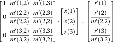
Gaussian elimination is a two‐part procedure that solves for the x‐values of equation set (C3). The result of the first part of the procedure is to convert the system to one in which the elements of the matrix are unity along the main diagonal and zero in the lower triangle.

With this structure the value of x3 is easily obtained from the third equation. ![]() . With x3 evaluated, the second to bottom equation permits a direct calculation for x2. This is the second part of the procedure.
. With x3 evaluated, the second to bottom equation permits a direct calculation for x2. This is the second part of the procedure.
The first part of the procedure is to convert the equation set into the desired form.
C.2.1 Part 1
- Stage 1
- Normalize each of the coefficients in the first column to unity (1.0000…) by dividing all elements in the each equation (coefficients and RHS) by the first coefficient in that equation:(C6)

- Starting with row 2, subtract row 1 from row 2, and then do the same for each subsequent row:(C7)

- For convenience, at the end of this first stage, represent the coefficients and RHS values with a prime:(C8)

- Normalize each of the coefficients in the first column to unity (1.0000…) by dividing all elements in the each equation (coefficients and RHS) by the first coefficient in that equation:
- Stage 2
- Normalize coefficients in the second column (starting with the second row) to unity by dividing each element in the equation by the second coefficient. Do this for all N – 1 rows starting with the second:(C9)
- Subtract the second row from each lower row:(C10)

- And rename the coefficients with a double prime:(C11)

- Normalize coefficients in the second column (starting with the second row) to unity by dividing each element in the equation by the second coefficient. Do this for all N – 1 rows starting with the second:
- Stage 3 (The Last Stage in an N = 3 Equation Set)
- Normalize remaining coefficient in last row:(C12)

- And relabel the coefficient that has been adjusted a third time: (C13)

This is the desired structure that permits a simple step‐by‐step solution.
Note: If there were N equations, this first part would have N stages.
- Normalize remaining coefficient in last row:
C.2.2 Part 2
Solve for each variable in reverse order:
C.3 Pivoting
That was easy! However, there could be a problem if a leading coefficient is zero. Then you have a divide by zero in the normalization (A‐steps) of each stage. Even if the original coefficient value is not zero, this could happen because it becomes zero after the stages. The solution is to resort the columns to make leading coefficient not zero. Better yet, prior to each A‐step, sort the columns so that coefficient with the maximum absolute value is the lead, then this minimizes the effects of truncation error in calculations. This is termed pivoting.
For example, an original equation set might be

The A‐step would direct that all elements in the first equation are to be divided by the x‐coefficient value of “+3.” But the z‐coefficient value of “–10” has a larger absolute value. Accordingly, rearrange the equation set so that z is the first unknown variable in the list. This does not change the solution to the equations:

Note: The elements in the unknown vector have shifted order from (x, y, z) to (z, y, x). In matrix–vector notation,

Switching coefficients to make the leading one the maximum requires switching all column elements in the coefficients matrix and row elements in solution column vector.
For simplicity, there is no need to normalize every successive row, just the one you’re leaving, and then subtract that row times the leading coefficient:


If a divide by zero occurs, it is because the solution is indeterminate (if two or more equations are linearly dependent). So, if a leading coefficient is zero (or equivalently zero numerically, for instance, its absolute value is less than 0.00000001), then send an “indeterminate” message and stop execution.
Since the rows operated on are at the stage number or higher, this procedure can be expressed in pseudocode.
- Stage 1
- Pivot on maximum coefficient in row 1.
- Normalize row 1 with m(1, 1).
- For each subsequent row (index = 2, 3, 4, …), subtract row 1 * m(index, 2) from it.
- Stage 2
- Pivot on max coefficient value in row 2, but only have to search m(2, 2), m(2, 3), …
- Normalize row 2 with m(2, 2).
- For each subsequent row (index = 3, 4,…), subtract row 2 * m(index, 3) from it.
- In general
- Stage k
- Pivot on max coefficient value in row k, but only need to search m(k, k), m(k, k + 1), m(k, k + 2), …, m(k, n).
- Normalize row k with m(k, k).
- For each subsequent
 , subtract
  from it.
Since pivoting scrambles the solution position in the solution vector, the answer needs to be unscrambled. In the example, in Equation (C19) the solution {x, y, z} became reordered as {z, y, x}. To keep track of the order of elements in the solution vector, I use a place vector, in which place holds the original element index.
For example, place is initialized as

After the pivot, x and z are switched so the place vector becomes

There is no need to have an M matrix and an M′ matrix and an M″ matrix. Since each matrix and RHS vector operations update elements, just update the m element.
For example,
The “:=” acknowledges that this is a computer assignment statement, not the algebraic “equals.”
This column switching in the coefficient matrix to make the leading coefficient of the top working row be the coefficient with largest magnitude (absolute value) is called partial pivoting. Full pivoting also switches working rows so that the divide by value in the upper left of the working part of the matrix is the largest magnitude of all remaining in the working matrix.
C.4 Code in VBA
' Gauss Elimination with Pivoting' R. Russell Rhinehart' 29 June 2009, 23 Aug 2012' Gauss Elimination of a system of N (up to 10) linear equations with pivoting on lead coefficientOption ExplicitDim H(10, 10) As Double ' Coefficient Matrix - Hessian in Newton-RaphsonDim V(10) As Double ' RHS vector - Jacobean or Gradient in Newton-RaphsonDim X(10) As Double ' Vector of Unknowns - Change in Decision Variables in OptimizationDim XS(10) As Double ' Scrambled Vector of UnkownsDim Place(10) As Integer ' Position of solution vectorDim TC As Double ' Temporary holder for coefficient value for switchingDim TI As Integer ' Temporary value of column index when switching or unscramblingDim Nvar As Integer ' Number of variables, length of solution vectorDim i As Integer ' index counter for rowDim k As Integer ' index counter for rowDim j As Integer ' index counter for columnDim MaxCoefficient As Double ' value for largest coefficient in the rowDim Index As Integer ' k-value for largest coefficientDim Coefficient As Double ' value of rearragned equation lead coefficientDim sum As Double ' Sum of values in reconstructing the solutionSub Gauss_Elimination_w_Pivot()Nvar = Cells(17, 13)' Initialize sequence of solution vector elementsFor i = 1 To NvarPlace(i) = iNext i' Read DataFor i = 1 To NvarFor j = 1 To NvarH(i, j) = Cells(i + 5, j + 1)Next jNext iFor i = 1 To NvarV(i) = Cells(i + 5, 13)Next i' Perform row operations to get upper-right diagonal matrixFor k = 1 To Nvar - 1' Search for largest coefficient in row kMaxCoefficient = Abs(H(k, k))Index = kFor j = k + 1 To NvarIf Abs(H(k, j)) > MaxCoefficient ThenMaxCoefficient = Abs(H(k, j))Index = jEnd IfNext j' switch Index and k columnsFor i = 1 To NvarTC = H(i, Index)H(i, Index) = H(i, k)H(i, k) = TCNext iTI = Place(Index)Place(Index) = Place(k)Place(k) = TI' normalize lead coefficient of row k to unity - make H(k,k) = 1Coefficient = H(k, k)If Abs(Coefficient) < 0.0000000001 Then 'test for linearly dependent equations.For i = 1 To NvarCells(i + 5, 17) = "Indeterminate"Next iEndEnd IfFor j = 1 To NvarH(k, j) = H(k, j) / CoefficientNext jV(k) = V(k) / Coefficient' subtract row-k-times-lead-coefficient in each remaining row (i>k) - make M(i,k) = 0For i = k + 1 To NvarCoefficient = H(i, k)For j = 1 To NvarH(i, j) = H(i, j) - H(k, j) * CoefficientNext jV(i) = V(i) - V(k) * CoefficientNext iNext k' normalize last row - row i=NvarCoefficient = H(Nvar, Nvar)If Abs(Coefficient) < 0.0000000001 ThenFor i = 1 To NvarCells(i + 5, 17) = "Indeterminate"Next iEndEnd IfFor j = 1 To NvarH(Nvar, j) = H(Nvar, j) / CoefficientNext jV(Nvar) = V(Nvar) / Coefficient' solve for scrambled solution valuesXS(Nvar) = V(Nvar)For j = Nvar - 1 To 1 Step -1sum = 0For k = j + 1 To Nvarsum = sum + XS(k) * H(j, k)Next kXS(j) = V(j) - sumNext j' Unscramble solutionFor i = 1 To NvarTI = Place(i)X(TI) = XS(i)Next i' Display answerFor i = 1 To NvarCells(i + 5, 17) = X(i)Next i' check if solution vector returns RHS vector' Re-read original matrix coefficientsFor i = 1 To NvarFor j = 1 To NvarH(i, j) = Cells(i + 5, j + 1)Next jNext i' Calculate and display RHSFor i = 1 To Nvarsum = 0For j = 1 To Nvarsum = sum + X(j) * H(i, j)Next jCells(i + 5, 14) = sumNext iEnd SubSub GenerateRHS()Nvar = Cells(17, 13)For i = 1 To NvarFor j = 1 To NvarH(i, j) = Cells(i + 5, j + 1)Next jX(i) = Cells(i + 5, 18)Next i' Calculate and display RHSFor i = 1 To Nvarsum = 0For j = 1 To Nvarsum = sum + X(j) * H(i, j)Next jCells(i + 5, 13) = sumNext iEnd Sub