29.1 Introduction

This chapter is a summary of key issues and solutions related to nonlinear regression–fitting nonlinear models to data. The details of diverse issues are revealed in the book Nonlinear Regression Modeling for Engineering Applications: Modeling, Model Validation, and Enabling Design of Experiments by Rhinehart, R. R., John Wiley & Sons, Inc., Hoboken, NJ, 2016b. Here, they are summarized and presented with an optimization application perspective.

Regression is the procedure of fitting a model to data and gives rise to the following optimization questions:

1. Classic nonlinear regression procedures direct the user to transform the model so that linear regression can be applied. Should one?
2. In regression with dynamic models, it is not uncommon to have a delay, an integer multiple of time‐sampling intervals. If delay is a DV, then it is a discretized variable. Compounding the associated difficulties, in regression of nonlinear models, the continuum variables can be constrained, and the models have discontinuities. What optimization method is best?
3. Classically, regression minimizes the squared deviation between model and experimental response, the vertical deviation. This presumes that there is no uncertainty on the input variables and that the y‐variance is uniform over all data. Often these are not reasonable assumptions, and maximum likelihood is a better concept to use. But maximum likelihood is computationally complex. Is there a useful compromise technique?
4. Classic convergence in regression is based on incremental changes in the model coefficients. But how should the thresholds be selected? A better technique is to claim convergence when there is statistically no improvement in the model w.r.t. natural data variability. How should the variability be determined?
5. Often in empirical modeling we progressively add flexibility to a model (perhaps by adding power series terms, or by adding hidden neurons, or by adding logical rules), but improved model flexibility comes at the cost of increasing complexity. We wish goodness of fit to be balanced by model simplicity. What is the OF for determining model order?

29.2 Perspective

Some ask why use sum of squared deviations as opposed to the sum of absolute values of deviations as the objective function in regression. Both objective functions (both measures of undesirability) will work. Both provide reasonable fits of model to data. Minimizing absolute value of the deviations is intuitive, and it seems reasonable. Theoretically, however, as Section 29.5 shows, the sum of squared residuals is grounded in the normal (Gaussian) distribution associated with data variation. If the model is true to the phenomena, and the data are perturbed by many small, equivalent, random, independent influences, then the residuals (data to model deviation) should be Gaussian distributed. Maximizing the likelihood that the model represents the process that could have generated the data, can be functionally transformed, and is equivalent to minimizing the sum of squared residuals.

Additionally, the sum of squares method is continuous with continuous derivatives. The absolute value of the deviation has a slope discontinuity, which can confound classic optimizers (such as Newton types and successive quadratic).

For those two reasons, the classic method, the method used by most modeling software providers, is to minimize sum of squared residuals.

Neither, however, gives the true model. Even if the model were functionally perfect, the perturbations in the experimental data would cause errors. Remove one data and replace it with another data point supposedly at the same conditions. The new one will not be in the same exact place, and the new model will be a bit different.

Further, the truth about nature is elusive. While the model may provide adequate, close enough functionality for engineering utility, and regression may find the best coefficients for the model, the model remains wrong. All we can hope for is a surrogate model that reasonably matches the data. Either minimizing the sum of squared residuals or the sum of absolute values of the deviations provides reasonable models.

29.3 Least Squares Regression: Traditional View on Linear Model Parameters

The objective is to obtain a model that best fits data from an experimental response. First, generate data experimentally. Run an experiment. “Dial in” input conditions, x, measure the response, y. Then find the best model, . The tilde over the f and y explicitly indicates that it is the model, a mathematical approximation, not the true description of Nature. The vector c represents the model coefficients.

Models can have many functional forms. Here are four of an infinite number of common empirical choices for a y‐response to a single x‐variable. The coefficients are a, b, c, d, e. The user must decide on the functional relations appropriate to the application:

(29.1a)

(29.1b)

(29.1c)

(29.1d)

The optimization statement is

(29.2)

where the index i represents data set number. Note that coefficient values, c, and model functionality, , are common to all of the i‐data points.

Classically, we formulate the model to be linear in the coefficients, linear in the DVs for optimization. Then we can use linear regression techniques and have the convenience of knowing that there is one unique solution and that the DV values can be explicitly computed.

A model is linear in coefficients if the modeled response is independently linear to each coefficient—or if the second derivative w.r.t. any combination of coefficients is zero:

(29.3)

The four models are all linear in coefficients a, b, c, d, e. The advantage of this is that the analytical method can be used to determine model coefficient values. Set the derivative of the OF w.r.t. each DV to zero:

(29.4)

This results in N linear equations, each linear in the N DVs. For example, in the quadratic model, , the three derivatives can be rearranged to this set of linear equations in the three coefficients:

(29.5)

(29.5b)

(29.5c)

This set of equations is known as the “normal equations,” and regardless of the number of DVs, it can be represented as , for conventional linear algebra solution.

29.4 Models Nonlinear in DV

However, often, models are nonlinear in the coefficients. Here are three examples:

(29.6a)

(29.6b)

(29.6c)

The optimization statement is still the same:

(29.7)

where the index i represents data set number. Again, the coefficient values, c, and model functionality, , are common to all of the i‐data points.

Classically, we formulate the model to be linear in the coefficients; however, the power law and exponential models are not.

A common linearizing transform for a power law model, , is to log‐transform it:

(29.8)

The relation between and x′ is now linear in coefficients a′ and p. The optimization application becomes

(29.9)

Once linear regression is performed on the transformed data, inverting the transform will return the desired coefficient values. For example, once the value for a′ has been determined, .

There are a wide variety of linearizing transforms for the variety of model functionalities, and conventional practice has offered such as the right way to solve the regression problem. But what is accepted as best in human history has changed from the precomputer era to today. Once, the convenience of linear calculations overrode the desire for model fidelity. Now, I think with the convenience of nonlinear regression model fidelity can be preserved.

Chapter 16 showed that log‐transforming an OF is a strictly positive transformation that does not change the DV values. The log‐transform of the OF would mean

(29.10)

However, log‐transforming the individual data changes the OF:

(29.11)

You can represent this as a weighted least squares OF, where the original OF terms are weighted by a factor, λ_i:

(29.12)

Using the linearized model , then the weighting factor is

(29.13)

The weighting factor depends on both the value of y and the deviation between model and data. It is not a uniform value over all data sets. The DV solutions from the original nonlinear statement of Equation (29.10) and the optimization using the linearizing transforms of Equation (29.11) return different DV values (model coefficient values).

If, however, the model truly represents the data, and the experimental error is small and/or the range is large, then the deviation between the nonlinear and linearized DV values is small. Linearizing transforms have served mankind well, but it should not be considered as best with today’s tools. To prevent the distortion of data importance that results from linearization, do not linearize. Use a numerical optimization method on the nonlinearized data.

29.4.1 Models with a Delay

The model might represent how a process evolves over time. If first order and linear, the ordinary differential equation would be

(29.14)

Alternately, the explicit finite difference representation (Euler’s method) would be

(29.15)

Or the equivalent autoregressive moving average (ARMA) representation is

(29.16)

Here the subscript i indicates the sampling interval, and time is the product of the sample interval number and the time increment, . If the solution to the differential equation is numerical, then Equations (29.15) and (29.16) represent the model. Or if the process data were to be periodically sampled, then values would only exist at discrete time values. In either case, the variable, i, has integer values, and time is discretized.

If not first order or linear, the discretized models are more complicated, but the discretization aspect remains.

There may be a delay between the model input and the impact on its output. For instance, charging on a credit card today has no immediate impact on your bank account, but after the time delay, you have to pay the bill. Then it has impact. Similarly, eating does not nourish the body until after the food is digested and moved to where sugars can be absorbed. There is a delay. Delays can also be due to information or material transfer in a process or communication system.

If first order, linear, and with a delay, the ordinary differential equation would be

(29.17)

Alternately, the explicit finite difference representation (Euler’s method) would be

(29.18)

Or the equivalent autoregressive moving average (ARMA) representation is

(29.19)

Here n represents the number of samplings that equal the delay , but n must be an integer either for either numerical solution or for matching model to sampled data. In the model, θ, or equivalently n, is a coefficient with unknown value to be determined by regression:

(29.20)

Even if the model was classified as linear in ODE terminology (meaning that the principle of superposition can be applied to devise a complete analytical solution as the sum of elements), the regression exercise is nonlinear in how θ, or equivalently n, appears in the model. Not only is the DV discretized to integer values, but it also has a nonlinear impact on the OF. Further complicating things, the data prior to n samplings cannot be used to calculate the OF, because the model does not have u‐data prior to . So, the trial solution for n affects how many elements are in the OF sum.

That was for a dynamic model, but the issues are similar even if the model represents a process for which there is no dynamic evolution, just a delay. This could represent a pipeline transport with plug flow:

(29.21)

Again, even if the model might be linear in the other coefficients, it is nonlinear in the impact of n on the model. Accordingly the optimization is nonlinear, and the DV is discretized.

For such, I recommend a direct search technique with multiple players.

29.5 Maximum Likelihood

We usually pretend (we often say “assume,” “accept,” “given,” or “imply”) that the value of x, wherein the influence on an experiment was perfectly known, was exactly implemented and has no uncertainty. Usually, experimental uncertainty is wholly allocated to the response variable, as the concept is illustrated in Figure 29.1.

Further, we often pretend that the total uncertainty in the location of the data pair is due to random, independent, symmetrically distributed, often Gaussian measurement noise ony.

My use of the term pretend is a bit stronger than most would prefer to use. It does imply a purposeful misrepresentation. But is not the alternate statement “assume the basis for this analysis” also a purposeful misrepresentation? Anyway, don’t use the word pretend when you describe your work. Consider the impact on your audience, and use a term that seems to provide a legitimate underpinning for the assumptions and simplification choices that you made to permit the analysis.

I think that Figures 29.2 and 29.3 provide a truer representation for an experimental process.

Both figures illustrate uncertainty on the measured response, y_meas, as a perturbation being added to the true y‐value. The uncertainty reflects fluctuation, noise, variation, experimental error, etc.; and it may be independent of the y‐value or scaled with the y‐value. It may be symmetric and Gaussian or from an alternate distribution. When independent for each measurement, it is often called random error. If it is a constant value, uniform over many samplings, then it is termed bias or systematic error.

Both figures also reveal uncertainty impacting the input to the experiment. In Figure 29.2 the experimenter sets an input and reads its value from a scale. The reading has uncertainty, so x‐meas is not the same as the x‐true that influences the process. In Figure 29.3 the experimenter chooses the value for x, x‐nominal and attempts to implement it by adjusting the final control element to make the x‐value match the desired value, but experimental uncertainty makes the true influence to the experiment a bit different. The fluctuation could be a bias or systematic error with a fairly constant value over many samplings; alternately it could be independent for each sampling representing random noise effects.

Returning to uncertainty on the y‐measurement, normally, it is considered to represent the uncertainty surrounding the measurement, or lab procedure, or analytical device. But partly, fluctuation on y‐meas is due to uncontrolled experimental aspects that make y‐true vary. Uncontrolled disturbances and environmental effects include raw material variability, relative humidity, electrical charge, experimenter fatigue, air pressure, etc. Certainly, one can model fluctuation to other inputs to the process in a manner of modeling the vagaries on the x‐inputs. But this analysis will pretend that uncertainty on those uncontrolled fluctuations is included in the uncertainty on y‐meas.

With this concept of variation on both the independent and dependent variables, consider the illustration of one data pair in Figure 29.4. The point indicates the experimental values, but the possible true values for either x or y could come from a distribution about the point. Frequently, the variation in either value is the result of many independent, random, and equivalent perturbations, making the distribution normal (Gaussian), as illustrated. The farther away the possible x‐value is from the x‐measurement, the less likely it could have actually generated the x‐measurement. A similar argument goes for the y‐value. Accepting that the x‐variation and y‐variation are independent, the probability that the measured point could have been produced for alternate x‐ and y‐values is the joint probability:

(29.22)

which is illustrated in Figure 29.5.

If Gaussian, the joint probability distribution for the possible location of the point about the measurement (x₀, y₀) is

(29.23)

In maximum likelihood, the objective is to find the model coefficients that maximize the possibility that if the model represented the process, data point (x₀, y₀) could have been the result. The concept is illustrated in Figure 29.6. Note that the points labeled A, B, and C are each on the curve and that point B has the highest likelihood, the highest joint pdf value. There is a possibility that the data point could have been generated from points A and C on the curve, but the point on the curve with the highest likelihood of generating the data point is B. Accordingly, the optimization is a two‐stage procedure. First, choose the model coefficient values, then search along the curve (a univariate search) to find the point of maximum likelihood of generating (x₀, y₀), and label this point on the curve , recognizing that if y is the modeled response to x, the point is .

However, this must be done for each data point. If the variation is independent for all x‐ and y‐values, then

(29.24)

This can be simplified. Since 2πσ_xσ_y is a positive constant, scaling the OF by it does not change the DV* values. Then, since the log‐transformation is a strictly positive transformation, maximizing the product of exponential terms is the same as maximizing the sum of the arguments. Then, since minimizing the negative is the same as maximizing, and since multiplying by 2 does not change the DV* values, the objective becomes

(29.25)

Although simplified, this is still a two‐stage procedure. The outer optimizer assigns values for model coefficients, c. Then for each experimental data set, the inner optimizer performs the univariate search to find the values from which the J_i values can be calculated. The sum of the J_i values is the OF for the outer optimizer.

Note: If the uncertainty on the independent variable is ignored, then , and if σ_y is independent of the y‐values, the OF can be scaled by the positive multiplier, , which reduces the OF to the common vertical least squares minimization.

Note: This can be extended for data and model with multiple x‐values.

Note: Values for σ_y and σ_x need to be known. The values for σ_y and σ_x represent expected variability if all influence values are kept unchanged for replicate measurements. Do not use the standard deviation of the entire list of all the experimental data. Replicate a few conditions at a low medium and high value and evaluate σ_y and σ_x within the replicate sets. Recognize, however, that even with 10 replicated values, there is much uncertainty on the experimentally calculated σ. The 95% confidence limits are roughly between 0.5σ and 2σ.

Note further: It may not be possible to experimentally evaluate the σ_x values, which may have to be estimated using techniques from Chapter 25.

Note: Replicate trials to generate y‐values from which to calculate σ_y, and include the impact of uncertainty on x on the y‐data. However, the concept in Equations (29.23)–(29.25) is that the σ_y value excludes the σ_x effects. Propagation of uncertainty could be used to back out the x‐variability effects on the y‐data.

Fortunately, exact values are not necessary. Classic vertical least squares regression implies that ; and even an approximation of σ_y and σ_x values will allow the maximum likelihood approach to return model coefficient values that are closer to true than does vertical least squares.

However, this two‐stage optimization is somewhat complex, and it is further complicated by removing idealizations used in its development (constant variance, independence of variation, and the Gaussian pdf model). As developed, this has a bunch of pretends and is not perfectly aligned to the maximum likelihood concept. However, it does reveal a method for accommodating independent variable uncertainty; and in my investigations it provides model coefficient values that are closer to true than the simpler vertical least squares. (Such studies must be performed with simulated data, permitting the true coefficient values to be known, so that they can be compared with the regression values.)

Accepting the validity of the simplifications earlier is an optimization exercise. The idealizations simplify the procedure yet retain much of the benefit of the maximum likelihood concept in accommodating the dual uncertainty of both x‐ and y‐values. It is an intuitive conclusion. The traditional least squares OF is opinion based on a diversity of assumptions and only valid if they are true.

29.5.1 Akaho’s Method

Continuing the intuitive evaluation of simplifications that reduce work, yet adequately retain the functionality, I like Akaho’s approximation. It reduces maximum likelihood to a one‐level optimization. Again, the simplification takes the procedure one step further from the ideal concepts; but to me, the benefit (reduction in complexity and computational work) exceeds the loss in veracity of the model coefficient values (as revealed in simulations).

First, scale the x‐ and y‐variables by their estimated standard deviation:

(29.26a)

(29.26b)

(29.26c)

(29.26d)

This makes the likelihood contours become circles with a unit variance, as illustrated in Figure 29.7.

Recall that along a univariate search, the maximum (or minimum) is when the contour is tangent to the line and that steepest descent (or ascent) is ⊥ to the line. For x‐ and y‐variables scaled by σ_x and σ_y, the contours are circular, and the radius is the ⊥ to the circle. That radius is also the shortest distance from the data point to the line.

So, if , then maximum likelihood regression is equivalent to finding the shortest or ⊥ distance to the line. Suppose the x–y relation is a curve. Still, the maximum likelihood for any data point is on a circle that is tangent to the f(x, c ) functions (see Figure 29.8a and b). If it was not tangent, it either crossed the curve or did not touch the curve. Either case means another contour was the one that will be tangent to the function. Then, the best curve, the one maximizing likelihood for the point, is tangent to the likelihood contour, which is a circle. This means that the distance to the point is the radius of the circle, the minimum distance between center and circumference, and that the vector from curve to (x_i y_i) is ⊥ to the curve.

With scaled variables, the maximum likelihood method seeks to find the model coefficient values that minimize the perpendicular distance from the model to the data points, as illustrated in Figure 29.9.

Note: In scaled space the x‐ and y‐variables are dimensionless, and they can be combined into a common dimensionless distance:

(29.27)

The objective is

(29.28)

This is still a two‐stage procedure. The outer optimizer chooses c‐values, then the inner univariate search finds the ‐values that minimize each , and the sum of the values becomes the OF for the search for c‐values.

This approach is variously termed normal least squares, or perpendicular least squares, or total least squares. Be sure to scale the x‐ and y‐variables by their standard deviations so that (i) the likelihood contours are circles and (ii) x and y can be dimensionally combined into a joint distance.

Figure 29.10 illustrates multiple data points and a nonlinear relation graphed on scaled space. Note that the shortest distance between data and model is not the vertical distance. Also note that the direction from the line to data is not the same for each data point and the direction of the normal to the curve changes with position. Finally, note that the curve is not equidistant from the data. Some are on a high contour, and others are on a low contour.

For the special case of a linear relation between y and x, the normal (or ⊥) deviations all have the same slope (the negative reciprocal of the model line). Accordingly, in this special case, the ⊥ deviations are a fixed proportion of the vertical deviations.

Now comes Akaho’s technique that approximates the normal distance and reduces the optimization to a one‐stage procedure. The technique is presented in Figure 29.11.

All are in scaled variables , . This makes the likelihood contours around the appearance of the data point (where measurements or settings make the point appear to be) be concentric circles. Point A is the ith experimental data pair (x_i, y_i), point B is the ith modeled value , and point C is the closest point on the model curve to the experimental data. Because the likelihood contours are circles, line AC is the radius of a circle, and it is perpendicular to every circle perimeter, one of which is the likelihood contour tangent to the curve. So, line AC is also perpendicular to the curve, a normal to the curve. The data pair is a point on the normal or perpendicular line.

The tangent to the model at the modeled , at the ith ׳ value, is illustrated; and point D is the closest point on the tangent line to the data location . Line AD is perpendicular to the tangent line.

Any point on the tangent line can be modeled as a linear deviation from the tangent point along the line of slope S:

(29.29)

is a data pair on the perpendicular to the tangent line from the data apparent location, . It is a radius of the circle centered at the apparent data point location. The slope of a perpendicular line is the negative reciprocal of the tangent line. The relation of any (x,y) pair on the radius line is

(29.30)

At the intersection of the tangent and perpendicular lines, point D, x on the tangent is equal to x on the radius, and y on the tangent is equal to y on the radius. and call them (). Using the two line models, solve for ():

(29.31a)

(29.31b)

The distance from data point to tangent, from point A to D, is

(29.32)

which can be reduced to

(29.33)

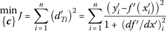
Here the normal distance from data to model is approximated by the vertical distance scaled by the slope of the model. Once the optimizer chooses c‐values, and df ′/dx′ are directly calculated. The inside search for each of the ith points on the model is avoided. Accordingly, Akaho’s approximation to the maximum likelihood optimization is a one‐stage procedure:

(29.34)

For a model with multiple inputs, the method is

(29.35)

The advantage is that Akaho’s method accounts for x‐variability but does not require the nested optimization needed to maximize likelihood or to minimize total least squares. It is a single‐level optimization.

The disadvantage is that this simplification of maximum likelihood assumes constant σ_y and σ_x throughout the range and known values for σ_y and σ_x. Further Akaho’s approximation is not good if curvature makes tangent not represent the distance. See Figure 29.12, where the tangent is a considerable departure from the curve. So, y‐ and x‐uncertainty, σ_y and σ_x, should be small relative to how curvature changes the model.

However, in my opinion, Akaho’s method is fully adequate as a replacement for maximum likelihood, especially when considering the myriad of presumptions related to known sigma values, pdf models, linearity, fidelity of the model to the true natural phenomena, etc.

29.6 Convergence Criterion

Whether using conventional vertical least squares or a maximum likelihood version in nonlinear optimization, traditional convergence criteria for the optimization would be on etc. As ever in optimization, choosing right values for the thresholds on any of those requires understanding of the sensitivity of J to each c and/or to the relative improvement in J or c. These thresholds are scale dependent. They would also be dependent on the sensitivity of the model to the coefficient value. Such aspects confound the user in making a right choice of the threshold.

Further, if the data are very noisy, there should be no pretense about being able to know the truth of the function parameter values, and convergence criteria might as well be “loose.” However, if the noise amplitude is small, then it is reasonable to “see” the model with greater precision, and threshold convergence criteria could be justifiably small. Reasonable convergence criteria should be relative to the noise on the data, which masks the truth. This is illustrated in Figure 29.13, where model (i) is as good as (ii) within the range. The choice of either model is irrelevant considering the data scatter. As a thought exercise, change the location of a data point, reflecting an alternate realization, and consider the impact on the model location.

However, if the variation in the data was much lower, then the data might reveal one model is superior to another. Less variation would also more precisely place the model.

The question is, “How does one set thresholds appropriate to achieving best precision (as justified by variation in the data—noise, uncertainty, fluctuation, or random error) with minimum optimizer work?” An answer is “When model improvement is inconsequential to inherent variability in residuals (data from model), then claim convergence.”

Consider the objective function, for example, the sum of squared deviations (SSD) or its root mean value (rms), as a measure of improvement with iteration:

(29.41)

(29.42)

Figure 29.14 reveals how J might improve with optimization stages. As iterations progress, the SSD or rms progressively drops to its best possible value for the variability in the data and the imperfection in the model.

Since when , alternately when , claim convergence and stop. If a single TS algorithm, use the iteration‐to‐iteration change in the rms. However, if a multiplayer algorithm, use the rms range of players after an iteration. This is a convergence criterion based on the relative change of the OF.

By contrast, as a convergence criterion, at each iteration, measure SSD or rms on a random sampling of about one‐third of the data. (Here, I use random to mean without replacement. Don’t sample a point twice, but I’m not sure that the computational overhead of managing the “no resampling” has any real benefit. In bootstrapping, the data is sampled with replacement.)

(29.43)

Figure 29.15 shows how the rms_random value changes with iteration. In general there is a reduction with iteration as the optimizer improves the model, but the random sampling makes it a noisy trend. At some point, the progressive improvement is inconsequential to the noise on the rms_random signal; at some point the rms_random value comes to steady state w.r.t. iteration. This would indicate that there is no meaningful improvement in the model relative to data variability, and convergence should be claimed.

Use any technique you prefer to identify steady state to the rms_random w.r.t. iteration trend. My choice is the ratio of filtered variances of Cao and Rhinehart (1995). Since the sampling is random, at steady state the “noise” on the rms subset is independent from iteration to iteration, which satisfies the basis of their technique. This is a scale‐free approach. If you change the units, the ratio remains dimensionless with the same threshold value. The threshold value required to detect SS is independent of the number of DVs or whether the stochastic nature is due to Monte Carlo simulation, experimental outcomes, or random data subset sampling. It is relatively independent of the distribution of the deviations. It is a computationally simple approach. Details are described in Appendix D. Here is a summary. Measure the variation from the average in about the past 10 data iterations, and measure the variation along the trend, as shown in Figures 29.16 (Not at SS) and 29.17 (At SS).

When not at SS, the deviation from average is much greater than deviation from a trend line:

(29.44)

By contrast, when at SS, the deviation from average is indistinguishable from deviation from the trend:

(29.45)

Traditional methods use the sum of all data to calculate the signal values, which is a computational burden. It requires storage of N past data and updating sum of squared deviations at each iteration. So revisit the concept of calculating the variance, and use a first‐order filter approach:

(29.46)

There is a relation between λ, the number of data, and a time constant for the filter:

(29.47)

Equation (29.46) is also called an exponentially weighted moving average (EWMA).

The expectation (the mean or many data average value) on x_f is the expectation on average value, which is the average:

(29.48)

It doesn’t matter what quantity x represents. Normally, it represents an individual measurement. But it could represent a scaled variable, or a deviation, or a deviation squared. If defined as the first‐order filter of the squared deviation from the average, it is termed an exponentially weighted moving variance (EWMV):

(29.49)

Instead of using use the computationally simpler x_f. In the following equations, is the measure of variance between data and average used in the numerator, and is the measure of the variance inherent in the data (between successive data) and used in the denominator:

(29.50)

(29.50b)

(29.50c)

(29.50d)

The filter on x is performed after calculating the numerator measure of variance to eliminate correlation of to x_i. Otherwise, the r‐statistic is more complicated. To return the ratio to represent the variance ratio, it needs to be scaled by (2 − λ₁). If , then the trend is in a transient. If , then the trend is in a steady state. Since data vagaries cause the statistic to vary when the signal is at SS, the values for r_i range between about 0.8 and 1.5. Accordingly, if , then accept that the trend is at SS. I initialize all values with zero.

Figure 29.18 illustrates the distribution of the r‐statistic when a signal is not at SS (right‐hand curve) and all r‐statistic values are greater than 3. The left‐hand curve shows the distribution of the r‐statistic when the process is at SS. Note that half of the values are above the ideal value of 1 and half below. The middle curve shows the distribution for a signal that is nearly, but not quite at SS. Note that the almost at SS signal has occasional r‐statistic values of less than 1, but it does not place values in the 0.85 region. Accordingly, 0.85 is a useful trigger to determine SS. I use 0.80 when I want to be very sure and 0.9 if less strict.

Since , effectively in filtering number of data the window that is observed. Ten to 20 data points is a reasonable quantity.

I have been fairly satisfied with and . When the process is at SS, these values will claim steady state faster (fewer iterations). However, they may accept a near to steady state, but not quite there process as at steady state. You might want to use those values when exploring or screening to make a sequence of trials end in less time. However, and values will provide greater assurance that the procedure has really achieved steady state. Although they will require more iterations, they provide greater confidence that a type II error is not being made.

If optimization starts either far from optimum on a very flat surface, or if the optimizer is just getting adjusted to the right step sizes to make progress, then the initial progress in OF w.r.t. iteration could be slow. As Figure 29.19 illustrates, the initial iterations may not reveal a substantial improvement.

Exploring options for using SS to claim convergence, one approach is to not start testing for SS until after there is confidence that a transient has happened. However, if by chance the initial trial solution is very near the optimum, it will not detect a transient; then never begin testing for SS, and run the maximum iterations. I find that initializing all variables with zero is a great solution. First, it is simple. There is no need to collect N data to initialize values for , , or x_fi. Second, even if the optimizer initial trial solution fortuitously defined the correct model, the SSID initialization makes it appear that there is an initial transient as , , and x_fi approach their steady values.

29.7 Model Order or Complexity

Regardless of the optimizer choice, objective function choice, or method of convergence, the user makes choices with regard to the model. If the model is phenomenological (indicating that the user chose a mechanistic, or first principles approach), then the model structure is fixed. However, if the user chooses empirical modeling, the question is, “What order to use?” Nominally this would mean “What powers of x are to be used.” But also this could mean how many wavelets, or how many neurons in the hidden layer, or how many categories in a fuzzy logic linguistic partition, or how many sampling intervals in an ARMA model, or how many orthogonal polynomials.

A Taylor series analysis indicates a power series is “right” for any relation. For a y‐response to a single x‐independent variable, the series is

(29.51)

Although the derivatives seem like a function, they are evaluated at the single base point, x₀. Accordingly, they are coefficients in the model with constant values. By grouping coefficients of like powers of x, one obtains the classic power series model:

(29.52)

Again, in empirical modeling, the question is, “What model order is right?” In empirical regression, if there are too many model coefficients, the model can fit the noise and provide a ridiculous representation of the process. In Figure 29.20, the true y(x) relation is represented by the dashed line. It is the unknowable truth about nature. The dots represent the results of five trials to generate y‐values from x‐values. The solid line is a five‐coefficient (fourth‐order) polynomial model fit to the data. It exactly goes through each data point, but it is a ridiculous model. It fits the noise and does not reveal the underlying trend. Depending on the discipline, this is termed “memorization” or “overfitting.”

A classic regression modeling heuristic to prevent overfitting is to have three (or more) data pairs per model coefficient. Then, to balance the work and cost associated with generating data, if three experimental sets per model coefficient are adequate, then do not generate more than three per coefficient. So, for six data points you should only consider a two‐parameter (linear) model. If there are 15 data points, you could use a 5‐parameter (quartic) model. This heuristic does not say that a quartic model is right. Perhaps a linear model would be better.

What does better mean?

• More representative of an intuitive understanding of behavior (trends and extrapolation)?
• More functional in use (invertible with a unique solution)?
• More sufficient (meets customer specifications for variance)?
• Lower cost?

You should consider what issues constitute complexity/simplicity and desirability/undesirability in your application and add your perspectives to this list.

Many people have investigated this issue and devised a variety of metrics to assess complexity of a regression model. What follows is one approach that looks at one metric for model goodness of fit and relative complexity.

Let’s look at variance reduction as a measure of goodness of fit. The commonly used r² is a measure of SSD reduction, but does not account for the degrees of freedom in the variance:

(29.53)

(29.54)

A total reduction of residual variability, a perfect fit to the data, would result in . However, a perfect value of unity does not mean that the model is right. The basic model architecture could be wrong. For example, if the unknowable truth is , and noisy data is generated within the to region, the graph may appear to be the left half of a parabola (see Figure 29.21), and a quadratic model may seem to provide a reasonable fit.

Model goodness of fit will be evaluated by SSD_residuals. How will complexity be assessed? Using N as the number of data sets and m as the number of model coefficients, the quantity represents the total work related to number of experiments and modeling effort. The quantity N − m represents the degrees of freedom. The ratio represents the effort‐to‐freedom aspect. Consider that the model has m coefficients. For a quadratic model (order 2 in the independent variable), there are coefficients. In a sixth‐order polynomial, there are coefficients.

There are several methods to balance improvement of fit relative to model complexity, as measured by number of coefficients, m. A simple one is the final prediction error (FPE) criterion, originally introduced by Akiake, but promoted and brought to wider acceptance by Ljung (in the 1980–2000 period, about 15 years later):

(29.55)

(29.56)

The procedure is to start with a low order model, small m, and progressively add coefficients (terms or functionalities) until FPE rises. As m increases from an initial small value, the model will get better, and SSD will drop. Initially, usually, the reduction in SSD will be greater than the increase in the complexity factor, and FPE will drop with increasing m. Incrementally increase m until FPE rises, which indicates that the previous m was best. This is a univariate optimization with an integer DV:

(29.57)

Note: It does not have to be a power series model as I’ve been illustrating. It could be a neural network model (adding hidden neurons) or a first principles model (adding nuances).

This FPE optimization does not provide the values for the model coefficients, just the model order. Choose an m, model order. Use regression to determine coefficient values, and calculate FPE. Choose another m, and repeat. This is a nested optimization.

Given a model architecture and number of coefficients, m, any optimization technique could be used to find the model coefficient values:

(29.58)

Regardless of the choice of optimization technique (successive quadratic, Cauchy, LM, NM Simplex, Hooke–Jeeves, leapfrogging, … or classic analytical), they should find the same best coefficient set values. Which optimization technique is used to determine the {a, b, c, d, …} values is irrelevant to the decisions about model architecture or the use of FPE to determine the correct model order.

If you have a mechanistic model (first principles, phenomenological, physical), use it. The Taylor series expansion is mathematically defensible and indicates that your phenomenological model can be converted to a power series. If you have no concept of the mechanistic model, then an empirical model is permissible. But if you have a phenomenological understanding, use it. A phenomenological model has fewer coefficients. A phenomenological model extrapolates. A phenomenological model represents the best of human understanding. Don’t use … to override phenomenological models.

If your modeling software does not provide SSD, but provides the r‐square value, you can use the r² value instead of SSD in FPE. From the definition of r²,

(29.59)

This can be solved for SSD:

(29.60)

Substituting in the FPE equation,

(29.61)

The objective is to find the number of model coefficients to minimize FPE:

(29.62)

Since SSD_{original data} is a positive‐valued constant, scaling the OF by it does not change the m* value. So,

(29.63)

The SSD_{original data} value is not needed.

FPE is one approach to determining a balance between model complexity and goodness of fit. Many others have been developed and promoted. There are alternate measures of the desirables and undesirables and alternate ways to combine the balance. My personal experience is that FPE (and similar methods that only look at the SSD and number of model coefficients relative to number of data) permit greater empirical model complexity than I often prefer. Accordingly, I like an equal concern approach, because I can adjust the weighting based on my feel about the application:

(29.64)

Regardless, I like FPE for its simplicity and general relevance if the user does not have specific and alternate views about the balance of desirables.

Also, I like FPE because it reveals a nonadditive approach to combining the several OF considerations.

29.8 Bootstrapping to Reveal Model Uncertainty

Uncertainty in experimental data leads to uncertainty on the regression model coefficient values, which leads to uncertainty in the model‐calculated outcomes. We need a procedure to propagate the uncertainty in experimental data to that on the modeled values, so these aspects of model uncertainty can be appropriately reported.

In linear regression, this is relatively straightforward, and mathematical analysis leads to methods for calculating the standard error of the estimate and the 95% confidence limits on the model. However, the techniques are valid only if the following conditions are true: (i) the model functional form matches the experimental phenomena; (ii) the residuals are normally distributed because the experimental vagaries are the confluence of many, small, independent, equivalent sources of variation; (iii) model coefficients are linearly expressed in the model; and (iv) experimental variance is uniform over all of the range (homoscedastic), and then analytical statistical techniques have been developed to propagate experimental uncertainty to provide estimates of uncertainty on model coefficient values and on the model.

However, if the variation is not normally distributed, if the model is nonlinear in coefficients, if variance is not homoscedastic, or if the model does not exactly match the underlying phenomena, then the analytical techniques are not applicable. In this case numerical techniques are needed to estimate model uncertainty. Bootstrapping is the one I prefer. It seems to be understandable, legitimate, and simple and is widely accepted.

Bootstrapping is a numerical Monte Carlo approach that can be used to estimate the confidence limits on a model prediction.

One assumption in bootstrapping is that the experimental data that you have represents the entire population of all data realizations, including all nuances in relative proportion. It is not the entire possible population of infinite experimental runs, but it is a surrogate of the population. A sampling of that data then represents what might be found in an experiment. Another assumption is that the model cannot be rejected by the data, but the model sufficiently expresses the underlying phenomena. In bootstrapping,

1. Sample the experimental data with replacement (retaining all data in the draw‐from original set) to create a new set of data. The new set should have the same number of items in the original, but some items in the new set will likely be duplicates, and some of the original data will be missing. This represents an experimental realization from the surrogate population.
2. Using your preferred nonlinear optimization technique, determine the model coefficient values that best fit the data set realization from step 1. This represents the model that could have been realized.
3. Record the model coefficient values.
4. For independent variable values of interest, determine the modeled response. You might determine the y‐value for each experimental input x‐set. If the model is needed for a range of independent variable values, you might choose 10 x‐values within the range and calculate the model y for each.
5. Record the modeled y‐values for each of the desired x‐values.
6. Repeat steps 1–5 many times (perhaps over 1000).
7. For each x‐value, create a CDF of the 1000 (or so) model predictions recorded in step 5. This will reflect the distribution of model prediction values due to the vagaries in the data sample realizations. The variability of the prediction will indicate the model uncertainty due to the vagaries within the data. For some applications 100 samples may be adequate, and others may require 100,000 samples. When the CDF shape is relatively unchanging with progressively added data (steps 1–5), you’ve done enough.
8. Choose a desired confidence interval value. The 95% range is commonly used.
9. Use the cumulative distribution of model predictions to estimate the confidence interval on the model prediction. If the 95% interval is desired, then the confidence interval will include 95% of the models; or 5% of the modeled y‐values will be outside of the confidence interval. As with common practice, split the too high and too low values into equal probabilities of 2.5% each, and use the 0.025 and 0.975 cdf values to determine the y‐values for the confidence interval.
10. Repeat steps 7–9 for each model coefficient value recorded in step 3 to reveal the uncertainty range on each.

This bootstrapping approach presumes that the original data has enough samples covering all situations so that it represents the entire possible population of data. Then the new sets (sampled with replacement) represent legitimate realizations of sample populations. Accordingly, the distribution of model prediction values from each resampled set represents the distribution that would arise if the true population were independently sampled.

Bootstrapping assumes that the limited data represents the entire population of possible data, that the experimental errors are naturally distributed (there are no outliers or mistakes, not necessarily Gaussian distributed, but the distribution represents random natural influences), and that the functional form of the model matches the process mechanism. Then a random sample from your data would represent a sampling from the population; and for each realization, the model would be right.

If there are N number of original data, then sample N times with replacement. Since the central limit theorem indicates that variability reduces with the square root of N, using the same number keeps the variability between the bootstrapping samples consistent with the original data. In step 1, the assumption is that the sample still represents a possible realization of a legitimate experimental test of the same N. If you use a lower number of data in the sample, M, for instance, then you increase the variability on the model coefficient values. You could accept the central limit theorem and rescale the resulting variability by square root of M/N. But the practice is to use the same sample size as the “population” to reflect the population uncertainty on the model.

In step 6, if only a few resamplings, then there are too few results to be able to claim what the variability is with certainty. As the number of step 6 resamplings increases, the step 9 results will asymptotically approach the representative 95% values. But the exact value after infinite resamplings is not the truth, because it simply reflects the features captured in the surrogate population of the original N data, which is not actually the entire population. So, balance effort with precision. Perhaps 100 resamplings will provide consistency in the results. On the other hand, it is not unusual to have to run 100,000 trials to have Monte Carlo results converge.

One can estimate the number of resamplings, n, needed in step 6 for the results in step 9 to converge from the statistics of proportions. From a binomial distribution, the standard deviation on the proportion, p, is based on the proportion value and the number of data:

(29.65)

Desirably, the uncertainty on the proportion will be a fraction of the proportion:

(29.66)

where the desired value of f might be 0.1.

Solving Equation (29.65) for the number of data required to satisfy Equation (29.66),

(29.67)

If p = 0.025 and f = 0.1, then n ≈ 4000.

Although n = 10,000 trials is not uncommon, and n = 4000 was just determined, I think for most engineering applications 100 resamplings will provide an appropriate balance between computational time and precision. Alternately, you might calculate the 95% confidence limits on the y‐values after each resampling, and stop computing new realizations when there is no meaningful progression in its value, when the confidence limits seem to be approaching a noisy steady‐state value.

In step 9, if you assume that the distribution of the ‐predictions are normally distributed, then you could calculate the standard deviation of the ‐values and use 1.96 times the standard deviation on each model prediction to estimate the 95% probable error on the model at that point due to errors in the data. Here, the term error does not mean mistake; it means random experimental normal fluctuation. The upper and lower 95% limits for the model would be the model value plus/minus the probable error. This is a parametric approach.

By contrast, searching through the n = 4000, or n = 10,000 results to determine the upper and lower 97.5 and 2.5% values is a nonparametric approach. The parametric approach has the advantage that it uses values of all results to compute the standard deviation of the ‐prediction realizations and can get relatively accurate numbers with much fewer number of samples. Perhaps, n = 20. However, the parametric approach presumes that the variability in ‐predictions is Gaussian. It might not be. The nonparametric approach does not make assumptions about the underlying distribution, but only uses two samples to interpolate each of the and values. So, it requires many trials to generate truly representative confidence interval values.

Unfortunately, the model coefficient values are likely to be correlated. This means that if one value needs to be higher to best fit a data sample, then the other will have to be lower. If you plot one coefficient w.r.t. another for the 100 resamplings recorded in step 3 and see a trend, then they are correlated. When the variability on input data values is correlated, the classical methods for propagation of uncertainty are not valid. They assume no correlation in the independent variables in the propagation of uncertainty. Step 10 would have questionable propriety.

Also, step 9 has the implicit assumption that the model matches the data, that the model cannot be rejected by the data, and that the model expresses the underlying phenomena. If the model does not match the data, then bootstrapping still will provide a 95% confidence interval on the model; but you cannot expect that interval to include the 95% of the data. As a caution, if the model does not match the data (if the data rejects the model), then bootstrapping does not indicate the range about your bad model that encompasses the data, the uncertainty of your model predicting the true values.

Figure 29.22 reveals the results of a bootstrapping analysis on a model representing pilot‐scale fluid flow data. The circles represent data, and the inside thin line is the normal least squares modeled value. The darker lines indicate the 95% limits of the model based on 100 bootstrapping realizations evaluated at the x‐values of the data set of 15 elements. (The y‐axis is the valve position and the x‐axis is the desired flow rate. Regression was seeking the model inverse.)

29.8.1 Interpretation of Bootstrapping Analysis

Here is a bootstrapping analysis of the response of electrical conductivity to salt concentration in water. The data in Figure 29.23 are generated with concentration of salt as the independent variable and conductivity as the response; but as an instrument to use conductivity to report salt concentration, the x‐ and y‐axes are switched. The figure represents a calibration graph. The model is a polynomial of order 3 (a cubic power series with four coefficients).

The conductivity measurement results in a composition error of about ±2 mg/dL in the intermediate values and higher at the extremes. The insight is that if ±2 mg/dL is an acceptable uncertainty, then the calibration is good in the intermediate ranges. If not, the experimenters need to take more data to use more points to average out variation. Notice that the uncertainty in concentration has about a ±5 mg/dL value in the extreme low or high values. So, perhaps the experiments need to be controlled so that concentrations are not in the extreme low or high values where there is high uncertainty.

There are five curves in the figure. The middle curve is the best least squares model. It is a continuous function. The extreme curves represent the extreme values of the models, at selected x‐points, from the 100 bootstrapping trials. The extreme curves are a connect‐the‐dots pattern, not a continuous model representation. The close‐to‐extreme curves are connect the dots of the 95% upper and lower model results.

Figure 29.24 is another example of data from calibrating index of refraction with respect to mole fraction of methanol in water. Because the response gives two mole fraction values for one I.R. value, the data represents the original x–y order, not the inverse that is normally used to solve for x given the measurement. This model has a sine functionality, because it gives a better fit than a cubic polynomial.

How to interpret? If the distillation technician takes a sample, measures index of refraction, and gets a value of 1.336, the model (middle of the five curves) indicates that the high methanol composition is about 0.72 mol fraction. But the 95% limits indicate that it might range from about 0.65 to 0.80 mol fraction. This large range indicates that the device calibration produces ±0.07 mole fraction uncertainty or ±10% uncertainty in the data. However, if the index of refraction measurement is 1.339, the model indicates about 0.4 mol fraction, but the uncertainty is from 0.3 to 0.6. Probably, such uncertainty in the mole fraction would be considered too large to be of use in fitting a distillation model to experimental composition data.

Bootstrapping analysis reveals such uncertainty, when it might not be recognized from the data or the nominal model. The model can be substantially improved with a greater number of data in the calibration.

The data in Figures 29.23 and 29.24 was generated by ChE students in the undergraduate unit operations lab at OSU. I greatly appreciate Reed Bastie, Andrea Fenton, and Thomas Lick for sharing their index of refraction data for my algorithm testing and to Carol Abraham, John Hiett, and Emma Orth for sharing their conductivity calibration data. The fact that this analysis suggests that they need more data is not a criticism of what they did. One cannot see how much data is needed until after performing an uncertainty analysis.

Hopefully, these examples help you understand how to use and interpret model uncertainty.

29.9 Perspective

In nonlinear regression you could use any optimizer and any convergence criterion. You could use Levenberg–Marquardt with convergence based on the cumulative sensitivity of the DV changes on the OF. You could use Hooke–Jeeves with convergence based on the pattern exploration size. I use leapfrogging and, for convergence, the steady‐state condition on the random subset rms value. Any combination can be valid.

However, regardless of the optimizer or the convergence criterion, nonlinear regression beats regression on the linear transformed model, because the linear transformations change the weighting on some data points. I strongly encourage you to use nonlinear regression. However, if there is a copious amount of data so that deviations are balanced, or if the variation is small, then linearizing transforms could represent best balance of convenience and sufficiency over perfection.

Regardless of the optimizer there could be local optima traps in nonlinear optimization, so you should use a best‐of‐N‐independent initializations approach. Some people use N = 10. I suggest N = ln(1 − c)/ln(1 − f).

I like nonlinear regression over linear regression on linear transformed models because it is as easy for me and gives results that are truer to reality. I like N = ln(1 − c)/ln(1 − f) because it provides a basis for the value of N. I like leapfrogging because it provides a balance of simplicity and performance (robustness, PNOFE) that wins in most test cases I’ve explored. For regression, I like the convergence criterion based on random subset rms steady‐state condition because it is scale independent, is data based, and does not require a user to have to input any thresholds. I like the r‐statistic filter method for steady‐state identification because it is robust and computationally simple.

Although I think my preferences for nonlinear regression are defensible, they will not be shared by everyone.

The program “Generic LF Static Model Regression” combines what I think are best practices: best of N for repeat runs, steady‐state stopping, and leapfrogging.

29.10 Takeaway

Your model is wrong. First, nature is not bound by your human cause‐and‐effect modeling concept. Second, even if your model could be functionally true, because experimental data are noisy, not exactly reproducible, then a best model through the data will be corrupted by the data variability. For nonlinear models, use a bootstrapping technique to reveal the uncertainty of the model resulting from the data variability.

Vertical least squares minimization is grounded in normal (Gaussian) variability but pretends that all input values are perfectly known. Akaho’s method is a nice simplification of maximum likelihood to account for input uncertainty; but it presumes uniform variance. The classic maximum likelihood technique uses the Gaussian distribution, but alternate models could be used. However, it is a two‐stage optimization procedure, and the conceptual perfection might not be justified by the data‐induced uncertainty in the model, or the necessarily specified estimates for the σ‐values of the input and response variables. For me, Akaho’s method provides the best balance of accounting for input variability with minimum complexity.

Many nonlinear regression applications have a single optimum with a smooth, quadratic‐like response to the model coefficient values. Gradient or second‐order optimization techniques are often excellent. However, as often in my applications, nonlinearities or striations in the response confound gradient and second‐order procedures. In any case the user must choose a convergence criterion and appropriate threshold, which requires a priori knowledge.

For generality (robustness, simplicity, effectiveness), I like LF with best‐of‐N randomized initializations and convergence on the rms of a randomly sampled subset of the data. I like bootstrapping as a method to assess uncertainty of the model due to data variability.

29.11 Exercises

1. Show that you know what the “normal equations” are. You can explain, derive, describe, or whatever; but keep your answer direct to the point and simple.
2. State which is better, and explain why: the use of Σ|d| or Σd² in regression.
3. Figure 29.25 shows a curve fit to three data points. Variables x and y have the same units and scale. Since values for σ_x and σ_y change with x–y position, the likelihood contours are shown with varying aspect ratio. Values 0.7, 0.8, and 0.9 represent the contours of constant likelihood. In a maximum likelihood optimization to best fit the curve to the data, determine the value of the objective function.

   

4. Linearization of a model by log‐transforming the data distorts the data and causes the optimizer to find a set of optimal parameter values that is less true to the underlying trend than when the optimizer uses the untransformed data. What conditions would make such linearization acceptable? Defend your answer.
5. Linearization of a model by log‐transforming the data distorts the data and causes the optimizer to find a set of optimal parameter values that is less true to the underlying trend than when the optimizer uses the untransformed data. But log‐transforming the objective function (a feature taken advantage of in the transformation of maximizing likelihood to minimizing squared deviations) does not change the optimal solution. Explain why one log‐transformation changes the optimal solution but the other does not. You may use equations and sketches to help reveal your explanation.
6. If you did not know the phenomenological functional form of a relation, you could use a power series expression, to generate a ρ(T) relation. How would you determine the number of terms in the power series expansion? Explain.
7. Wikipedia reports that the phenomenological model for temperature dependence of resistivity in noncrystalline semiconductors is where n = 2, 3, or 4 depending on the dimensionality of the system. If you knew that functional relation, you would have one coefficient, A, to fit the model to data. Is that linear or nonlinear regression? Explain.
8. Figure 29.26a is a plot of three data pairs of y versus x. Sketch the linear relation, , that is the best line in a traditional least squares approach (vertical deviations). I suggest you use your pencil as the trial line, move it around to “eyeball” the best line, and then sketch the line. Figure 29.26b indicates likelihood contours about the same three data points. Sketch the linear relation, , that is the best line in a maximum likelihood approach. Again, I suggest you use your pencil as the trial line and move it around to “eyeball” the best line. Discuss the similarity and contrast of the two solutions.

   

9. What limiting conditions would make vertical least squares return just as good a model as maximum likelihood? Defend your answer.
10. FPE is a method to determine when to stop adding functionalities to a model. Can FPE be used if a functionality is a reciprocal or exponential? Consider this question: “The current m = 3 model is , can I use FPE to determine if I should use an m = 4 model of the form ?” Choose, and explain your answer: Yes, No, Possibly.
11. If the logarithm is a strictly positive transformation that converts the maximum likelihood concept to the least squares concept for regression, why should data not be log‐transformed to linearize the model in regression?
12. Use objective function transformations to show how maximizing likelihood becomes minimizing vertical least squares. Start with this optimization statement (a Gaussian likelihood model that assumes no x‐uncertainty and constant y‐variability). The model is a power law model. N is the number of data, and i is the data index:
    
    
13. If the model is , and σ_y and σ_x have different values, but are constant, Akaho’s technique to approximate maximum likelihood scales the variables by the standard deviations, then seeks a solution by the scaled notation below. Unscale the variables to convert this to the user‐familiar variables of .:
    
14. In regression modeling, we often log‐transform a power law model to obtain an equation that is linear in the model coefficients. Then we can apply the analytical least squares of vertical differences approach to generate the “normal equations,” from which linear algebra gives the exact solution for model coefficient values. Quantify the weighting distortion on the squared deviation values due to the log‐transformation.
15. Derive equations that show, for regression to a linear model, minimizing the sum of squared vertical differences between data point and line provides different results from minimizing the sum of squared normal (perpendicular or orthogonal to the regression line) differences.
16. You do not need to understand chemical reactions to do this exercise. A chemical reaction model of a packed‐bed reactor is a follows:
    
    where
    • C_i is the inlet concentration of reactant, gmol/L
    • C_o is the outlet concentration of reactant, gmol/L
    • V is the reactor volume, mL, V = 1000 mL
    • F is the reactant inlet flow rate, mL/s
    • T is the reaction absolute temperature, K
    • R is the gas law constant 8.314, kJ/kmol‐K
    • k₁ is the mass transport resistance coefficient, (gmol/L)⁻¹—nominal range 5–100
    • k₀ is the “pre‐exponential” reaction rate coefficient, s⁻¹—nominal range 0.0001–1
    • E is the reaction activation energy, kJ/kmol—nominal range 5000–40,000

    The unknowns are the values of reaction properties k₁, k₀, and E. Use optimization of the least squares C_o deviations from data to model (vertical deviations) to determine values for the reaction properties k₁, k₀, and E. The known values belong in several categories. The gas law constant, R, is a universal constant of nature. The reactor volume, V, is a physical property of the experimental equipment. Design of the experimental conditions leads to user choices of the three variables: C_i, F, and T. Finally, the response of the reaction system is the measured value for C_o.

    This will be root finding nested with the optimization. Either Newton’s method or successive substitution works well for the root finding. The optimizer will “guess” at values for the three DVs (k₁, k₀, and E). Then root finding is needed to solve for the modeled C_o value. Then the sum of squared deviations in outlet concentration (model minus measured) can be evaluated.

    Use steady state based on random sum squares sampling as the convergence criterion. Use N independent trials to be 99% confident that you’ll have found at least one of the best 1% possible solutions (Table 29.1).

    Run	Nominal			Measurement
    	Ci (gmol/L)	F (ml/s)	T (K)	Co (gmol/L)
    1	0.5	1	300	0.387994
    2	0.5	1	325	0.266296
    3	0.5	1	370	0.194875
    4	0.5	2	300	0.585542
    5	0.5	2	325	0.486686
    6	0.5	2	370	0.283753
    7	0.5	3	300	0.395264
    8	0.5	3	325	0.345275
    9	0.5	3	370	0.394145
    10	1	1	300	0.885848
    11	1	1	325	1.0322
    12	1	1	370	0.595486
    13	1	2	300	0.920307
    14	1	2	325	0.696697
    15	1	2	370	0.948037
    16	1	3	300	0.788529
    17	1	3	325	1.129603
    18	1	3	370	0.881381
    19	2	1	300	1.988986
    20	2	1	325	2.039343
    21	2	1	370	1.48991
    22	2	2	300	2.250937
    23	2	2	325	1.778625
    24	2	2	370	1.646426
    25	2	3	300	2.110882
    26	2	3	325	1.777817
    27	2	3	370	1.99707

17. In regression modeling, we often log‐transform a power law model to obtain an equation that is linear in the model coefficients. Then we can apply the analytical least‐squares‐of‐vertical‐differences approach to generate the “normal equations,” from which linear algebra gives an exact solution for model coefficient values. Alternately, we can use nonlinear numerical optimization techniques to approximate the coefficient values. Nonlinear optimization is more work, but does not cause the distortion of the log‐transformation. Choose coefficient values for your power law. That model represents the unknowable truth about nature. Simulate experimental data. Perform both nonlinear regression and linear regression on the log‐transformed model, with the data, to get model coefficients. Compare results. On a y versus x plot, there is a steep portion of the power law model and a not‐so‐steep portion. Your data points should include both slope regions; otherwise linear regression will be right. If your data has zero noise, then both regression approaches should give identical coefficient values, equaling the true (but unknowable) values; however, the convergence criteria on the numerical algorithm will limit precision. If the noise is too high, neither method will give good values. If there are many data points, then in any one region, “+” and “−” deviations will balance the “pull,” and the linearized approach should not be biased by the weighting distortion. However, if too few (just 2) data points, the two approaches should return identical, but bad wrong, coefficient values. You choose the number, location, and noise aspects of the data so that your comparison of the two regression techniques reflects the method, not the number, placement, and noise on the data. In generating data, be true to reality. Choose a nominal x‐value, but perturb it a bit before calculating the y‐value. Then add noise to the modeled y‐value to represent the measurement. Your data representing your experimental knowledge of the process should be the nominal x‐ and y‐measurement pairs. You cannot know either the actual (perturbed) x‐value or the true y‐value.
18. I claim that FPE is a good method for selecting model order. The method finds the number of model coefficients that minimizes FPE = [(N + m)/(N − m)] * SSD_m. What do you think? Provide evidence to support your conclusion. Here is one approach: use a linear y versus x relation to generate data, and add noise to the y‐data. Then let Excel (or any software) find the best linear model (m = 2), then the best quadratic model (m = 3), then cubic (m = 4), etc. At each m, use the r‐square as a measure of SSD. You can show that SSD_m = SSD₁ * (1 − r‐square_m). Since FPE′, FPE scaled by a positive multiplier, does not change the DV optimum, you can use FPE′ = [(N + m)/(N − m)] * (1 − r‐square_m) versus m to determine the best value of m. Because you know that the generating model was linear, if the method is good, then the results should show that the minimum FPE׳ occurs at m = 2. If the FPE method is good, then the value of m should be consistent with the generating model (e.g. m = 4, if the generating model was cubic). And the approach should be independent of either the number of data, or the amplitude of the noise, or the slope of the generating line, or values of the other model coefficients. I suspect that the results will not be deterministic. You will not get a clear “Yes, it works perfectly, there was no error in the optimum m” result. The statistical vagaries of noise perturbations on the true y‐values in one particular test may make it appear that a cubic model is best when the truth is quadratic. So, your assessment and conclusion as to whether FPE works or not cannot be based on an expectation that the method is universally perfect.
19. I have claimed that the steady‐state identification method is a good approach to detecting convergence in optimization of model coefficient values in nonlinear regression. “Good” means that it works reasonably well, is scale independent, is user convenient, and is grounded in fundamentals. What do you think? Provide evidence to support your conclusion. What makes one method better than another? If the SSID approach is universal (if it is scale independent, and does not require a person to choose threshold values, and does not require adding apples and oranges), then that makes it better than the other approach. If the NOFE is lower for one method than another, while giving the same optimum DV value, then the one method is better. How will you define better? What will you measure to quantify better and to defend your conclusion?
20. Develop an experiment to compare Akaho’s method to approximate total least squares to classic vertical least squares. Here is a guide: generate N (x, y) pairs from the truth about nature (a reference model). Add independent variation to the x‐ and y‐values to obtain the simulated experimental data pairs. Assume that the simulated x‐values are the truth, and use nonlinear regression on the conventional vertical y‐deviations to determine model coefficient values. Also, scale the data with the respective variances. Use nonlinear regression on the Akaho distance to determine scaled model coefficient values. Unscale the coefficient values. Do this for several noise realizations (perhaps 10), and comment on the accuracy and precision of the coefficients from the two methods. Accuracy is the average deviation from the true value. You could compare the average coefficient values of the 10 runs with the values used to generate the noiseless, true, data to have a measure of accuracy. Precision is a measure of repeatability. You could use the standard deviation of coefficient values from the 10 realizations (or range of the values) as a measure of repeatability.
21. (i) Choose a common nonlinear constitutive relation from your discipline. For example, the ideal gas law, PV =nRT, would indicate that pressure is inversely related to volume, P = nRT/V. Such models might be the temperature dependence on resistivity, the displacement response to load, viscosity response to shear rate, etc. Nature is not as ideal as the simple model, and each of such relations has a progression of one‐better models. The van der Waals relation is one‐better than the ideal gas law. P = nRT/(V − nb) − a(n/V)². (ii) Use your one‐better relation to generate a nonlinear response (such as P vs. V), and simulate an experiment in which you would change the input variable and measure the noisy response (nature masks the true response with NID(0,σ) noise). Simulate taking 10 measurements over a range of conditions that might be practicable. For example, a volume range of 0 to ∞ is possible but not practical. (iii) Use FPE to determine the best order of a power series model that represents your output (response, result, dependent variable, y) to input (influence, cause, independent variable, x) response. A power series model is .
22. Refraction is the bending of a ray of light as it passes through a change in media. It is based on electron density and can be used to analyze composition of a mixture. In calibrating an index of refraction (y) device to measure methanol composition in a sample (x), we generated the following data (Table 29.2):

    x	y
    0	1.332
    0.1	1.3345
    0.2	1.338
    0.3	1.3405
    0.4	1.34
    0.5	1.3395
    0.6	1.338
    0.7	1.336
    0.8	1.335
    0.9	1.3295
    1	1.329

    We use a conventional power series model y = a + bx + cx²+⋯ to get the calibration relation. What order equation is “right?” Use FPE (or some alternate measure of complexity and performance) to determine the right order of the calibration relation.

23. Generate a simulation experiment that demonstrates that a linearizing transform of a model to permit linear regression does not provide as good a result (accuracy and precision) as nonlinear regression. For example, a power law nonlinear model is , and linearizing by log‐transformation, it is . (i) You choose a model and coefficient values. Perhaps use an equation from your discipline that is nonlinear in coefficients and can be transformed with a clever rearrangement to become linear in coefficients. (ii) Generate (x,y) data that represents the unknowable truth. (iii) Add NID noise (white noise, Gaussian distributed; I like the Box–Muller technique) to the y‐data. You choose sigma. This pretends that x can be perfectly known and that all measurement uncertainty is on the y‐value. (iv) Use a least squares optimization to solve for the model coefficient values that make the nonlinear model best fit the data and the transformed model best fit the transformed data. Record the regression values for the model coefficients. (v) Repeat steps (iii) and (iv) a bunch of times. (vi) Evaluate accuracy and precision on the regression coefficient values. Accuracy is the closeness of the average coefficient value to the truth. Precision is the variability of the coefficient values. The better technique will have lower values for both accuracy and precision. Note: If your noise amplitude is extremely large, then neither procedure will work well. Or if noise is very small, then both techniques will be equivalent on the “noiseless” data. If the number of data is excessively large, then “+” and “−” deviations will balance the impact of each other, and the two techniques will seem equivalent. If the x‐range is small relative to the nonlinear distortion of the functional transformation, then the two techniques will seem equivalent. For example, use a log‐transformation and the x‐range is from 200 to 210. So, choose conditions that seem reasonable from your experience. Finally, how many is a bunch? How many independent data realizations and optimizations are needed to confidently claim that the accuracy of one technique is better than the accuracy of the other? Reverse the t‐statistic equation to determine what value of N is required to claim that one is better than the other. (If you need more guidance on finding a model, use this orifice calibration application, in which the truth is , where 4.012 < i < 18.9 and . Here F represents the flow rate, and i represents the milliamp electrical signal from the orifice device to the control computer. And use this power law model F = a(i‐4.012)^p to determine the coefficient values from the simulation‐generated data.)
24. Choose a model and model coefficient values, consider that to be the truth about nature, and test several aspects of this chapter. Generate data by the method of Figure 29.3, adding Gaussian variation to both model input(s) and output. Choose the functional form of your regression model to exactly match the simulator model. Use regression to determine the model coefficients that best fit the data. As a test, if there is zero variability on the inputs and output, then the regression model coefficient values should exactly match those of the simulator. With input and output variability, compare vertical least squares to Akaho’s method. Compare choice of convergence criterion and threshold. Use bootstrapping to reveal the uncertainty of the regression model and compare with the unknowable truth about nature.