
5
Segmentation algorithms
5.1 Segmenting customers with data mining algorithms
In this chapter, we’ll focus on the data mining modeling techniques used for segmentation. Although clustering algorithms can be directly applied to input data, a recommended preprocessing step is the application of a data reduction technique that can simplify and enhance the segmentation process by removing redundant information. This approach, although optional, is highly recommended, as it can lead to rich and unbiased segmentation solutions that account for all the underlying data dimensions without being affected and biased by possible intercorrelations of the inputs. Therefore, this chapter also focuses in Principal components analysis (PCA), an established data reduction technique that can construct meaningful and uncorrelated compound measures which can then be used in clustering.
5.2 Principal components analysis
PCA is a statistical technique used for the data reduction of the original inputs. It analyzes the correlations between input fields and derives a core set of component measures that can efficiently reduce the data dimensionality without sacrificing much of the information of the original inputs.
PCA examines the correlations among the original inputs and then appropriately constructs composite measures that take these correlations into account. A brief note on linear correlations: if two or more continuous fields tend to covary, then they are correlated. If their relationship is expressed adequately by a straight line, then they have a strong linear correlation. The scatter plot in Figure 5.1 depicts the relationship between the monthly average sms and mms usage for a group of mobile telephony customers.
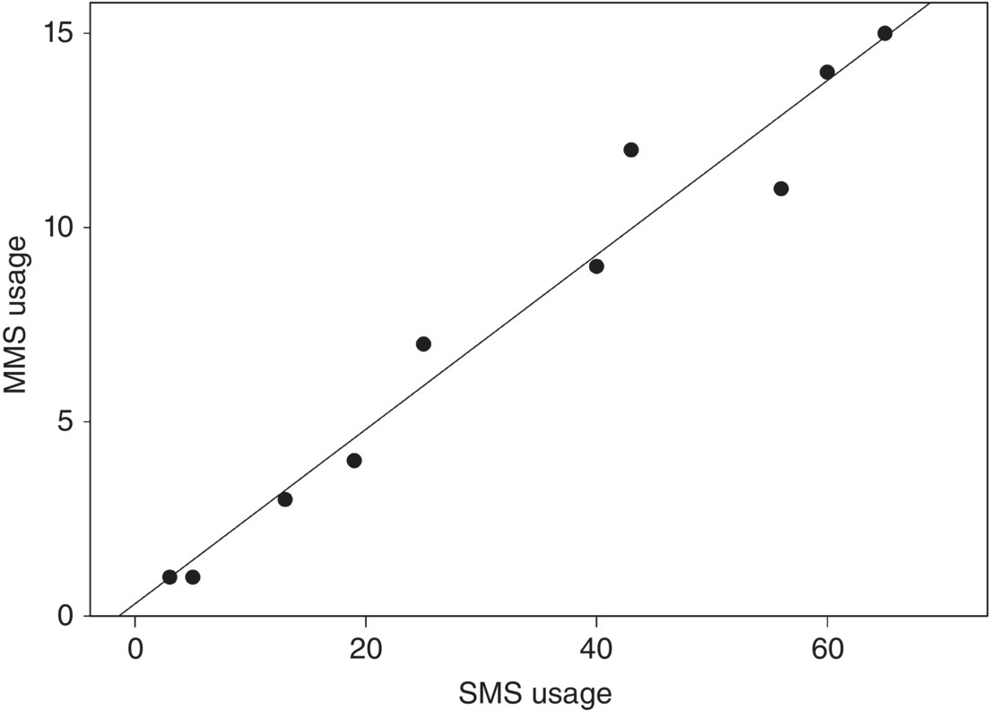
Figure 5.1 Linear correlation between two continuous measures
As seen in the above plot, most customer dots cluster around a straight line with a positive slope that slants upward to the right. Customers with increased sms usage also tend to be mms users as well. These two services are related in a linear manner, and they present a strong, positive linear correlation, since high values of one field tend to correspond with high values of the other. On the other hand, in negative linear correlations, the direction of the relationship is reversed. These relationships are summarized by straight lines with a negative slope that slant downward. In such cases, high values of one field tend to correspond with low values of the other. The strength of linear correlation is quantified by a measure named Pearson correlation coefficient. It ranges from −1 to +1. The sign of the coefficient reveals the direction of the relationship. Values close to +1 denote strong positive correlation while values close to −1 negative correlation. Values around 0 denote no discernable linear correlation, yet this does not exclude the possibility of nonlinear correlation.
So PCA is identifying strong linear relationships between the original inputs, and its goal is to replace them with the smallest number of components that account for as much as possible of their information. Moreover, a typical PCA analysis derives uncorrelated components, appropriate for input in many other modeling techniques, including clustering. The derived components are produced by linear transformations of the inputs, as shown by the following formula:

where Ck denotes the component k produced by the inputs Fi. The n inputs can produce a maximum of n components; however, in practice, the number of components retained is much smaller since the main goal is the reduction of dimensionality.
The coefficients ![]() are calculated by the algorithm so that the loss of information is minimal. The components are extracted in decreasing order of importance with the first one being the most significant as it accounts for the largest amount of input data information. Specifically, the first component is the linear combination that explains as much as possible of the total variability of the input fields. Thus, it retains most of their information. The second component accounts for the largest amount of the unexplained variability, and it is also uncorrelated with the first component. Subsequent components are constructed to account for the remaining information.
are calculated by the algorithm so that the loss of information is minimal. The components are extracted in decreasing order of importance with the first one being the most significant as it accounts for the largest amount of input data information. Specifically, the first component is the linear combination that explains as much as possible of the total variability of the input fields. Thus, it retains most of their information. The second component accounts for the largest amount of the unexplained variability, and it is also uncorrelated with the first component. Subsequent components are constructed to account for the remaining information.
Since n components are required to fully account for the original information of the n fields, the question is where to stop and how many components to extract? Although there are specific technical criteria that can be applied to guide analysts on the procedure, the final decision should also take into account business criteria such as the interpretability and the business meaning of the components. The final solution should balance between simplicity and effectiveness, consisting of a reduced and interpretable set of compound attributes that can sufficiently represent the original fields.
Key issues that a data miner has to face in a PCA analysis include:
- How many components to extract?
- Is the derived solution efficient and useful?
- Which original fields are mostly related with each component?
- What does each component represent? In other words, what is the meaning of each component?
The next paragraphs will try to clarify these issues.
5.2.1 How many components to extract?
In the next paragraphs, we’ll present PCA by examining the fixed telephony usage fields of Table 5.1.
Table 5.1 Behavioral fields used in the PCA example
| Field name | Description |
| FIXED_OUT_CALLS | Monthly average of outgoing calls to fixed telephone lines |
| FIXED_OUT_MINS | Monthly average number of minutes of outgoing calls to fixed telephone lines |
| PRC_FIXED_OUT_CALLS | Percentage of outgoing calls to fixed telephone lines: outgoing calls to fixed lines as a percentage of the total outgoing calls |
| MOBILE_OUT_CALLS | Monthly average of outgoing calls to mobile telephone lines |
| PRC_MOBILE_OUT_CALLS | Percentage of outgoing calls to mobile telephone lines |
| BROADBAND_DAYS | Days with broadband traffic |
| BROADBAND_TRAFFIC | Monthly average broadband traffic |
| INTERNATIONAL_OUT_CALLS | Monthly average of outgoing calls to international telephone lines |
| PRC_INTERNATIONAL_OUT_CALLS | Percentage of outgoing international calls |
Table 5.2 lists the pairwise Pearson correlation coefficients among the original fields.
Table 5.2 Pairwise correlation coefficients among inputs
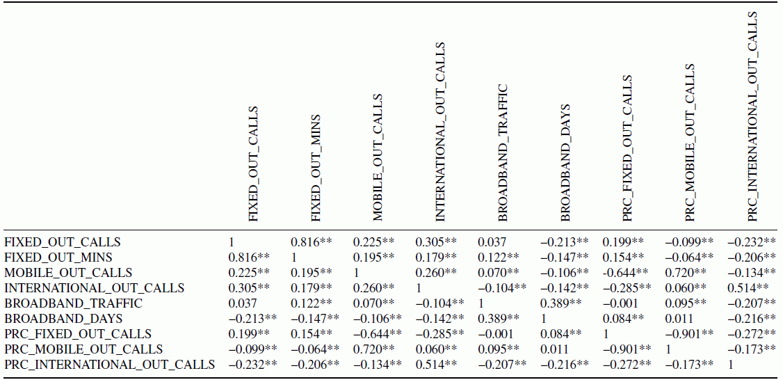
As shown in the table, there are significant correlations among specific usage fields. Statistically significant correlations (at the 0.01 level) are denoted by the symbol “**” The number of outgoing calls to fixed lines, for instance, is positively correlated with the minutes of such calls, denoting that customers that make a large number of voice calls also tend to talk a lot. Other fields are negatively correlated such as the percentage of calls to fixed and mobile lines. This signifies a contrast between calls to fixed and mobile phone numbers, not in terms of usage volume but in terms of the total usage ratio that each service accounts for. Studying correlation tables in order to come up to conclusions is a cumbersome job. That’s where PCA comes in. It analyzes such tables and identifies the groups of related fields.
In order to reach a conclusion on how many components to extract, the following criteria are commonly used:
5.2.1.1 The eigenvalue (or latent root) criterion
The eigenvalue is a measure of the variance that each component accounts for. The eigenvalue criterion is perhaps the most widely used criterion for selecting which components to keep. It is based on the idea that a component should be considered insignificant if it does not perform better than a single input. Each single input contains 1 unit of standardized variance; thus, components with eigenvalues below 1 are not extracted.
Figure 5.2 presents the “Total Variance Explained” part of the Modeler PCA output for the fixed telephony data.

Figure 5.2 The “Total Variance Explained” part of the Modeler PCA output for the fixed telephony data
This table presents the eigenvalues and the percentage of variance/information attributable to each component. The components are listed in the rows of the table. The first 4 first rows of the table correspond to the extracted components. A total of nine components is needed to fully account for the information of the nine original fields. That’s why the table contains nine rows. However, not all these components are retained. The algorithm extracted four of them, based on the eigenvalue criterion that we have specified when we set up the model.
The second column of the table denotes the eigenvalue of each component. Components are extracted in descending order of importance so the first one carries over the largest part of the variance of the original fields. Extraction stops at component 4 since the component 5 has an eigenvalue below the requested threshold of 1.
Eigenvalues can also be expressed in terms of the percentage of the total variance of the original fields. The third column of the table, titled “% of Variance,” denotes the variance proportion attributable to each component, while the next column titled “Cumulative %” denotes the total proportion of variance explained by all the components up to that point. The percentage of the initial variance attributable to the four extracted components is about 85%. Not bad at all, if you consider that by only keeping four of the nine original fields, we lose just a small part of their initial information.
5.2.1.2 The percentage of variance criterion
According to that criterion, the number of components to be extracted is determined by the total explained percentage of variance. The threshold value for extraction depends on the specific situation, but in general, a solution should not fall below 70%.
Figure 5.3 presents the eigenvalues part of the RapidMiner PCA output for the fixed telephony example. Note that the inputs have been normalized with a z-transformation before the model training.
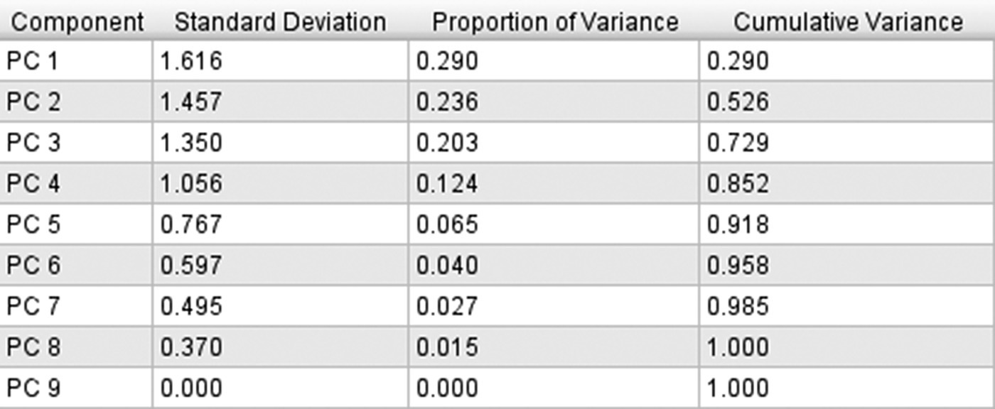
Figure 5.3 The eigenvalues of the RapidMiner PCA model results
The rows of the output table correspond to the derived components. The proportion of variance attributable to each component is displayed in the third column. The cumulative variance explained is listed in the fourth column. Note that these values are equal to the ones produced by the Modeler PCA model. A variance threshold of 85% has been set for the dimensionality reduction. This model setting leads to the retaining of the first four components.
5.2.1.3 The scree test criterion
Eigenvalues decrease in a descending order along with the extracted components. According to that criterion, we should look for a sudden large drop in the eigenvalues which indicate transition from large to small values. At that point, the unique variance (variance attributable to a single field) that a component carries over starts to dominate the common variance. This criterion is graphically illustrated by the scree plot which plots the eigenvalues against the number of extracted components. What we should look for is a steep downward slope of the eigenvalues’ curve followed by a straight line. In other words, the first “bend” or “elbow” that would resemble the scree at the bottom of a mountain. The starting point of the “bend” indicates the maximum number of components to extract while the point immediately before the “bend” could be selected for a more “compact” solution.
5.2.1.4 The interpretability and business meaning of the components
Like any other model, data miners should experiment and try different extraction solutions before reaching a decision. The final solution should include directly interpretable, understandable, and useful components. Since the retained components will be used for subsequent modeling and reporting purposes, analysts should be able to recognize the information that they convey. A component should have a clear business meaning otherwise it would be of little value for further usage. In the next paragraph, we shall present the way to interpret components and to recognize their meaning.
5.2.2 What is the meaning of each component?
The next task is to determine the meaning of the derived components, in respect to the original fields. The goal is to understand the information that they convey and name them accordingly. This interpretation is based on the correlations among the derived components and the original inputs. These correlations are referred to as loadings. In RapidMiner, they are presented in the “Eigenvectors” view of the PCA results.
The rotation is a recommended technique to apply in order to facilitate the components’ interpretation process. The rotation minimizes the number of fields that are strongly correlated with many components and attempts to associate each input with one component. There are numerous rotation techniques, with varimax being the most popular for data reduction purposes since it yields transparent components which are also uncorrelated, a characteristic usually wanted for next tasks. Thus, instead of looking at the original loadings, we typically examine the loadings after the application of a rotation method.
Figure 5.5 presents the rotated component matrix of the Modeler PCA model with varimax rotation. It lists the loadings of the inputs and the components of our example. Note that loadings with absolute values below 0.4 have been suppressed for easier interpretation. Moreover, the original inputs have been sorted according to their loadings so that fields associated with the same component appear together as a set.
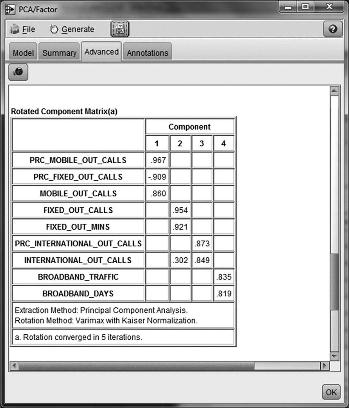
Figure 5.5 The rotated component matrix of the Modeler PCA model for the interpretation of the components
To understand what each component represents, we should identify the original fields with which it is associated and the extent and the direction of this association. Hence, the interpretation process involves the examination of the loading values and their signs and the identification of significant correlations. Typically, correlations above 0.4 in absolute value are considered of practical significance, and they denote the original fields which are representative for each component. The interpretation process ends up with the naming of the derived components with names that appropriately summarize their meaning.
In the fixed telephony example, component 1 seems to be strongly associated with calls to mobile numbers. Both the number (MOBILE_OUT_CALLS) and the ratio of calls to mobile lines (PRC_ MOBILE_OUT_CALLS) load heavily on this component. The negative sign in the loading of the fixed-calls ratio (PRC_FIXED_OUT_CALLS) indicates a strong negative correlation with component 1. It suggests a contrast between calls to fixed and mobile numbers, in terms of usage ratio. We can label this component as “CALLS_TO_MOBILE” as it seems to measure this usage aspect.
The number and minutes of outgoing calls to fixed lines (FIXED_OUT_CALLS and FIXED_OUT_MINS) seem to covary, and they are combined to form the second component which can be named as “CALLS_TO_FIXED.” By examining the loading in a similar way, we can conclude that the component 3 represents “INTERNATIONAL_CALLS” and the component 4 “BROADBAND” usage.
Ideally, each field would heavily load on a single component and the original inputs would be clearly separated into distinct groups. This is not always the case though. Fields that do not load on any of the extracted components or fields not clearly separated are indications of a solution that fails to explain all the original fields. In these cases, the situation could be improved by requesting a richer solution with more extracted components.
5.2.3 Moving along with the component scores
The identified components can be used in the subsequent data mining models, provided of course they comprise a conceptually clear and meaningful representation of the original inputs. The PCA algorithm derives new composite fields, named component scores, that denote the values of each instance in the revealed components. Component scores are produced through linear transformations of the original fields, by using coefficients that correspond to the loading values. They can be used as any other inputs in subsequent tasks.
The derived component scores are continuous numeric fields with standardized values; hence, they have a mean of 0 and a standard deviation of 1, and they designate the deviation from the average behavior. As noted before, the derived component scores, apart from being fewer in number than the original inputs, are standardized and uncorrelated and equally represent all the input dimensions. These characteristics make them perfect candidates for inclusion in subsequent clustering algorithms for segmentation.
@Modeling tech tips
The IBM SPSS Modeler PCA model
Figure 5.6 and Table 5.3 present the parameter settings of the PCA algorithm in IBM SPSS Modeler.

Figure 5.6 The PCA model settings in IBM SPSS Modeler
Table 5.3 The PCA model parameters in IBM SPSS Modeler
| Option | Explanation/effect |
| Extraction method | PCA is the recommended extraction method in cases where data reduction is the first priority |
| Worth trying alternatives: other data reduction algorithms like Principal Axis Factoring and Maximum Likelihood which are the most commonly used factor analysis methods | |
| Extract factors | Sets the criterion for the number of components to be extracted. The most common criterion is based on the eigenvalues: only components with eigenvalues above 1 are retained |
| Worth trying alternatives: analysts can experiment by setting a different threshold value. Alternatively, based on the examined results, they can ask for a specific number of components to be retained through the “maximum number (of factors)” option | |
| Rotation | Applies a rotation method. Varimax rotation can facilitate the interpretation of components by producing clearer loading patterns |
| Sort values | This option aids the interpretation of the components by improving the readability of the rotated component matrix. When selected, it places together the original fields associated with the same component |
| Hide values below | This option aids the component interpretation by improving the readability of the rotated component matrix. When selected, it suppresses loadings with absolute values lower than 0.4 and allows users to focus on significant loadings |
The RapidMiner PCA model
Figure 5.7 and Table 5.4 present the parameter settings of the PCA model in RapidMiner.

Figure 5.7 The PCA model settings in RapidMiner
Table 5.4 The PCA model parameters in RapidMiner
| Option | Explanation/effect |
| Dimensionality reduction | Sets the criterion for the number of components to be retained. The ‘keep variance” option removes the components with a cumulative variance explained greater than the specified threshold. The “fixed number” option keeps the specified number of components |
| Variance threshold (or fixed number) | The “variance threshold” option is invoked with the ‘keep variance” dimensionality reduction criterion. The default threshold is 0.85, and in most cases, it is a good starting point for experimenting. The “fixed number” option allows users to request a specific number of components to be extracted |
5.3 Clustering algorithms
Clustering models are unsupervised techniques, appropriate when there is no target output. They analyze the input data patterns and reveal the natural groupings of records. The groups identified are not known in advance, as is the case in classification modeling. Instead, they are recognized by the algorithms. The instances are assigned to the detected clusters based on their similarities in respect to the inputs.
According to the way they work and their outputs, the clustering algorithms can be categorized in two classes, the hard and the soft clustering algorithms. The hard clustering algorithms, such as K-means, assess the distances (dissimilarities) of the instances. The revealed clusters do not overlap and each instance is assigned to one cluster. The soft clustering techniques on the other hand, such as Expectation Maximization (EM) clustering, use probabilistic measures to assign the instances to clusters with certain probabilities. The clusters can overlap and the instances can belong to more than one cluster with certain, estimated probabilities.
5.3.1 Clustering with K-means
K-means is one of the most popular clustering algorithms. It is a centroid-based partitioning technique. It starts with an initial cluster solution which is updated and adjusted until no further refinement is possible (or until the iterations exceed a specified number). Each iteration refines the solution by increasing the within cluster homogeneity and by reducing the within cluster variation. Although K-means has been traditionally used to cluster numerical inputs, with the use of special distance measures or internal encodings, it can also handle mixed numeric and categorical inputs.
The “means” part of the algorithm’s name refers to the fact that the centroid of each cluster, the cluster center, is defined by the means of the inputs in the cluster. The “K” comes from the fact that analysts have to specify in advance the number of k clusters to be formed. The selection of the number of clusters to be formed can be based on preliminary model training and/or prior business knowledge. A heuristic approach involves building candidate models for a range of different k values (typically between 4 and 15), comparing the obtained solutions in respect to technical measures (such as the within cluster variation or the Bayesian Information Criterion (BIC)) and conclude the best k. Such approaches are followed by Excel’s K-means and RapidMiner’s X-means models. The goal is to balance the trade-off between quality and complexity and produce actionable and homogenous clusters of a manageable number.
K-means uses a distance measure, for instance, the Euclidean distance, and iteratively assigns each record in the derived clusters. It is very quick since it does not need to calculate distances between all the pairs of the records. Clusters are refined through an iterative procedure during which records move between the clusters until the procedure becomes stable. The procedure starts by selecting k well-spaced initial records as cluster centers (initial seeds) and assigns each record to its “nearest” cluster. As new records are added to the clusters, the cluster centers are recalculated to reflect their new members. Then, cases are reassigned to the adjusted clusters. This iterative procedure is repeated until it reaches convergence and the migration of records between the clusters no longer refines the solution.
The K-means procedure is graphically illustrated in Figure 5.8. For easier interpretation, we assume two inputs and the use of the Euclidean distance measure.
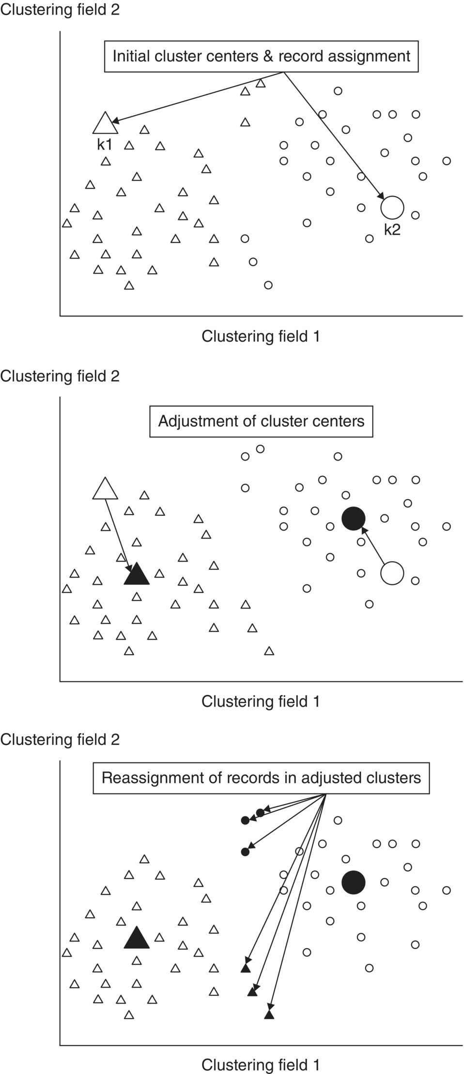
Figure 5.8 An illustration of the K-means clustering process
A drawback of the algorithm is that, at an extent, it depends on the initial selected cluster centers. A recommended approach is to perform multiple runs and train different models, each with a different initialization, then pick the best model. K-means is also sensitive to outliers since cases with extreme values can have a big influence on the cluster centroids. K-medoids, a K-means variant, addresses this drawback by using centroids which are actual data points. Each cluster is represented by an actual data point instead of using the hypothetical instance defined by the cluster means. Each remaining case is then assigned to the cluster with the most similar representative data point, according to the selected distance measure.
On the other hand, K-means advantages include its speed and scalability: it is perhaps the fastest clustering model, and it can efficiently handle long and wide datasets with many records and input clustering fields.
Figure 5.9 presents the distribution of the five clusters revealed by Modeler’s K-means algorithm on the fixed telephony data.

Figure 5.9 The distribution of the five clusters revealed by Modeler’s K-means algorithm on the fixed telephony data
Figure 5.10 presents the centroids of the identified clusters.
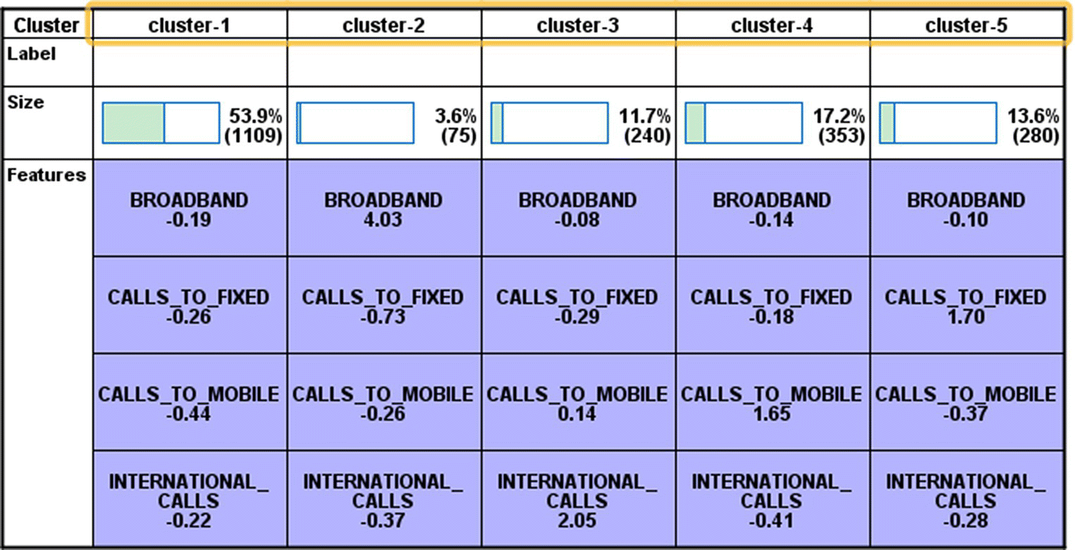
Figure 5.10 The centroids of the fixed telephony clusters
The table of centroids presents the means of each input across clusters. Since in this example the clustering inputs are normalized PCA scores, a mean above or below 0 designates deviation from the mean of the total population. The solution includes a dominant cluster of basic users, the cluster 1. The members of cluster 2 present a high average on the broadband component. Hence, cluster 2 seems to include the heavy internet users. Customers with increased usage of international calls are assigned to cluster 3, while cluster 4 is characterized by increased usage of mobile calls. Finally, cluster 5 is dominated by fixed-calls customers.
The IBM SPSS Modeler K-means cluster
The parameters of the IBM SPSS Modeler K-means algorithm are presented in Figure 5.11 and in Table 5.5.
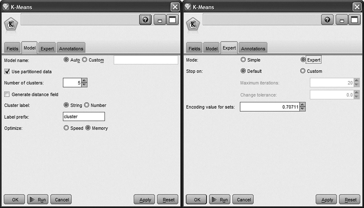
Figure 5.11 IBM SPSS Modeler K-means options
Table 5.5 IBM SPSS Modeler K-means parameters
| Option | Explanation/effect |
| Number of clusters | Users should experiment with different number of clusters to find the one that best fits their specific business goals |
| Worth trying alternatives: users can get an indication on the underlying number of clusters by trying other clustering techniques that incorporate specific criteria to automatically detect the number of clusters | |
| Generate distance field | It generates an additional field denoting the distance of each record to the center of the cluster assigned. It can be used to assess whether a case is a typical representative of its cluster or lies far apart from the rest of the other members |
| Maximum iterations and change tolerance | The algorithm stops if after a data pass (iteration) the cluster centers do not change (0 change tolerance) or after the specified number of iterations have been completed, regardless of the change of the cluster centers. Higher tolerance values lead to faster but most likely worse models |
| Users can examine the solution steps and the change of cluster centers at each iteration. In the case of nonconvergence after the specified number of iterations, they should rerun the algorithm with the number of iterations increased | |
| Encoding value for sets | In K-means, each categorical field is transformed to a series of numeric flags. The default encoding value is the square root of 0.5 (approximately 0.7071 07). Higher values closer to 1.0 will weight categorical fields more heavily |
The RapidMiner K-means and K-medoids cluster
The parameters of RapidMiner’s K-means and K-medoid models are presented in Figure 5.12 and in Table 5.6.
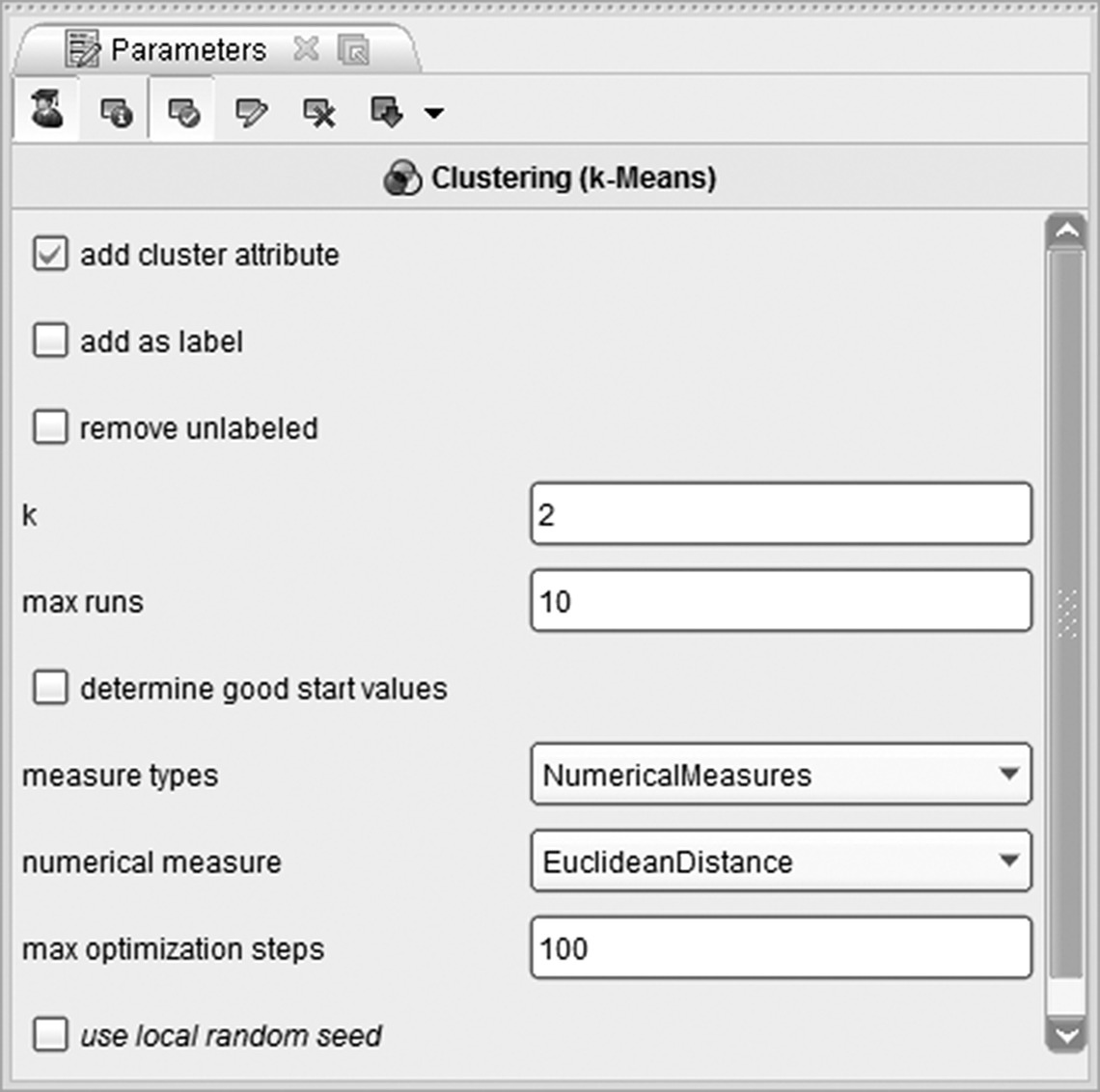
Figure 5.12 RapidMiner’s K-means options
Table 5.6 RapidMiner’s K-means and K-medoid parameters
| Option | Explanation/effect |
| Add cluster attribute | Adds a cluster membership field. By default is selected |
| Add as label | When checked, the cluster attribute field is assigned a label (target) role instead of a cluster role |
| Remove unlabeled | When on, records not assigned to a cluster are deleted |
| k | Specifies the number of clusters to be formed |
| Determine good start values (for K-means) | A recommended option for K-means cluster which ensures that k well-spaced records are chosen as the start centroids for the algorithm |
| Max runs/max optimization steps | The “max optimization steps” option specifies the maximum number of optimization iterations for each run of the algorithm. The “max runs” option sets the maximum number of different times the algorithm will run. At each run, different random start centroids are used in order to decrease the dependency of the solution to the starting points |
| Measure types and measure | The combination of these two options sets the measure type and the measure which will be used to assess the similarities of records. The selection depends on the type and the measurement level of the inputs but as always, experimentation with different distance measures and number of clusters should be done. The available numerical measures include the classic Euclidean distance and other measures such as the Chebyshev and the Manhattan distances. The class of nominal measures includes the Dice similarity and others. The mixed Euclidean distance is included in the class of mixed measures, appropriate in the case of mixed inputs. Finally, the squared Euclidean distance as well as other measures such as the KL divergence and Mahalanobis distance are available in the class of Bregman divergences (distances) |
| (Use) local random seed | By specifying a local random seed, we “stabilize” the random selection of the initial cluster centroids, ensuring that the same clustering results can be reproduced |
Clustering in Data Mining for Excel
The parameters of the Data Mining for Excel Cluster are presented in Figure 5.13 and discussed in Table 5.7.
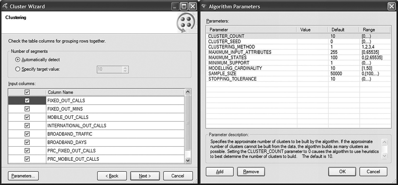
Figure 5.13 The cluster options of Data Mining for Excel
Table 5.7 The cluster parameters of Data Mining for Excel
| Option | Explanation/effect |
| Number of segments | In the clustering step of the Cluster wizard, apart from the clustering inputs, analysts specify the number of clusters to be formed. They can specify a specific target value based on prior experimentation or they can let the algorithm use heuristics to autodetect the optimal number of clusters. In the heuristic procedure, many models are trained on a small sample of data and compared based on fit measures to find the optimal number of clusters |
| Cluster count | The “number of segments choice” made in the Clustering wizard is inherited in the “Cluster count” parameter. If the specified number of clusters cannot be built from the data, the algorithm builds as many clusters as possible. A value of 0 in the “Cluster count” parameter invokes autodetection of clusters |
| Cluster seed | By specifying a random seed, we “stabilize” the random sampling done in the initial steps of the algorithm, ensuring that the same clustering results can be reproduced |
| Clustering method | Available methods include scalable Expectation Maximization (EM), nonscalable EM, scalable K-means, and nonscalable K-means Scalable methods are based on sampling to address performance issues in the case of large datasets. Nonscalable methods (K-means and EM) load and analyze the entire dataset in one clustering pass. On the other hand, scalable methods use a sample of cases (the default sample size is 50 000 cases) and load more cases only if the model has not converged and it is necessary to improve its fit. Nonscalable methods might produce slightly more accurate solutions but are demanding in terms of process time and resources. In the case of large datasets, the scalable methods are recommended |
| Sample size | Sets the sample size of each data pass for the scalable clustering methods The default value is 50 000 |
| Maximum input attributes | A threshold parameter for the integrated feature selection preprocessing step. Feature selection is invoked if the number of inputs is greater than the specified value |
| A value of 0 turns off feature selection. The default value is 255 | |
| Maximum states | This option determines the maximum number of input categories (“states”) that the algorithm will analyze. If an attribute has more categories than the specified threshold, then only the most frequent categories will be used and the remaining and rare categories are treated as missing |
| The default value is 100 | |
| Minimum support | This option sets the minimum allowable number of cases in each detected cluster. If the number of cases in a cluster is lower than the specified threshold, the cluster is treated as empty, discarded, and reinitialized |
| The default value of 1 in almost all cases should be altered with a higher value | |
| Modeling cardinality | Controls the number of runs, the number of different candidate models that are built during the clustering process. Each model is built with a different random initialization to decrease the dependency of the solution to the starting points. Finally, the best model of the candidates is picked. Lower values improve speed, since fewer candidate models are built, but also increase the risk of a lower-quality solution |
| The default value is 100 | |
| Stopping tolerance | Specifies the accepted tolerance for stopping the model training. The model stops and convergence is reached when the overall change in cluster centers or the overall change in cluster probabilities is less than the ratio of the specified “Stopping Tolerance” parameter divided by the number of the clusters |
| The default value is 10. Higher tolerance values lead to faster but riskier models |
5.3.2 Clustering with TwoStep
TwoStep is a scalable clustering model, based on the BIRCH algorithm, available in IBM SPSS Modeler that can efficiently handle large datasets. It uses a log-likelihood distance measure to accommodate mixed, continuous, and categorical inputs.
Unlike classic hierarchical techniques, it performs well with big data due to the initial resizing of the input records to subclusters. As the name implies, the clustering process is carried out in two steps. In the first step of preclustering, the entire dataset is scanned and a clustering feature tree (CF tree) is built, comprised by a large number of small preclusters (“microclusters”). Instead of using the detailed information of its member instances to characterize each precluster, summary statistics are used such as the centroid (mean of inputs), radius (average distance of member cases to the centroid), and diameter (average pairwise distance within the precluster) of the preclusters. Each case is recursively guided to its closest precluster. If the respective distance is below an accepted threshold, it is assigned to the precluster. Otherwise, it starts a precluster of its own. In the second phase of the process, an hierarchical (agglomerative) clustering algorithm is applied to the CF tree preclusters which are recursively merged until the final solution.
TwoStep uses heuristics to suggest the optimal number of clusters by taking into account:
- The goodness of fit of the solution. The Bayesian Information Criterion (BIC) or the Akaike Information Criterion (AIC) measure is used to assess how well the specific data are fit by the current number of clusters.
- The distance measure for merging the preclusters. The algorithm examines the final steps of the hierarchical procedure and tries to spot a sudden increase in the merging distances. This point indicates that the agglomerative procedure has started to join dissimilar clusters, and hence, it indicates the correct number of clusters to fit.
Another TwoStep advantage is that it integrates an outlier handling option that minimizes the effects of noisy records which could otherwise distort the segmentation solution. Outlier identification is taking place in the preclustering phase. Sparse preclusters with few members compared to other preclusters (less than 25% of the largest precluster) are considered as potential outliers. These outlier cases are set aside and the preclustering procedure is rerun without them. Outliers that still cannot fit the revised precluster solution are filtered out from the next step of hierarchical clustering, and they do not participate in the formation of the final clusters. Instead, they are assigned to a “noise” cluster.
The algorithm is fast and scalable; however, it seems to work best when the clusters are spherical in shape.
@Modeling tech tips
The IBM SPSS Modeler TwoStep cluster
The IBM SPSS Modeler TwoStep cluster options are listed in Figure 5.14 and Table 5.8.

Figure 5.14 The IBM SPSS Modeler TwoStep cluster options
Table 5.8 The IBM SPSS Modeler TwoStep cluster parameters
| Option | Explanation/effect |
| Standardize numeric fields | By default, the numeric inputs are standardized in the same scale (mean and standard deviation of 1) |
| Automatically calculate number of clusters | This option invokes autoclustering and lets the algorithm suggest the number of clusters to fit. The “Maximum” and “Minimum” text box values define the range of solutions that will be evaluated. The default setting limits the algorithm to evaluate the last 15 steps of the hierarchical clustering procedure and to propose a solution comprising from a minimum of 2 up to a maximum of 15 clusters |
| The autoclustering option is the typical approach for starting the model training. Alternatively, analysts can set a specific number of clusters to be created through the Specify number of clusters option | |
| Exclude outliers | When selected, handling of outliers is applied, an option generally recommended as it tends to yield richer clustering solutions |
| Distance measure | Sets the distance measure to be used for assessing the similarities of cases. Available measures include the log-likelihood (default) and the Euclidean distance. The latter can be used only when the inputs are continuous |
| Clustering criterion | Sets the criterion to be used in the autoclustering process to identify the optimal number of clusters. The criteria include the Bayesian Information Criterion (BIC) and the Akaike Information Criterion (AIC) |
5.4 Summary
Clustering techniques are applied for unsupervised segmentation. They find natural groupings of records/customers with similar characteristics. The revealed clusters are directed by the data and not by subjective and predefined business opinions. There are not right or wrong clustering solutions. The value of each solution depends on its ability to represent transparent, meaningful, and actionable customer typologies.
In this chapter, we’ve presented only some of the available clustering techniques: K-means and K-medoids and the TwoStep cluster model based on the BIRCH algorithm. We’ve also dedicated a part of the chapter to PCA analysis. Although not required, PCA is a recommended data preparation step as it reduces the dimensionality of the inputs and identifies the distinct behavioral aspects to be used for unbiased segmentation.