
8
Segmentation application in telecommunications
8.1 Mobile telephony: the business background and objective
In an environment of hard competition, especially in the case of mature markets, offering of high-level quality services is essential for mobile phone network operators to become established in the market. In times of rapid changes and hard competition, focusing only on customer acquisition, which is nevertheless becoming more and more difficult, is not enough. Inevitably, organizations have to also work on customer retention and on gaining a larger “share of customer” instead of only trying to gain a bigger slice of the market. Growth from within is sometimes easier to achieve and equally important as winning customers from competitors.
Hence, keeping customers satisfied and profitable is a one way street for success. In order to achieve this, operators have to focus on customers and understand their needs, behaviors, and preferences. Behavioral segmentation can help in the identification of the different customer typologies and in the development of targeted marketing strategies.
Nowadays, customers may choose from a huge variety of offered services. The days of voice-only calls are long gone. Mobile phones are communication centers and it’s up to the user to select the way of usage that suits his needs. People can communicate via SMS and MMS messages. They can use their phones for connecting to the Internet, for sending e-mails, for downloading games and ringtones, and for communicating with friends and family when they travel abroad. Mobile phones are perceived differently by various people. Some customers only use them in rare circumstances and mainly for receiving incoming calls. Others are addicted to their devices and cannot live without them. Some treat them as electronic gadgets, while for others, they are a tool for work.
As you can imagine, this multitude of potential choices results in different usage patterns and typologies. Once again, the good news is that usage is recorded in detail. Call Detail Records (CDRs) are stored, providing a detailed record of usage. They contain detailed information about all types of calls made. When aggregated and appropriately processed, they can provide valuable information for behavioral analysis.
All usage history should be stored in the organization’s mining datamart. Information about frequency and intensity of usage for each call type (voice, SMS, MMS, Internet connection, etc.) should be taken into account when trying to identify the different behavioral patterns. In addition to this, information such as the day/time of the calls (workdays vs. nonworkdays, peak vs. off-peak hours, etc.), roaming usage, direction of calls (incoming vs. outgoing), and origination/destination network type (on-net, off-net, etc.) could also contribute in the formation of a rich segmentation solution.
In this section, we’ll present a segmentation example from the mobile telephony market. Marketers of a mobile phone network operator decided to segment their customers according to their behavior. They used all the available usage data to reveal the natural groupings in their customer base. Their goal was to fully understand their customers in order to:
- Develop tailored sales and marketing strategies for each segment.
- Identify distinct customer needs and habits and proceed to the development of new products and services, targeting the diverse usage profiles of their customers. This could directly lead to increased usage on behalf of existing customers but might also attract new customers from the competition.
8.2 The segmentation procedure
The methodological approach followed was analogous to the general framework presented in detail in the relevant chapter. In this section, we’ll just present some crucial points concerning the project’s implementation plan, which obviously affected the whole application. The key step of the process was the application of a cluster model to segment the consumer postpaid customer base according to their behavioral similarities. The application of the clustering algorithm was preceded by a data reduction technique which identified the underlying data dimensions which were used as inputs for clustering. The entire procedure is described in detail in the following paragraphs.
8.2.1 Selecting the segmentation population: the mobile telephony core segments
Mobile telephony customers are typically categorized in core segments according to their rate plans and the type of the relationship with the operator. The first segmentation level differentiates residential (consumer) from business customers. Residential customers are further divided into postpaid and prepaid:
- Postpaid—contractual customers: Customers with mobile phone contracts. Usually, they comprise the majority of the customer base. These customers have a contract and a long-term billing arrangement with the network operator for the received services. They are billed on a monthly basis and according to the traffic of the past month; hence, they have unlimited credit.
- Prepaid customers: They do not have a contract-based relationship with the operator, and they are buying credit in advance. They do not have ongoing billing and they pay for the services before actually using them.
Additionally, business customers are further differentiated according to their size into corporate, SME, and SOHO customers.
The typical core segments in mobile telephony are depicted in Figure 8.1.
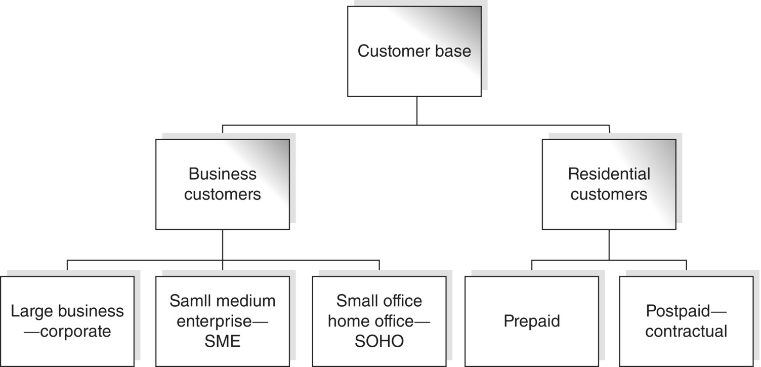
Figure 8.1 Core segments in mobile telephony.
Source: Tsiptsis and Chorianopoulos (2009). Reproduced with permission from Wiley
The objective of the marketers was to enrich the core segmentation scheme with refined subsegments. Therefore, they decided to focus their initial segmentation attempts exclusively on residential postpaid customers. Prepaid customers need a special approach in which attributes like the intensity and frequency of top-ups (recharging of their credits) should also be taken into account. Business customers also need a different handling since they comprise a completely different market. It is much safer to analyze those customers separately, with segmentation approaches such as value based, size based, industry based, etc.
Moreover, only MSIDNs (telephone numbers) with current status active or in suspension (due to payment delays) were included in the analysis. Churned (voluntary and involuntary churners) MSISDNs have been excluded from the start. Their “contribution” is crucial in the building of a churn model but trivial in a segmentation scheme mainly involving phone usage. In addition, segmentation population was narrowed down even further by excluding users with no incoming or outgoing usage within the past 6 months. Those users have been flagged as inactive, and they have been selected for further examination and profiling. They could also form a target list for an upcoming reactivation campaign, but they do not have much to contribute to a behavioral analysis since, unfortunately, inactivity is their only behavior at the moment.
8.2.2 Deciding the segmentation level
Customers may own more than one MSISDN which may use in a different manner to cover different needs. In order to capture all the potentially different usage behaviors of each customer, it has been decided to implement the behavioral segmentation at MSISDN level. Therefore, relevant input data have been preaggregated accordingly, and the derived cluster model assigned each MSISDN to a distinct behavioral segment.
8.2.3 Selecting the segmentation dimensions
Once again, the mining datamart tables, comprised the main sources of the input data. Table 8.1 outlines the main usage aspects that were selected as segmentation criteria.
Table 8.1 Mobile telephony usage aspects that were investigated in the behavioral segmentation
| Number of calls | Information by Core service type | Voice |
| SMS | ||
| MMS | ||
| Internet | ||
| … | ||
| Minutes/traffic Community | Information by Call direction | Incoming |
| Outgoing | ||
| International | ||
| Roaming | ||
The modeling phase was followed by extensive profiling of the revealed segments. In this phase, all available information, including demographic data and contract information details, were cross-examined with the identified customer groups.
8.2.4 Time frames and historical information analyzed
A 6-month observation period was analyzed, a time span that in general ensures the capturing of stable, nonvolatile behavioral patterns instead of random or outdated ones. Summary fields (sums, counts, percentages, averages, etc.) covering the 6-month observation period were used as inputs in the clustering model.
8.3 The data preparation procedure
Readers not interested in the data preparation procedure might skip the following paragraphs and proceed directly to Section 8.4. Note that the data preparation phase presented here is simplified and deals merely with the derivation of KPIs. The Modeler stream for the enrichment of the modeling file with derived KPIs is shown in Figure 8.2. A set of fields, with a PRC_ prefix, was constructed to summarize the relative usage (percentage of total calls) by service type, preferred day/time, as well as the international and the roaming usage. Additionally, the average call duration, both incoming and outgoing, was calculated as the ratio of minutes to number of calls (fields ACD_IN and ACD_OUT, respectively) for each MSISDN.
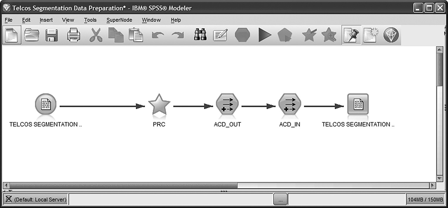
Figure 8.2 The data preparation Modeler stream
8.4 The data dictionary and the segmentation fields
The list of candidate inputs for behavioral segmentation initially included all usage fields contained in the mining datamart and the customer “signature” reference file. In a later stage and according to the organization’s specific segmentation objectives, marketers selected a subset list of clustering inputs which are designated in the last column of Table 8.2.
Table 8.2 Mobile telephony segmentation fields
| Data file: TELCOS SEGMENTATION MODELING DATA.txt | ||
| Field name | Description | Role in the model |
| Community | ||
| OUT_COMMUNITY_TOTAL | Total outgoing community: monthly average of distinct phone numbers that the holder called (includes all call types) | INPUT |
| OUT_COMMUNITY_VOICE | Outgoing voice community | INPUT |
| OUT_COMMUNITY_SMS | Outgoing SMS community | INPUT |
| IN_COMMUNITY_VOICE | Incoming voice community | |
| IN_COMMUNITY_SMS | Incoming SMS community | |
| IN_COMMUNITY_TOTAL | Total incoming community | |
| Number of calls by call type | ||
| VOICE_OUT_CALLS | Monthly average of outgoing voice calls. Derived as the ratio of total voice calls during the 6-month period examined to 6 (months) or to customer tenure for new customers | INPUT |
| VOICE_IN_CALLS | Monthly average of incoming voice calls | INPUT |
| SMS_OUT_CALLS | Monthly average of outgoing SMS calls | INPUT |
| SMS_IN_CALLS | Monthly average of incoming SMS calls | INPUT |
| MMS_OUT_CALLS | Monthly average of outgoing MMS calls | INPUT |
| EVENTS_CALLS | Monthly average of event calls | INPUT |
| INTERNET_CALLS | Monthly average of Internet calls | INPUT |
| TOTAL_OUT_CALLS | Monthly average of outgoing calls (includes all call types) | INPUT |
| Minutes/traffic by call type | ||
| VOICE_OUT_MINS | Monthly average number of minutes of outgoing voice calls | INPUT |
| VOICE_IN_MINS | Monthly average number of minutes of incoming voice calls | INPUT |
| EVENTS_TRAFFIC | Monthly average of events traffic | INPUT |
| GPRS_TRAFFIC | Monthly average of GPRS traffic | INPUT |
| International calls/roaming usage | ||
| OUT_CALLS_ROAMING | Monthly average of outgoing roaming calls (calls made in a foreign country) | INPUT |
| OUT_MINS_ROAMING | Monthly average number of minutes of outgoing voice roaming calls | INPUT |
| OUT_CALLS_INTERNATIONAL | Monthly average of outgoing calls to international numbers (calls made in home country to international numbers) | INPUT |
| OUT_MINS_INTERNATIONAL | Monthly average number of minutes of outgoing voice calls to international numbers | INPUT |
| Usage by day/hour | ||
| OUT_CALLS_PEAK | Monthly average of outgoing calls in peak hours | |
| OUT_CALLS_OFFPEAK | Monthly average of outgoing calls in off-peak hours | |
| OUT_CALLS_WORK | Monthly average of outgoing calls on workdays | |
| OUT_CALLS_NONWORK | Monthly average of outgoing calls on nonworkdays | |
| IN_CALLS_PEAK | Monthly average of incoming calls in peak hours | |
| IN_CALLS_OFFPEAK | Monthly average of incoming calls in off-peak hours | |
| IN_CALLS_WORK | Monthly average of incoming calls on workdays | |
| IN_CALLS_NONWORK | Monthly average of incoming calls on nonworkdays | |
| Days with usage | ||
| DAYS_OUT | Monthly average number of days with any outgoing usage | INPUT |
| DAYS_IN | Monthly average number of days with any incoming usage | INPUT |
| Average call duration | ||
| ACD_OUT | Average duration of outgoing voice calls (in minutes) | INPUT |
| ACD_IN | Average duration of incoming voice calls (in minutes) | INPUT |
| Demographics—profiling fields | ||
| AGE | Age of customer | |
| Gender | Gender of customer | |
| Derived fields (IBM Modeler stream: “Telcos Segmentation Data Preparation.str”) | ||
| PRC_OUT_COMMUNITY_VOICE | Percentage of outgoing voice community: outgoing voice community as a percentage of total outgoing community | INPUT |
| PRC_OUT_COMMUNITY_SMS | Percentage of outgoing SMS community | INPUT |
| PRC_IN_COMMUNITY_VOICE | Percentage of incoming voice community | |
| PRC_IN_COMMUNITY_SMS | Percentage of incoming SMS community | |
| PRC_VOICE_OUT_CALLS | Percentage of outgoing voice calls: outgoing voice calls as a percentage of total outgoing calls | INPUT |
| PRC_SMS_OUT_CALLS | Percentage of SMS calls | INPUT |
| PRC_MMS_OUT_CALLS | Percentage of MMS calls | INPUT |
| PRC_EVENTS_CALLS | Percentage of Event calls | INPUT |
| PRC_INTERNET_CALLS | Percentage of Internet calls | INPUT |
| PRC_OUT_CALLS_ROAMING | Percentage of outgoing roaming calls: roaming calls as a percentage of total outgoing calls | INPUT |
| PRC_OUT_CALLS_INTERNATIONAL | Percentage of outgoing international calls: outgoing international calls as a percentage of total outgoing calls | INPUT |
| PRC_OUT_CALLS_PEAK | Percentage of outgoing calls in peak hours | |
| PRC_OUT_CALLS_OFFPEAK | Percentage of outgoing calls in nonpeak hours | |
| PRC_OUT_CALLS_WORK | Percentage of outgoing calls on workdays | |
| PRC_OUT_CALLS_NONWORK | Percentage of outgoing calls on nonworkdays | |
| PRC_IN_CALLS_PEAK | Percentage of incoming calls in peak hours | |
| PRC_IN_CALLS_OFFPEAK | Percentage of incoming calls in nonpeak hours | |
| PRC_IN_CALLS_WORK | Percentage of incoming calls on workdays | |
| PRC_IN_CALLS_NONWORK | Percentage of incoming calls on nonworkdays | |
Obviously, this list can’t be considered a silver-bullet approach that can cover all the needs of every organization. It represents the approach adopted in the specific implementation but it also outlines a general framework of potential types of fields that could be proved useful in similar applications.
The selected fields indicate the marketers’ orientation to a segmentation scheme that would reflect usage differences in terms of preferred type of calls (voice, SMS, MMS, Internet, etc.), roaming usage (calls made in a foreign country), and frequency of international calls (calls made in home country to international numbers).
The full attribute list of the modeling file is presented in Table 8.2. The last section of the table lists attributes derived through the data preparation phase. The role of each attribute is designated in the last column of the table. Attributes used as inputs in the subsequent models are flagged with an INPUT role.
8.5 The modeling procedure
The IBM SPSS Modeler stream (procedure) for segmentation through clustering is displayed in Figure 8.3. This stream uses the modeling file presented in Table 8.2.
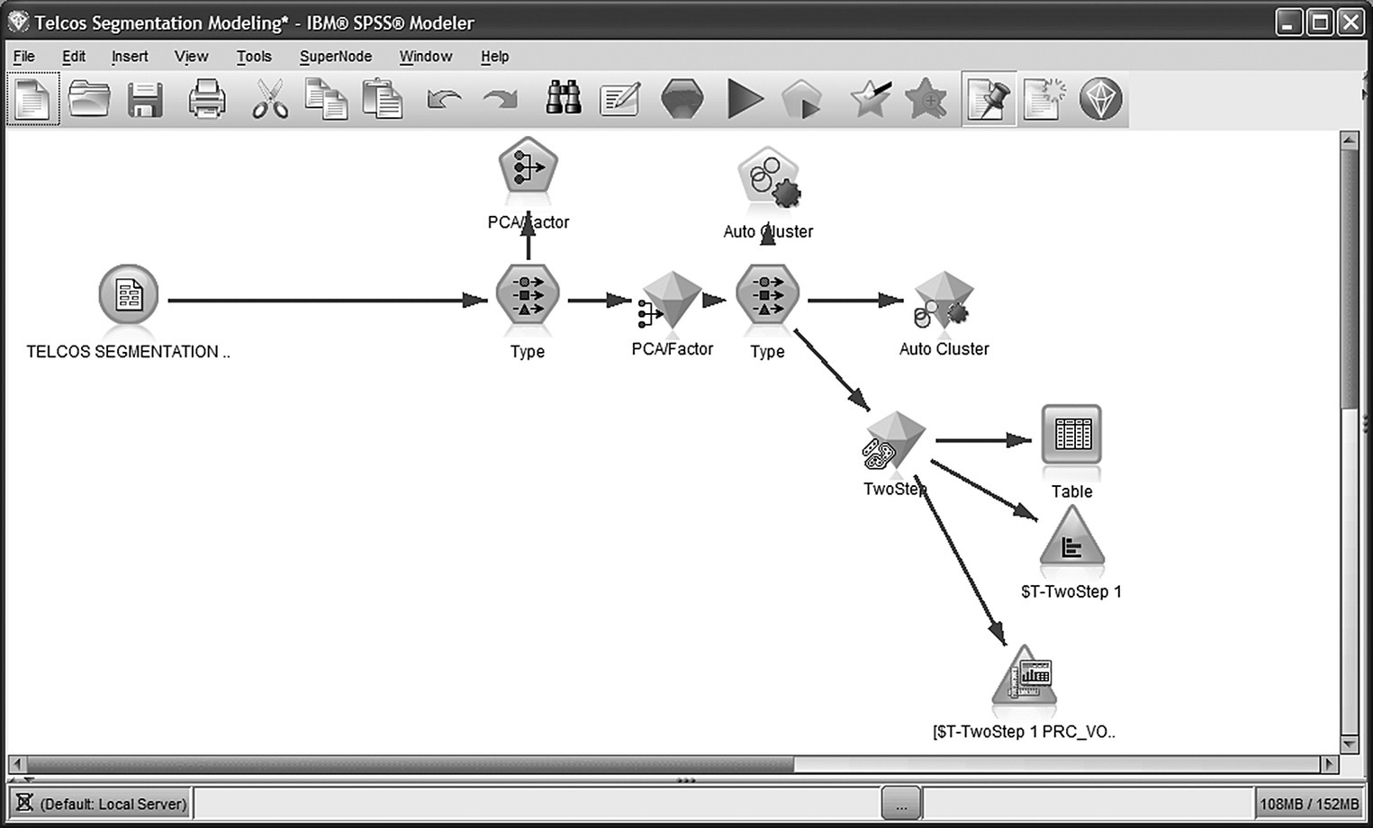
Figure 8.3 The IBM SPSS Modeler procedure for segmentation through clustering
The main modeling steps included:
- The application of a data reduction technique, PCA in particular, to reveal the distinct dimensions of information which were then used as clustering fields
- The use of a cluster model which analyzed the data components identified by PCA and grouped MSISDNs in clusters of similar behaviors
- The profiling of the revealed segments
These steps are explained in detail in the following text.
8.5.1 Preparing data for clustering: combining fields into data components
The number of the original segmentation inputs exceeded 30. Using all those fields as direct input in a clustering algorithm would have produced a complicated solution. Therefore, the approach followed was to incorporate a data reduction technique in order to reveal the underlying data dimensions prior to clustering.
This approach was adopted to eliminate the risk of deriving a biased solution due to correlated attributes. Moreover, it also ensures a balanced solution, in which all data dimensions contribute equally, and it simplifies the tedious procedure of segmentation understanding by providing conceptual clarity.
Specifically, a Principal Components Analysis (PCA) model with varimax rotation was applied to the original segmentation fields. A Type node was used to set as Inputs (Direction In) the designated attributes of Table 8.2. The rest of the attributes were assigned with a None role and didn’t contribute to the subsequent model. The modeling data were then fed into a PCA/Factor modeling node, and a PCA model was developed which grouped original inputs into components. The parameter settings for the PCA model are listed in Table 8.3.
Table 8.3 The PCA model parameter settings
| PCA model parameter settings | |
| Parameter | Setting |
| Model | Principal Components analysis (PCA) |
| Rotation | Varimax |
| Criteria for the number of factors to extract | Initially eigenvalues over 1. Then set to eight components after examination of the results |
Initially, based on the eigenvalues over 1 criterion, the algorithm suggested the extraction of nine components. However, the ninth component was mainly related with a single original attribute, the GPRS traffic. Moreover, it accounted for a small percentage of the information of the original inputs, about 3%. Having considered that, the analysts decided to go for a simpler solution of eight components, selecting to sacrifice a small part of the original information for simplicity. In the eight-component solution, the GPRS traffic was combined with Events usage to form a single component.
Before using the derived components and substituting more than 30 fields with a handful of new ones, the data miners of the organization wanted to be sure that:
- The PCA solution carried over most of the original information.
- The derived components, which would substitute the original attributes, were interpretable and had a business meaning.
Therefore, they started the examination of the model results by looking at the table of “Explained Variance.” Table 8.4 presents these results.
Table 8.4 Deciding the number of extracted components by examining the variance explained table
| Total variance explained | |||
| Components | Eigenvalue | % of variance | Cumulative % |
| 1 | 6.689 | 21.576 | 21.576 |
| 2 | 4.000 | 12.903 | 34.479 |
| 3 | 2.550 | 8.227 | 42.705 |
| 4 | 2.443 | 7.881 | 50.587 |
| 5 | 1.962 | 6.329 | 56.916 |
| 6 | 1.791 | 5.779 | 62.695 |
| 7 | 1.742 | 5.618 | 68.313 |
| 8 | 1.662 | 5.362 | 73.675 |
| 9 | |||
| 10 | |||
| 11 | |||
| … | … | … | … |
| 31 | 0.002 | 0.00 | 100.00 |
The resulted eight components retained more than 73% of the variance of the original fields. This percentage was considered satisfactory and thus the only task left before accepting the components was their interpretation. In practice, only a solution comprised of meaningful components should be retained.
So what do those new composite fields represent? What business meaning do they convey? As these new fields are constructed in order to substitute the original fields in the next stages of the segmentation procedure, it is necessary to be thoroughly decoded before being used in upcoming models.
The component interpretation phase included the examination of the “rotated component matrix” (Table 8.5), a table that summarizes the correlations (loadings) between the components and the original fields.
Table 8.5 Understanding and labeling the components through rotated component matrix
| Rotated component matrix | ||||||||
| Components | ||||||||
| 1 | 2 | 3 | 4 | 5 | 6 | 7 | 8 | |
| OUT_COMMUNITY_TOTAL | 0.918 | |||||||
| OUT_COMMUNITY_VOICE | 0.916 | |||||||
| TOTAL_OUT_CALLS | 0.912 | |||||||
| VOICE_OUT_CALLS | 0.908 | |||||||
| VOICE_IN_CALLS | 0.844 | |||||||
| VOICE_IN_MINS | 0.769 | |||||||
| DAYS_OUT | 0.740 | |||||||
| DAYS_IN | 0.688 | |||||||
| VOICE_OUT_MINS | 0.648 | 0.536 | ||||||
| PRC_OUT_COMMUNITY_SMS | 0.913 | |||||||
| PRC_SMS_OUT_CALLS | 0.903 | |||||||
| PRC_VOICE_OUT_CALLS | −0.822 | |||||||
| OUT_COMMUNITY_SMS | 0.415 | 0.758 | ||||||
| PRC_OUT_COMMUNITY_VOICE | −0.710 | |||||||
| SMS_OUT_CALLS | 0.356 | 0.690 | ||||||
| OUT_CALLS_INTERNATIONAL | 0.907 | |||||||
| OUT_MINS_INTERNATIONAL | 0.894 | |||||||
| PRC_OUT_CALLS_INTERNATIONAL | 0.857 | |||||||
| OUT_MINS_ROAMING | 0.883 | |||||||
| OUT_CALLS_ROAMING | 0.875 | |||||||
| PRC_OUT_CALLS_ROAMING | 0.813 | |||||||
| EVENTS_CALLS | 0.903 | |||||||
| PRC_EVENTS_CALLS | 0.879 | |||||||
| EVENTS_TRAFFIC | 0.447 | |||||||
| GPRS_TRAFFIC | 0.364 | |||||||
| PRC_INTERNET_CALLS | 0.921 | |||||||
| INTERNET_CALLS | 0.903 | |||||||
| PRC_MMS_OUT_CALLS | 0.923 | |||||||
| MMS_OUT_CALLS | 0.918 | |||||||
| ACD_OUT | 0.840 | |||||||
| ACD_IN | 0.683 | |||||||
The “interpretation” results are summarized in Table 8.6.
Table 8.6 The interpretation and labeling of the derived components
| Derived components | |
| Component | Label and description |
| 1 | Voice calls |
| The high loadings in the first column of the rotated component matrix denote a strong positive correlation between Component 1 and the original fields which measure voice usage and traffic such as the number and minutes of outgoing and incoming voice calls (VOICE_OUT_CALLS, VOICE_IN_CALLS, VOICE_OUT_MINS, VOICE_IN_MINS) and the size of the voice community (OUT_COMMUNITY_VOICE). Thus, Component 1 seems to be associated with voice usage | |
| Because generally voice calls constitute the majority of calls for most users and they tend to dominate the total usage, a set of fields associated with total usage (total number of calls, TOTAL_OUT_CALLS) as well as days with usage (DAYS_IN, DAYS_OUT) are also loaded high on this component | |
| 2 | SMS calls |
| Component 2 seems to measure SMS usage and community since it is seems strongly correlated with the percentage of SMS out calls (PRC_SMS_OUT_CALLS) and SMS community (PRC_OUT_COMMUNITY_SMS) | |
| The rather interesting negative correlation between Component 2 and the percentage of voice out calls (PRC_VOICE_OUT_CALLS) denotes a contrast between voice and SMS usage. Thus, users with high positive values in this component are expected to have increased SMS usage and increased SMS to voice calls ratio. This does not necessarily mean low voice traffic, but it certainly implies relatively lower percentage of voice calls and increased percentage of SMS calls | |
| 3 | International calls |
| Component 3 is associated with calls to international networks | |
| 4 | Roaming usage |
| Component 4 seems to measure outgoing roaming usage (making calls when abroad) | |
| 5 | Events and GPRS |
| Component 5 measures Event calls and traffic. GPRS traffic (originally constituting a separate component) is also loaded moderately high on this component | |
| 6 | Internet usage |
| Component 6 is associated with Internet usage | |
| 7 | MMS usage |
| MMS usage seems to be measured by Component 7 | |
| 8 | Average call duration (ACD) |
| Fields denoting average call duration of incoming and outgoing voice calls seem to be related, and they are combined to form Component 8. Unsurprisingly, this component is also associated with minutes of calls (VOICE_OUT_MINS) | |
The explained and labeled components and the respective component scores were subsequently used as inputs in the clustering model. This brings us to the next phase of the application: the identification of useful groupings through clustering.
8.5.2 Identifying the segments with a cluster model
The generated components represented effectively all the usage dimensions of interest, in a concise and comprehensive way, leaving no room for misunderstandings about their business meaning. The next step of the segmentation project included the usage of the derived component scores as inputs in a cluster model. Through a new Type node, the generated components were set as Inputs for the training of the subsequent cluster model.
The clustering process involved the application of an Auto Cluster node for the training and evaluation of 2 TwoStep models with different parameter settings in terms of outlier handling. Figure 8.4 presents an initial comparison of the two cluster models provided by the generated Auto Cluster model.
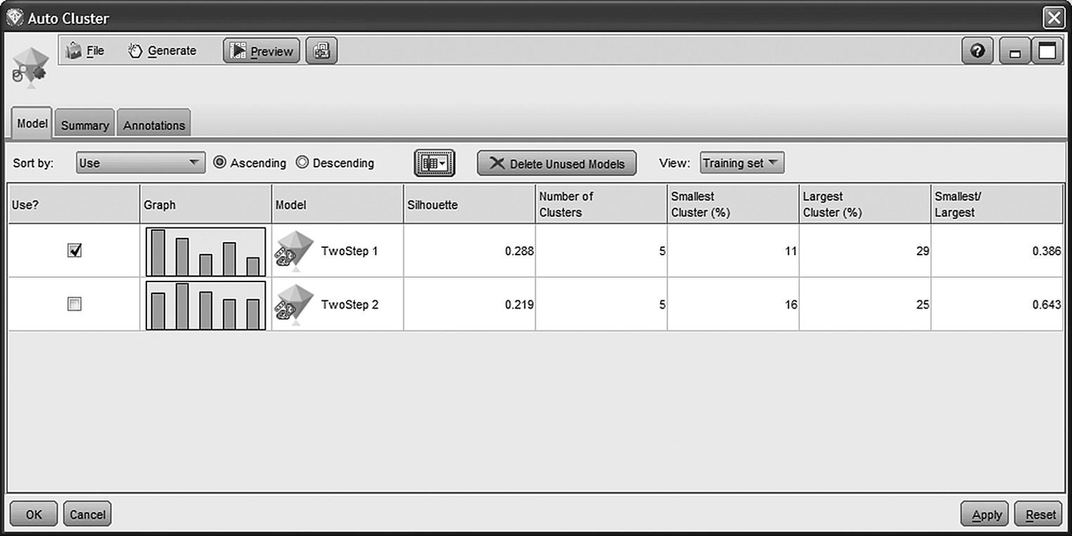
Figure 8.4 An initial comparison of the generated cluster models provided by the Auto Cluster model nugget
The cluster viewer presents the number of identified clusters as well as the Silhouette coefficient and the size of smallest and largest clusters for each model. In our case, the first TwoStep model was selected for deployment due to its higher Silhouette value and, more importantly, due to its transparency and interpretability.
The parameter settings of the selected cluster model are presented in Table 8.7.
Table 8.7 The parameter settings of the cluster model
| PCA model parameter settings | |
| Parameter | Setting |
| Model | TwoStep |
| Number of clusters | Automatically calculated |
| Exclude outliers option | On |
| Noise percentage | 10% |
As shown in Figure 8.5, the model yielded a five-cluster solution with a fair Silhouette measure of 0.29.

Figure 8.5 The Silhouette measure of the cluster model
The distribution of the revealed clusters is depicted in Figure 8.6.
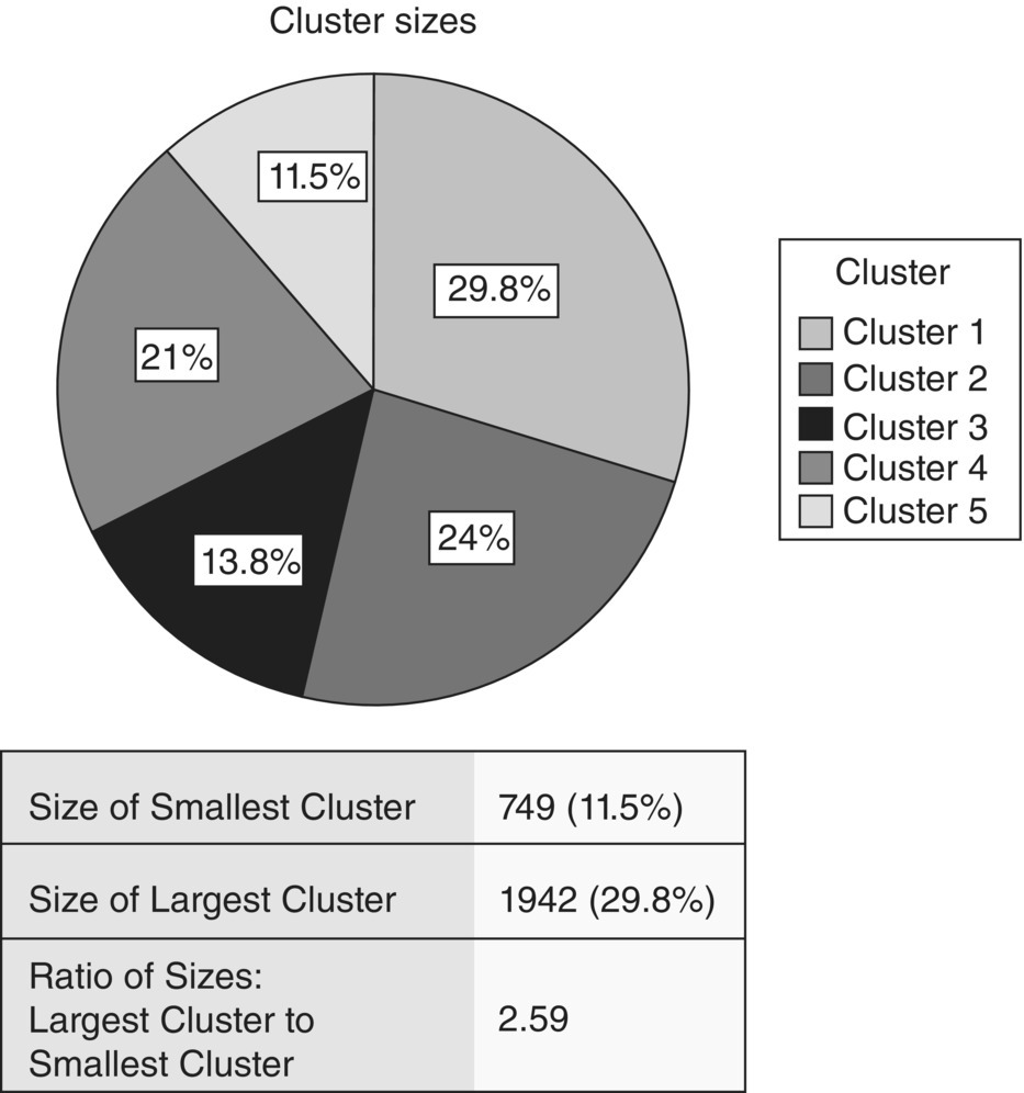
Figure 8.6 The distribution of the revealed clusters
As a reminder, we outline that these clusters were not known in advance, neither imposed by users, but uncovered after analyzing the actual behavioral patterns of the usage data. The largest cluster, Cluster 1, which as we’ll see corresponds to “typical” usage, contained about 30% of customers. The smallest one included about 11.5% of total users.
8.5.3 Profiling and understanding the clusters
Each revealed cluster corresponds to a distinct behavioral typology. This typology had to be understood, named, and communicated to all the people of the organization in a simple and concise way before being used for tailored interactions and targeted marketing activities. Therefore, the next phase of the project included the profiling of the clusters through simple reporting techniques. The “recognize and label” procedure started with the examination of the clusters in respect to the component scores, providing a valuable first insight on their structure, before moving to profiling in terms of the original usage fields. The table of centroids is shown in Figure 8.7.
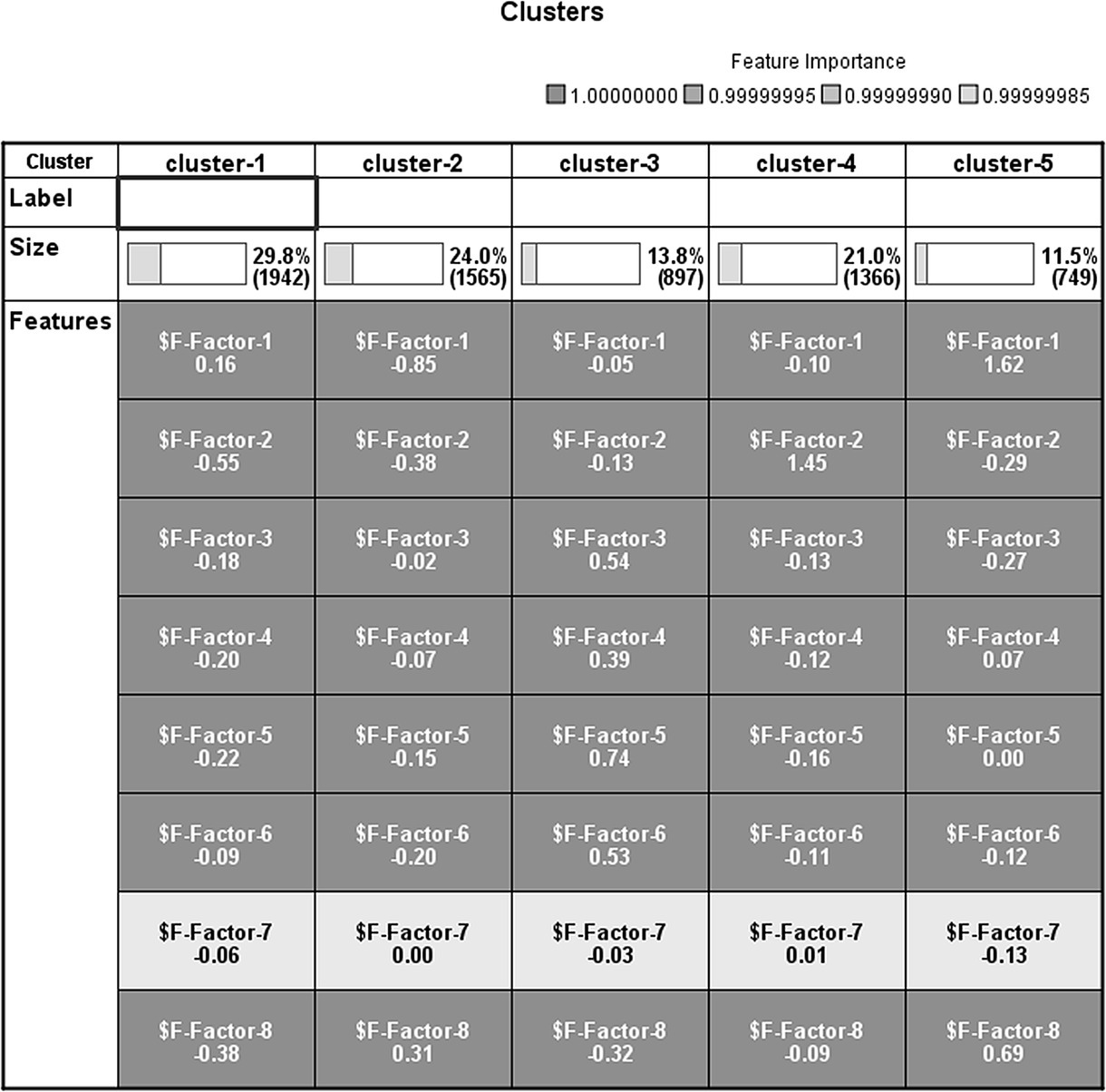
Figure 8.7 The table of centroids of the five clusters
Since the component scores are standardized, their overall means are 0 and the mean for each cluster denotes the signed deviation from the overall mean. By studying these deviations, we can see the relatively large mean values of Factors 1 and 8 among cases of Cluster 5. Since Factors 1 and 8 represent voice usage and average call duration, it seems that Cluster 5 was comprised of high voice users. This conclusion is further supported by studying the distribution of the factors for Cluster 5 with the series of boxplots presented in Figure 8.8.
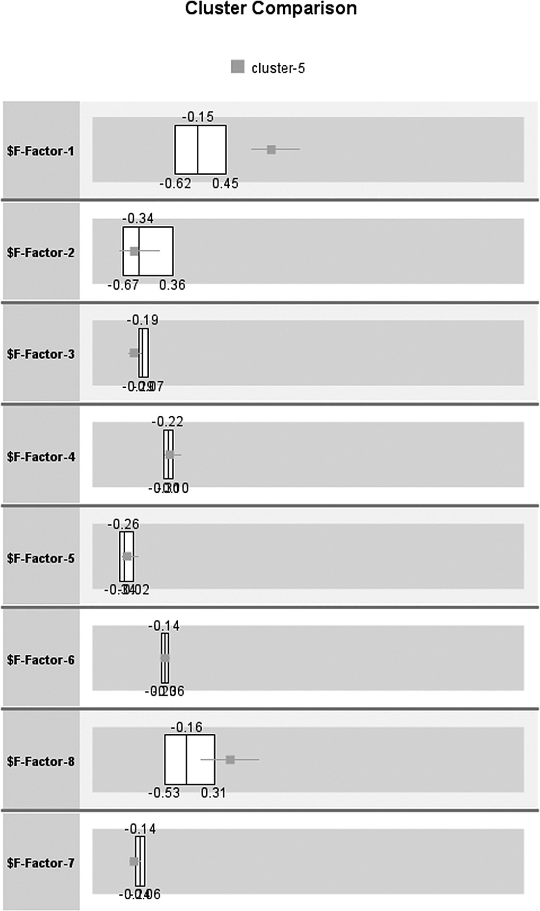
Figure 8.8 The distribution of factors for Cluster 5
The background boxplot summarizes the entire population, while the overlaid boxplot refers to the selected cluster. In respect to Factors 1 and 8, the boxplots for Cluster 5 are at the right side of those for the entire population, indicating high values and consequently high voice usage.
After studying the distributions of the factors, the profile of each cluster had started to take shape. In the final profiling stage, analysts returned to the primary inputs, seeking for more straightforward differentiations in terms of the original attributes. Table 8.8 summarizes the five clusters in terms of some important usage attributes. It presents the mean of each attribute over the members of each cluster. The last column denotes the overall mean.
Table 8.8 The means of some original attributes of importance for each cluster
| Clusters | ||||||
| Cluster 1 | Cluster 2 | Cluster 3 | Cluster 4 | Cluster 5 | Total | |
| VOICE_OUT_CALLS | 120 | 39 | 119 | 84 | 319 | 116 |
| PRC_VOICE_OUT_CALLS | 0.95 | 0.89 | 0.84 | 0.66 | 0.93 | 0.86 |
| VOICE_OUT_MINS | 92 | 37 | 108 | 77 | 357 | 108 |
| VOICE_IN_CALLS | 172 | 60 | 151 | 145 | 368 | 159 |
| VOICE_IN_MINS | 147 | 72 | 139 | 162 | 405 | 161 |
| OUT_COMMUNITY_VOICE | 31 | 12 | 30 | 22 | 67 | 29 |
| SMS_OUT_CALLS | 3 | 2 | 8 | 34 | 16 | 11 |
| PRC_SMS_OUT_CALLS | 0.02 | 0.04 | 0.05 | 0.25 | 0.05 | 0.08 |
| OUT_COMMUNITY_SMS | 1.57 | 1.06 | 3.44 | 8.89 | 5.36 | 3.67 |
| OUT_CALLS_ROAMING | 0.14 | 0.18 | 2.10 | 0.40 | 1.12 | 0.59 |
| OUT_MINS_ROAMING | 0.13 | 0.24 | 2.48 | 0.42 | 1.38 | 0.68 |
| OUT_CALLS_INTERNATIONAL | 0.29 | 0.21 | 2.81 | 0.53 | 1.06 | 0.76 |
| OUT_MINS_INTERNATIONAL | 0.36 | 0.32 | 4.42 | 0.74 | 1.86 | 1.16 |
| MMS_OUT_CALLS | 0.04 | 0.03 | 0.12 | 0.20 | 0.16 | 0.09 |
| INTERNET_CALLS | 0.07 | 0.03 | 0.93 | 0.15 | 0.17 | 0.21 |
| EVENTS_CALLS | 0.28 | 0.22 | 2.17 | 0.60 | 0.83 | 0.65 |
| OUT_COMMUNITY_TOTAL | 34 | 14 | 33 | 29 | 72 | 32 |
| DAYS_OUT | 25 | 16 | 23 | 23 | 28 | 23 |
| DAYS_IN | 26 | 18 | 24 | 24 | 28 | 24 |
| ACD_OUT | 0.75 | 0.93 | 0.89 | 0.86 | 1.17 | 0.88 |
| ACD_IN | 0.85 | 1.13 | 0.93 | 1.10 | 1.21 | 1.02 |
Large deviations from the marginal mean characterize the respective cluster and denote a behavior that differentiates the cluster from the typical behavior.
Although inferential statistics have not been applied to flag statistically significant differences from the overall population mean, we can see some large observed differences which seem to characterize the clusters. Based on the information summarized so far, the project team started to outline a first rough profile of each cluster:
- Cluster 1 contains average voice users.
- Cluster 2 seems to include users with basic usage. They also seem to be characterized by increased average call duration and very small communities.
- Cluster 3 includes roamers and users with increased communication with international destinations. They are also accustomed to Internet and event calls.
- Cluster 4 is mainly consisted of SMS users that seem to have an additional inclination to tech services like MMS, Internet, and event calls.
- Cluster 5 contains heavy voice users. They also have the largest outgoing communities. Perhaps, this segment included residential customers who use their phones for business purposes (self-professionals).
Although not presented here, the profiling of the clusters went on with demographical exploration and by assessing their revenue contribution. Additionally, the cohesion of the clusters was also examined mainly with boxplots and with dispersion measures, such as the standard deviations of the clustering fields for each cluster. Finally, a series of summarizing charts were built to graphically illustrate in an intuitive manner the cluster “structures.” The bars in the graphs represent the means of selected, important attributes, after standardization (in z-scores) over the members of the cluster. The vertical line at 0 denotes the overall mean. Hence, a bar facing to the right indicates a cluster mean higher than the overall mean, while a bar facing to the left indicates a lower mean. The bar charts are followed by a more detailed profiling of each cluster which wrap ups all their defining characteristics. The clusters were labeled according to these profiles (Figures 8.9, 8.10, 8.11, 8.12, and 8.13).
| Segment 1: typical voice users |
| Behavioral profile |
|
| Segment size |
| 29.8% |
| Segment 2: basic users |
| Behavioral profile |
|
| Segment size |
| 24% |
| Segment 3: international users |
| Behavioral profile |
|
| Segment size |
| 13.8% |
| Segment 4: young—SMS users |
| Behavioral profile |
|
| Segment size |
| 21% |
| Segment 5: professional users |
| Behavioral profile |
|
| Segment size |
| 11.5% |

Figure 8.9 Cluster 1 profiling chart
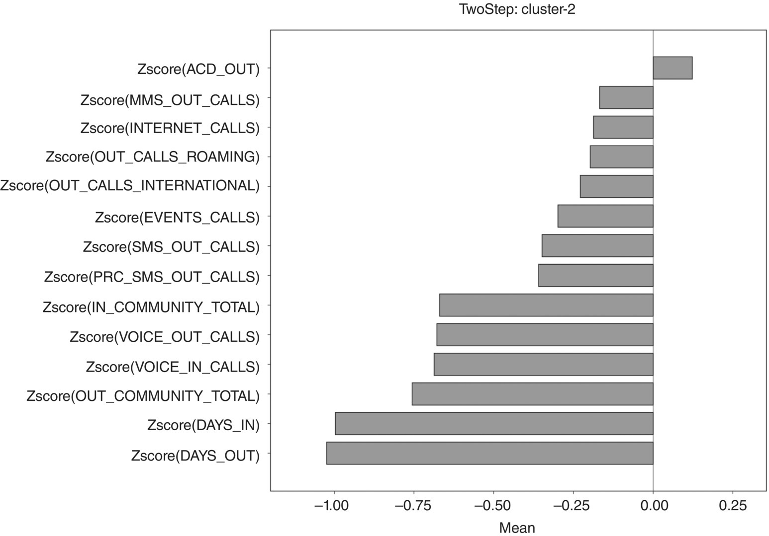
Figure 8.10 Cluster 2 profiling chart
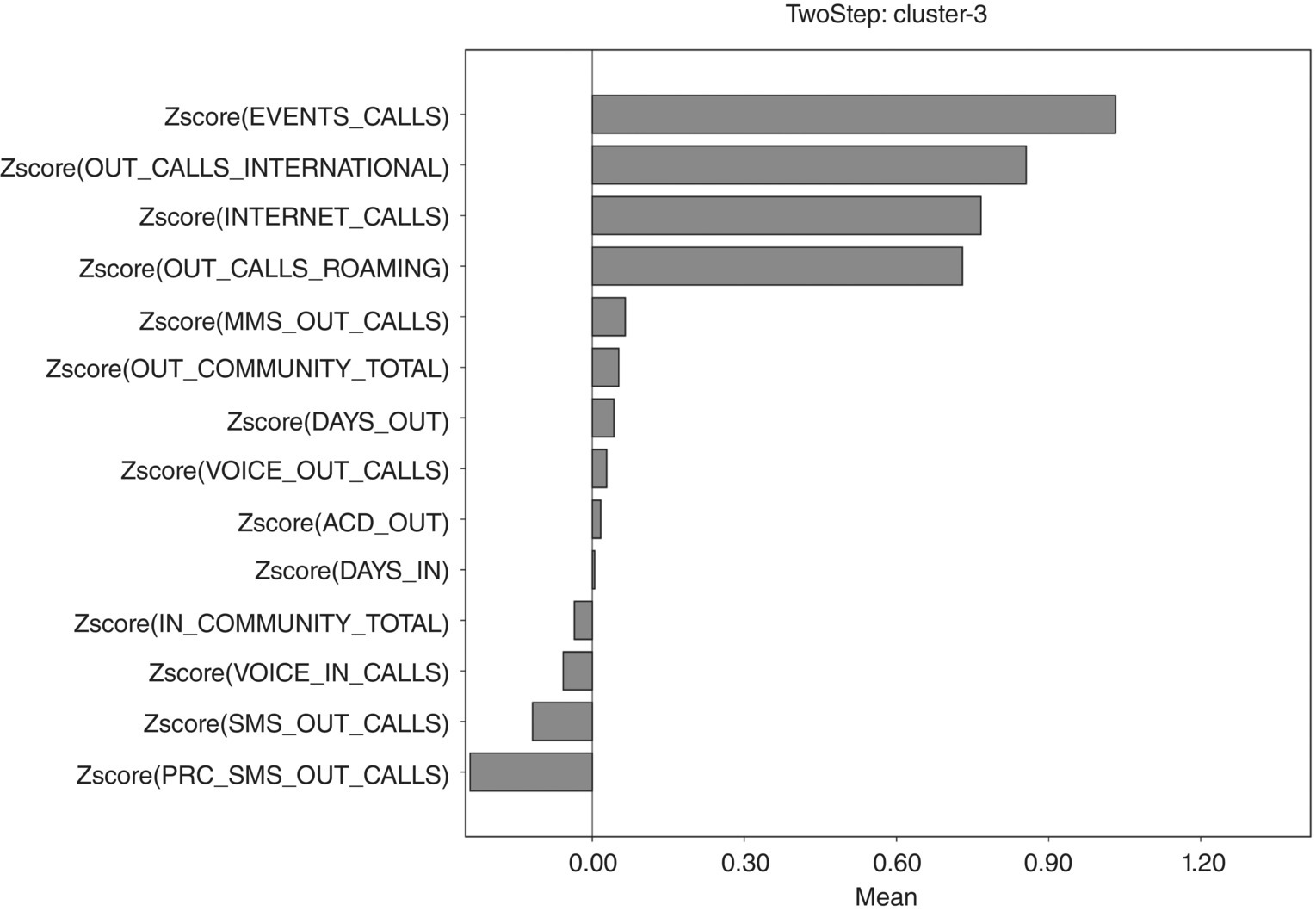
Figure 8.11 Cluster 3 profiling chart

Figure 8.12 Cluster 4 profiling chart
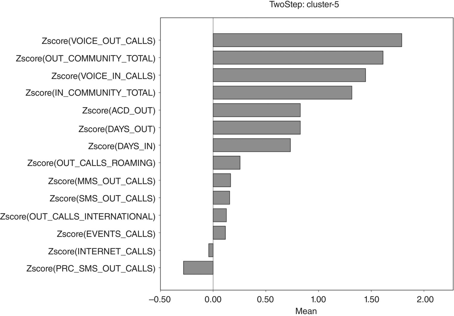
Figure 8.13 Cluster 5 profiling chart
8.5.4 Segmentation deployment
The final stage of the segmentation process involved the integration of the derived scheme in the company’s daily business procedures. From that moment, all customers were characterized by the segment to which they were assigned. The deployment procedure involved a regular (on a monthly basis) segment update. More importantly, the marketers of the operator decided to further study the revealed segments and enrich their profiles with attitudinal data collected through market research surveys. Finally, the organization used all the gained insight to design and deploy customized marketing strategies which improved the overall customer experience.
8.6 Segmentation using RapidMiner and K-means cluster
An alternative segmentation approach using the K-means algorithm and RapidMiner is presented in the following paragraphs.
8.6.1 Clustering with the K-means algorithm
A two-step approach was followed for clustering with RapidMiner. Initially, a PCA algorithm was applied for reducing the data dimensionality and for replacing the original inputs with fewer combined measures. Subsequently, the generated component scores were used as the clustering fields in a K-means algorithm which identified the distinct customer groupings. The RapidMiner process is presented in Figure 8.14.

Figure 8.14 The RapidMiner process for clustering
More specifically, a Retrieve operator was used to retrieve the modeling data from the RapidMiner repository. Then, through a Select Attributes operator, only the attributes designated as Inputs in Table 8.2 were retained for clustering. Since the PCA model in RapidMiner requires normalized inputs, the selected attributes were normalized with a Normalize operator. A z-normalization method was applied so eventually all attributes ended with a mean value of 0 and a standard deviation of 1. The z-scores were then fed into a PCA model operator with the parameter settings shown in Figure 8.15.

Figure 8.15 The PCA model settings
After trial and experimentation, a variance threshold of 85% was selected as the criterion for the extraction of components. This setting led to the extraction of 12 components which cumulatively accounted for about 85% of the total variance/information of the 31 original attributes, as shown in the rightmost column of the table in Figure 8.16. Initially, eight components were extracted which explained about 75% of the information of the original inputs. However, it turned out that the extraction of a larger number of components improved the K-means clustering, leading to a richer and more useful clustering solution. Therefore, the final choice was to proceed with the 12 components.

Figure 8.16 The variance explained by the components
The 12 components were then used as clustering inputs in a K-means model. The parameter settings are shown in Figure 8.17.
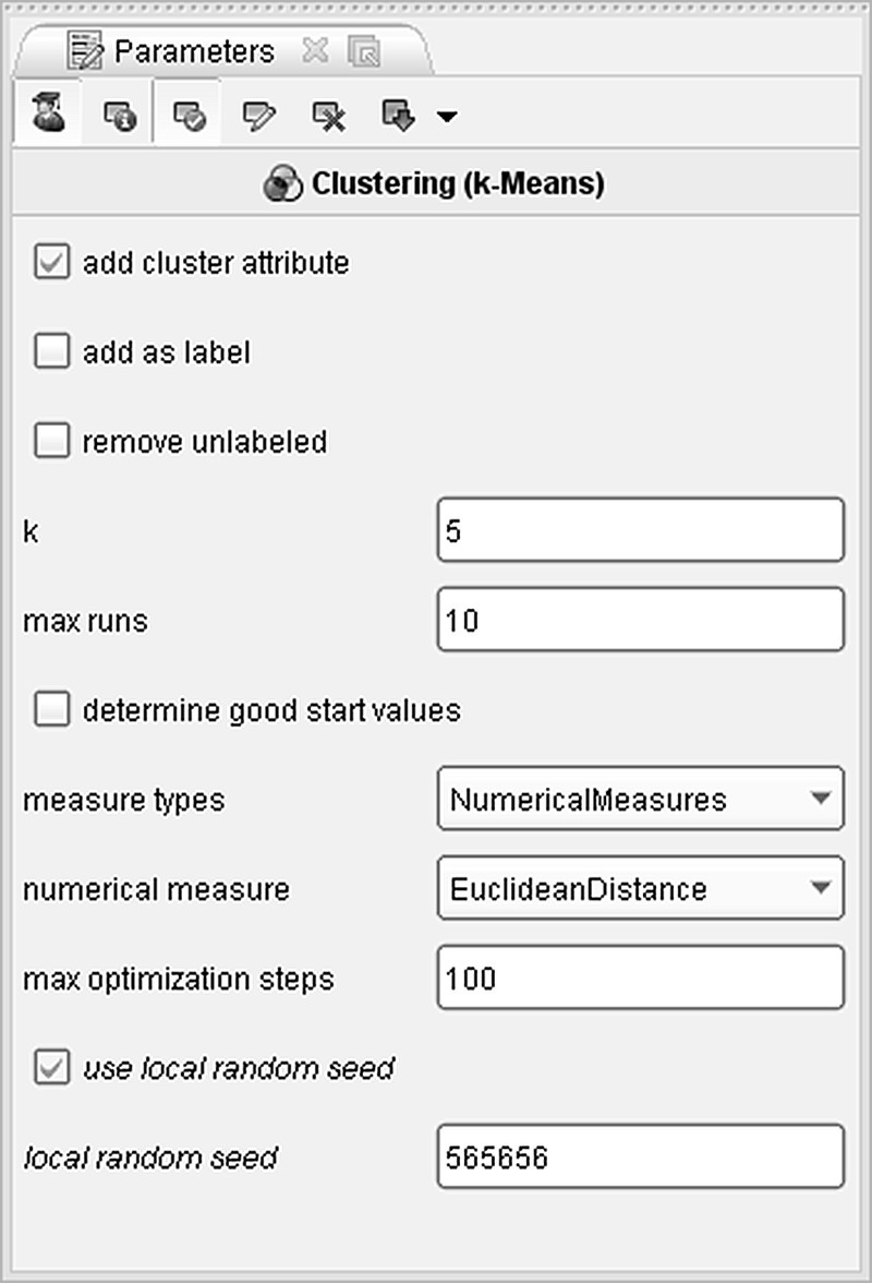
Figure 8.17 The K-means parameter settings
The Euclidean distance was selected for measuring the similarities of the records. The add-cluster attribute option generated the cluster membership field and assigned each instance to a cluster. After many trials and evaluations of many different clustering solutions, a 5-cluster solution was finally adopted for deployment. Hence, a “k” of 5 was specified, guiding the algorithm to form five clusters. The cluster distribution is presented in Figure 8.18. Clusters 3 and 4 are dominant since they comprise almost 80% of the total customer base.

Figure 8.18 The distribution of the K-means clusters
The generated K-means model was connected with a Cluster Distance Performance operator to evaluate the average distance between the instances and the centroid of their cluster. The respective results are shown in Figure 8.19.

Figure 8.19 Evaluating the cluster solution using within centroid distances
The segmentation procedure was concluded with the profiling of the revealed clusters and with the identification of their defining characteristics. The first step was to study the centroids table, available in the results tab of the cluster model. To facilitate additional profiling in terms of the original attributes, the cluster membership field was cross-examined with the original inputs. Figure 8.20 presents a profiling chart which depicts the averages of some important (normalized) attributes over the clusters. The vertical line at 0 corresponds to the marginal means of the normalized attributes. Hence, bars and dots to the right of this reference line designate cluster means above the marginal mean, while bars and dots to the left designate lower cluster means.
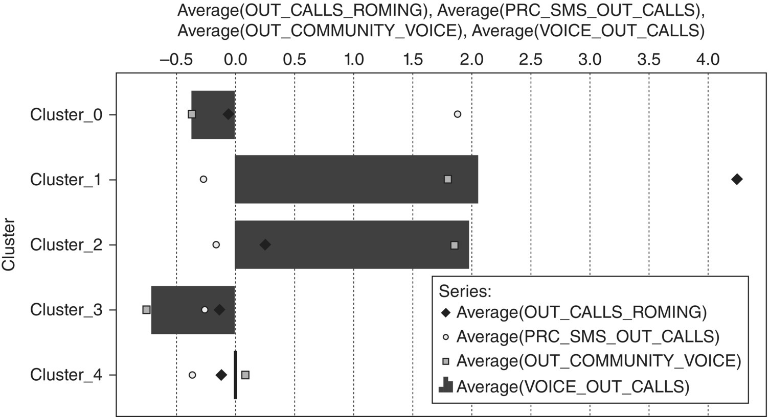
Figure 8.20 A profiling chart of the revealed clusters
A brief profile of the clusters is presented below. The clusters were named according to their identified characteristics:
- Cluster_0 SMS users: Highest SMS usage. Highest SMS to voice ratio. Increased usage of MMS, Events, and Internet
- Cluster_1 International users: Highest roaming and international usage. Also increased usage of voice and MMS
- Cluster_2 Professional users: High voice usage. Increased community, frequency (days), and duration of voice calls
- Cluster_3 Basic users: Lowest usage of all services and lowest community
- Cluster_4 Typical voice users: Average usage, almost exclusively voice
The revealed clusters seem indeed similar to the ones identified by the TwoStep algorithm. Tempted to compare the two solutions? After joining and cross-tabulating the cluster membership fields, it appears that the two models present an “agreement” of about 70%. Specifically, after excluding the TwoStep “outlier” cluster, the two models seem to assign approximately 70% of the instances in analogous groups. Where do they not agree? Their main difference is in the “international” segment which in the K-means solution is smaller, including only those roamers with increased general usage. The similarity of the clusters nevertheless is a good sign for the validity of the solutions.
8.7 Summary
In this chapter, we’ve followed the efforts of a mobile phone network operator to segment its customers according to their usage patterns. The business objective was to group customers in terms of their behavioral characteristics and to use this insight to deliver personalized customer handling. The first segmentation effort took into account the established core customer segments and initially focused on the residential postpaid customers which were further segregated into five behavioral segments, as summarized in Table 8.9. The procedure followed for the behavioral segmentation included the application of a PCA model for data reduction and a cluster model for revealing the distinct user groups.
Table 8.9 The mobile telephony segments
| Core segments | Residential customers | Postpaid—contractual |
| Behavioral segments | ||
| Typical voice users | ||
| Basic users | ||
| International users | ||
| SMS users | ||
| Professional users | ||
| Prepaid | ||
| Business customers | Large business—corporate | |
| Small medium enterprise—SME | ||
| Small office home office—SOHO |