
Chapter 31
VALUATION TECHNIQUES
That endless quest for fair value
Although you might not realise it, you already have the knowledge of all the tools that you will need to value a company. You discovered what discounting was about in Chapter 16 and learnt all about the right discount rate to use in Chapters 19 and 29. Finally, the comparable method was explained in Chapter 22. This chapter contains an in-depth look at the different valuation techniques and presents the problems (and solutions!) you will probably encounter when using them. Nevertheless, we want to stress that valuation is not a simple use of mathematical formulae, it requires the valuator to have good accounting and tax skills. You will also need to fully understand the business model of the firm to be valued in order to assess the reliability of the business plan supporting the valuation. Reading this chapter will only be a first step towards becoming a good valuator and, in addition, a great deal of practice and application will be needed.
Section 31.1 OVERVIEW OF THE DIFFERENT METHODS
Generally, we want to value a company in order to determine the value of its shares or of its equity capital.
Broadly speaking, there are two methods used to value equity: the direct method and the indirect method. In the direct method, obviously, we value equity directly. In the indirect method, we first value the firm as a whole (what we call “enterprise” or “firm” value), then subtract the value of net debt to get the equity value.

In addition, there are two approaches used in both the direct and indirect methods:
- The fundamental approach based on valuing either:
- a stream of dividends, which is the dividend discount model (DDM); or
- a stream of free cash flows, which is the discounted cash flow (DCF) method.
This approach attempts to determine the company's intrinsic value, in accordance with financial theory, by discounting cash flows to their present value using the required rate of return.
- The pragmatic approach of valuing the company by analogy with other assets or companies of the same type for which a value reference is available. This is the peer comparison method (often called the comparables method). Assuming markets are efficient, we should be able to infer the value of a company from the value of others.
| Indirect approach | Direct approach | |
|---|---|---|
| Intrinsic value method (discounted present value of financial flows) | Present value of free cash flows discounted at the weighted average cost of capital (k) – value of net debt | Present value of dividends at the cost of equity: kE |
| Peer comparison method (multiples of comparable companies) | EBITDA/EBIT multiple × EBITDA/EBIT – value of net debt | P/E × net income |
The sum-of-the-parts method consists of valuing the company as the sum of its assets less its net debt. However, this is more a combination of the techniques used in the direct and indirect methods rather than a method in its own right.
Lastly, we mention options theory, whose applications we have seen in Chapter 30 and will see in Chapter 34. In practice, very few will value equity capital by analogy to a call option on the assets of the company. The concept of real options, however, had its practical heyday at the height of the stock market folly of 1999 and 2000, to explain the market values of “new economy” stocks. Needless to say, this method has since fallen out of favour (but may come back to justify the valuation of some tech groups today).
If you remember the efficient market hypothesis, you are probably asking yourself why market value and discounted present value would ever differ. In this chapter we will take a look at the origin of the difference, and try to understand the reason for it and how long we think it will last. Ultimately, market values and discounted present values should converge.
Section 31.2 VALUATION BY DISCOUNTED CASH FLOW
The discounted cash flow method (DCF) consists of applying the investment decision techniques (see Chapter 16) to the firm value calculation. We will focus on the present value of the cash flows from the investment. This is the fundamental valuation method (or intrinsic method). Its aim is to value the company as a whole (i.e. to determine the value of the capital employed, what we call enterprise value). After deducting the value of net debt, the remainder is the value of the company's shareholders' equity.
As we have seen, the cash flows to be valued are the after-tax amounts produced by the firm. They should be discounted out to perpetuity at the company's weighted average cost of capital (see Chapter 29):
In practice, we project specific cash flows over a certain number of years. This period is called the explicit forecast period. The length of this period varies depending on the sector. It can be as short as two to three years for a high-tech company, five to seven years for a consumer goods company and as long as 20 to 30 years for a utility. For the years beyond the explicit forecast period, we establish a terminal value.
1/ SCHEDULE OF FREE CASH FLOWS
Free cash flows measure the cash-producing capacity of the company. Free cash flows are estimated as follows:
You buy a company for its future, not its past, no matter how successful it has been. Consequently, future cash flows are based on projections contained in the business plan of the company. As they will vary depending on growth assumptions, the most cautious approach is to set up several scenarios. But for starters, are you the buyer or the seller? The answer will influence your valuation. The objective of negotiation is to reconcile the buyer's and seller's points of view. We have found in our experience that discounted cash flow analysis is a very useful discussion tool: the seller gets accustomed to the idea of selling their company and the buyer gets a better understanding of the company for sale.
It is all right for a business plan to be optimistic – our bet is that you have never seen a pessimistic one – the important thing is how it stands up to scrutiny. It should be assumed that competition will ultimately eat into margins and that increases in profitability will not be sustained indefinitely without additional investment or additional hiring. Quantifying these crucial future developments means entering the inner sanctum of the company's strategy.
(a) Business plan horizon
The length of the explicit forecast period will depend on the company's “visibility” – i.e. the period of time over which is it reasonable to establish projections. This period is necessarily limited. In 10 years' time, for example, probably only a small portion of the company's profits will be derived from the production facilities it currently owns or from its current product portfolio. The company will have become a heterogeneous mix of the assets it has today and those it will have acquired over the next 10 years.
The forecast period should therefore correspond to the time during which the company will live off its current configuration. If it is too short, the terminal value will be too large and the valuation problem will only be shifted in time. Unfortunately, this happens all too often. If it is too long (more than 10 years), the explicit forecast is reduced to an uninteresting theoretical extrapolation.
Let's look at ArcelorMittal's financial projections and its stock trend chart. Below are a few projections that we made for teaching purposes, building on analysts' consensus.
| ($m) | 2020 | 2021e | 2022e | 2023e | 2024e | 2025e |
|---|---|---|---|---|---|---|
| Profit and loss statement | ||||||
| Turnover | 53,270 | 68,521 | 60,503 | 58,025 | 57,811 | 57,827 |
| EBITDA1 | 4,301 | 15,008 | 9,114 | 6,859 | 6,713 | 6,551 |
| − Depreciation and amortisation | 2,960 | 2,536 | 2,536 | 2,536 | 2,590 | 2,590 |
| = EBIT | 1,341 | 12,472 | 6,578 | 4,323 | 4,123 | 3,961 |
| Balance sheet | ||||||
| Fixed assets | 45,398 | 45,486 | 46,435 | 47,258 | 47,847 | 48,511 |
| + Working capital | 2,805 | 4,200 | 4,522 | 4,589 | 4,664 | 4,755 |
| = Capital employed | 48,203 | 49,686 | 50,957 | 51,847 | 52,511 | 53,266 |
| Operating margin after 20% tax | 1.9% | 13.7% | 8.2% | 5.6% | 5.3% | 5.1% |
| ROCE after 20% tax | 2.1% | 18.8% | 9.7% | 6.3% | 5.9% | 5.6% |
It should be noted that the ROCE at the end of the period (5.6%) is much lower than the cost of capital (10%) but on average over the period 2021–2025 (9.2%) it is quite close.
Projected after-tax free cash flows are as follows:
| ($m) | 2020 | 2021e | 2022e | 2023e | 2024e | 2025e |
|---|---|---|---|---|---|---|
| EBIT | 1,341 | 12,472 | 6,578 | 4,323 | 4,123 | 3,961 |
| − Corporate income tax at 25% | 335 | 3,118 | 1,645 | 1,081 | 1,031 | 990 |
| + Depreciation and amortisation | 2,960 | 2,536 | 2,536 | 2,789 | 2,800 | 2,912 |
| − Capital expenditure | 2,439 | 2,900 | 3,000 | 3,000 | 3,075 | 3,152 |
| − Changes in working capital | –1,841 | 1,395 | 322 | 67 | 75 | 91 |
| = Free cash flow | 3,368 | 7,595 | 4,148 | 2,964 | 2,742 | 2,640 |
Using a weighted average cost of capital of 10%, the end-2020 present value of the free cash flows generated during the explicit forecast period (2021–2025) is $16,071m.
Some practitioners discount cash flows over half years; the formula then becomes:

This assumes that cash flows are cashed in “on average” at half-year and that the valuation is performed at the beginning or end of the year.
(b) Terminal value
It is very difficult to estimate a terminal value because it represents the value at the date when existing business development projections will no longer have any meaning. Often analysts assume that the company enters a phase of maturity after the end of the explicit forecast period. In this case, the terminal value can be based either on the capital employed or on the free cash flow in the last year of the explicit forecast period.
The most commonly used terminal value formula is the Gordon–Shapiro formula. It consists of a normalised cash flow, or annuity, that grows at a rate (g) out to perpetuity:
Value of the company at the end of the explicit forecast period
However, the key challenge is in choosing the normalised free cash flow value and the perpetual growth rate. The normalised free cash flow must be consistent with the assumptions of the business plan. It depends on long-term growth, the company's investment strategy and the growth in the company's working capital. Lastly, normalised free cash flows may be different from the free cash flow in the last year of the explicit forecast period, because normalised cash flow is what the company will generate after the end of the explicit forecast period and will continue to generate to perpetuity.
Concerning the growth rate to perpetuity, do not get carried away:
- Apart from the normalised cash flow's growth rate to perpetuity, you must take a cold, hard look at your projected long-term growth in return on capital employed. How long can the economic profit it represents be sustained? How long will market growth last?
- Most importantly, the company's rate of growth to perpetuity cannot be significantly greater than the long-term growth rate of the economy as a whole. For example, if the anticipated long-term inflation rate is 2% and real GDP growth is expected to be 2%, then if you choose a growth rate g that is greater than 4%, you are implying that the company will not only outperform all of its rivals but also eventually take control of the economy of the entire country or indeed of the entire world (trees do not grow to the sky)!2
In the case of ArcelorMittal, the normalised cash flow must be calculated for the year 2026, because we are looking for the present value at the end of 2025 of the cash flows expected in 2026 and every subsequent year to perpetuity. Given the necessity to invest if growth is to be maintained, you could use the following assumptions to determine the normalised cash flow:
Using a rate of growth to perpetuity of 2%, we calculate a terminal value of $35,095m. Discounted over five years, this gives us $21,791m at the end of 2020. The enterprise value of ArcelorMittal is therefore $16,071m + $21,791m, or $37,863m. Note that the terminal value of $35,095m at end-2025 corresponds to a multiple of 8.9 times 2025 EBIT. This means that choosing a multiple of 8.9 is theoretically equivalent to applying a growth rate to perpetuity of 2% to the normalised cash flow and discounting it at the required rate of return of 10%.
Given a net debt of $14,000m, the equity value of ArcelorMittal as at end-2020 works out, with this method, at $23,863m.
Sometimes the terminal value is estimated based on a multiple of a measure of operating performance. This measure can be, among other things, turnover, EBITDA or EBIT. Generally, this “horizon multiple” is lower than an equivalent, currently observable, multiple. This is because it assumes that, all other things being equal, prospects for growth decrease with time, commanding a lower multiple. Nevertheless, since using this method to assess the terminal value implies mixing intrinsic values with comparative values, we strongly advise against it.
Computing the terminal value with a multiple prevents you from pondering over the level of ROCE that the company can maintain in the future.
Remember that if you compute a terminal value greater than book value, you are implying that the company will be able to maintain forever a return on capital employed in excess of its weighted average cost of capital. If you choose a lower value, you are implying that the company will enter a phase of decline after the explicit forecast period and that you think it will not be able to earn its cost of capital in the future. Lastly, if you assume that terminal value is equal to book value, you are implying that the company's economic profit3 falls immediately to zero. This is the method of choice in the mining industry, for example, where we estimate a liquidation value by summing the scrap value of the various assets – land, buildings, equipment – less the costs of restoring the site.
In the case of ArcelorMittal, the capital employed end-2025 is $53,266m, and discounted over five years at 10% results in $33,074m. With this method, the enterprise value as at end-2020 becomes 16,071 + 33,074 = $49,145m.
Generally speaking, no economic profit can be sustained forever. The company's expected return on capital employed must gradually converge towards its cost of capital. This is the case with Coca-Cola, Michelin or British Airways. Regardless of the calculation method, the terminal value must reflect this. To model this phenomenon, we recommend using a “cash flow fade” methodology. In this approach, you define a time period during which the company's return on capital employed diminishes, either because its margins shrink or because asset turnover declines. Ultimately, the ROCE falls down to the weighted average cost of capital. At the end of this time period, the enterprise value is equal to the book value of capital employed.

Readers will have to make choices: length of the cash flow fade period or speed of the convergence towards the cost of capital (form of the ROCE curve: convex, concave or a straight line as in our graph). They might also think that the company will be in a position to earn 1% or 2% more than its cost of capital due to the strength of its strategic position in its markets. Economic theory would not approve that!
This model can also be used for value-destroying companies. Sooner or later, there will be restructurings and bankruptcies triggering improvements in ROCE, but before applying the cash flow fade method the other way around, our readers would be well advised to ask themselves whether or not their company will be among the survivors!
2/ CHOOSING A DISCOUNT RATE
As we value cash flow to the firm, the discount rate is the weighted average cost of capital (WACC) or simply the cost of capital, which corresponds to the minimum rate of return required by the company's fund providers, i.e. shareholders and lenders to finance the company's capital employed. You may want to turn back to Chapter 29 for a more detailed look at this topic.
3/ THE VALUE OF NET DEBT
Once you obtain the enterprise value using the above methodology, you must remove the value of net debt taken at the date just before the start of the cashflows to be discounted (e.g. at 31 December 2020 for cashflows starting in 2021) to derive equity value. Net debt is composed of the value of all financial debt net of cash, i.e. of all bank borrowings, bonds, debentures and other financial instruments4 (short, medium or long-term), net of cash, cash equivalents and marketable securities.
Theoretically, the value of net debt is equal to the value of the future cash outflows (interest and principal payments) it represents, discounted at the market cost of similar borrowings. When all or part of the debt is listed or traded over the counter (listed bonds, syndicated loans), you can use the market value of the debt. You then subtract the market value of cash, cash equivalents and marketable securities.
The book value of net debt is often used as a first approximation of its present value. Nevertheless, in some cases, the value of debt can differ materially from its book value:
- when the firm has borrowed at fixed rates (directly after having swapped floating-rate debt) and rates have evolved since then;
- when the company's solvency situation has significantly changed (for better or worse) since it has contracted the debt and there has been no spread adjustment to recognise this change;
- when the interest rate has been artificially reduced thanks to the issue of debt with warrants or other products (note that this would nevertheless be restated in IFRS or US GAAP accounts).
Hence, we strongly advise retaining the market value of debt rather than its book value when the net debt is high and the difference between book and market value is material.
For example, as at 31 December 2020, the book value of Rallye's financial debt was €10,930m, its fair value was only €10,230m, a difference of €700m that represents twice the market capitalisation of Rallye as at mid-2021!
When the company's business is seasonal, year-end working capital may not reflect average requirements, and debt on the balance sheet at the end of the year may not represent real funding needs over the course of the year (see Chapter 11). Some companies also perform year-end “window-dressing” in order to show a very low level of net debt. In these cases, if you notice that interest expense does not correspond to debt balances,5 you should restate the amount of debt by using a monthly average of outstanding net debt, for example.
Some other items may add complexity in the assessment of the real level of debt. For example, if assets have been removed from the balance sheet thanks to factoring or securitisation, they need to be added back in. In other cases, sellers may try to “dress” the balance sheet to show a level of debt lower than reality.
4/ OTHER VALUATION ELEMENTS
(a) Provisions
Provisions must only be included if cash flows exclude them. If the business plan's EBIT does not reflect future charges for which provisions have been set aside – such as for restructuring, site closures, etc. – then the present value of the corresponding provisions on the balance sheet must be deducted from the value of the company after taxes (if the provision was not tax deductible).
Pension liabilities are a sticky problem (this is developed further in Chapter 7). How to handle them depends on how they were booked and, potentially, on the age pyramid of the company's workforce. You will have to examine the business plan to see whether it takes future pension payments into account and whether or not a large group of employees is to retire just after the end of the explicit forecast period.
With rare exceptions, deferred tax liabilities generally remain relatively stable. In practice, they are rarely paid out. Consequently, they are usually not considered debt equivalents.
(b) Unconsolidated or equity-accounted investments
If unconsolidated or equity-accounted financial investments are not reflected in the projected cash flows (via dividends received), you should add their value to the value of discounted cash flows. In this case, use the market value of these assets including, if relevant, tax on capital gains and losses.
For listed securities, use listed market value. Conversely, for minor, unlisted holdings, the book value is often used as a shortcut. However, if the company holds a significant stake in the associated company – this is sometimes the case for holdings booked using the equity method – you will have to value the affiliate separately. This may be a simple exercise, applying, for example, a sector-average P/E to the company's pro rata share of the net income of the affiliate. It can also be more detailed, by valuing the affiliate with a multi-criteria approach if the information is available.
(c) Tax-loss carryforwards
The value of any available tax loss carryforwards can be separately estimated by discounting the tax savings at the cost of capital until they are fully utilised. Alternatively, their use may be simulated in the calculation of free cash flow by using the standard tax rate only for the period following the exhaustion of the tax loss carryforwards.
(d) Minority interests
Future free cash flows calculated on the basis of consolidated financial information will belong partly to the shareholders of the parent company and partly to minority shareholders in subsidiary companies, if any.
This bias can be corrected by deducting minority interests from the enterprise value. If material, they should be valued separately and this can be done by performing a separate valuation of the subsidiaries in which some minority shareholders hold a stake. Naturally, this assumes you have access to detailed information about the subsidiaries.
You can also use a multiple approach. Simplifying to the extreme, you could apply the group's implied P/E multiple to the minority shareholders' portion of net profit to get a first-blush estimate of the value of minority interests. Alternatively, you could apply the group's price-to-book ratio to the minority interests appearing on the balance sheet.
In either case, we would not recommend using book value to value minority interests unless amounts are low.
(e) Dilution
You might be wondering what to do with instruments that give future access to company equity, such as convertible bonds, warrants and stock options. If these instruments have a market value, your best bet will be to subtract that value from the enterprise value of the company to derive the value of equity capital, just as you would for net debt. The number of shares to use in determining the value per share will then be the number of shares currently in circulation.
Alternatively, you could use the treasury stock method (see Section 22.5) to measure the impact of these instruments on the value of the shares. Its drawback lies in ignoring the value of out-of-the money dilutive instruments.
5/ PROS AND CONS OF THE CASH FLOW APPROACH
The advantage of the discounted cash flow approach is that it quantifies the often implicit assumptions and projections of buyers and sellers. It also makes it easier to keep your feet closer to the ground during periods of market euphoria, excessively high valuations and astronomical multiples. It forces the valuation to be based on the company's real economic performance.
You might be tempted to think this method works only to estimate the value of the majority shareholder's stake and not for estimating the discounted value of a flow of dividends. You might even be tempted to go a step further and apply a minority discount to the present value of future cash flows for valuing a minority holding.
This is wrong. Applying a minority discount to the discounted cash flow method implies that you think the majority shareholder is not managing the company fairly. A discount is justified only if there are “losses in transmission” between free cash flow and dividends. This can be the case if the company's strategy regarding dividends, borrowing and new investment is unsatisfactory.
Similarly, increasing the cash flow-based value can be justified only if the investor believes they can unlock synergies that will increase free cash flows.
To conclude, as satisfying as the DCF method is in theory, it presents three major drawbacks:
- It is very sensitive to assumptions and, consequently, the results it generates are very volatile. It is a rational method, but the difficulty in predicting the future brings significant uncertainty.
- It sometimes depends too much on the terminal value, in which case the problem is only shifted to a later period. Often the terminal value accounts for more than 50% of the value of the company, compromising the method's validity. However, it is sometimes the only applicable method, such as in the case of a loss-making company for which multiples are inapplicable.
- Lastly, it is not always easy to produce projections over a sufficiently long period of time. External analysts may often find they lack critical information.
6/ DISCOUNTING CASH FLOW AND DISCOUNTING DIVIDENDS
Before people grew accustomed to using the discounted free cash flow to firm method,6 the dividend discount model was very popular: the value of a share is equal to the present value of all the cash flows that its owner is entitled to receive, namely the dividends, discounted at the cost of equity (kE).
This method is not an easy one to carry out if there is a regular change in the financial structure, which prompts a regular change in the cost of equity. But it is widely used to value banks, whose financial structures do not change much over time as a result of the capital adequacy ratios they must respect.7
This method is still used in very specific cases – for example, for companies in mature sectors with very good visibility and high payout ratios, such as utilities, concessions and real-estate companies.
Using the same logic, one can compute the value of equity by discounting free cash flow to equity (and no longer to firm) at the cost of equity. Free cash flow to equity is money available for shareholders, i.e. free cash flow to the firm minus after-tax interest payments and plus changes in net debt. We find this method quite theoretical and complex as the cost of equity and therefore the discount rate changes every year with the financial structure.
Section 31.3 MULTIPLE APPROACH OR PEER-GROUP COMPARISONS
1/ PRESENTATION
The peer comparison or multiples approach (or comparables, “comps” method) is based on three fundamental principles:
- the company is to be valued in its entirety;
- the company is valued at a multiple of its profit-generating capacity. The most commonly used are the P/E ratio, EBITDA and EBIT multiples;
- markets are efficient and comparisons are therefore justified.
Much like the DCF model, the approach is global, because it is based not on the value of individual operating assets and liabilities per se, but on the overall returns they are expected to generate. The value of the company is derived by applying a certain multiplier to the company's profitability parameters. As we saw in Chapter 22, multiples depend on expected growth, risk and interest rates.
The approach is comparative. At a given point in time and in a given country, companies are bought and sold at a specific price level, represented, for example, by an EBIT multiple. These prices are based on internal parameters and by the overall stock market context. Prices paid for companies acquired in Europe in 2021, for example, when EBIT multiples were high (15 times on average) were not the same as for those acquired in 1980 when multiples hovered around four times EBIT.
Multiples can derive from a sample of comparable, listed companies or a sample of companies that have recently been sold. The latter sample has the virtue of representing actual transaction prices for the equity value of a company. These multiples are respectively called market multiples or trading multiples and transaction multiples. The first ones will be used to value shares of a firm that will not change control (for portfolio management or in the context of an IPO). The second ones are useful for assessing the value of equity in the context of change of control.
2/ BUILDING A SAMPLE OF COMPARABLE COMPANIES
For market multiples, a peer group comparison consists of setting up a sample of comparable listed companies that have not only similar sector and ideally geographic characteristics, but also similar operating characteristics, such as expected growth rates, size, etc. You should choose companies whose shares are liquid and are covered by a sufficient number of financial analysts.
3/ THE MENU OF MULTIPLES
There are two major groups of multiples: those based on the enterprise value (i.e. the value of capital employed), which is then used to obtain the value of equity, and those which are based directly on the value of equity.
Multiples based on the value of capital employed are multiples of operating balances before subtracting interest expense: EBIT and EBITDA multiples.
Multiples based on the value of equity are multiples of operating balances after interest expense, principally net income (P/E multiple), as well as multiples of cash flow and multiples of underlying income – i.e. before non-recurring items and the price book multiple (PBR).
(a) Multiples based on enterprise value
Whatever multiple you choose, you will have to value the capital employed for each listed company in the sample. This value is the sum of the company's market capitalisation (or transaction value of equity for transaction multiples) and the value of its net debt at the valuation date and other adjustments presented.
In any case you need to be clear: the value of a minority stake will be deducted from the enterprise value if no dividend has been included in the company parameter (EBIT or EBITDA, which is normally the case), but not if it is included (net income). If pension assets minus pension liabilities have been added to enterprise value, then the part of pension cost corresponding to the interest cost shall not be included in the EBIT or EBITDA,8 etc.
You will then calculate the multiple for the comparable companies over three fiscal years: the current year, last year and next year. Note that we use the same value of capital employed in all three cases, as current market values should reflect anticipated changes in future operating results.9
Once the multiples of the comparable companies have been calculated and applied to the corresponding aggregates of the company to be valued, the value of the net debt and similar items presented on page 563 should be deducted from the value of the enterprise value arrived at in this way. The only case where the net debt included in these two valuation methods could be different is the subject of question 19 at the end of this chapter.
EBIT multiple
The EBIT multiple is the ratio of the enterprise value to EBIT (operating income). It takes into account the genuine profit-generating capacity of the sample companies.
You may have to perform some restatements in order to derive this operating income.
Consider the following sample of listed companies comparable to ArcelorMittal:
| €m | ThyssenKrupp | Voestalpine | Salzgitter | Nippon Steel | US Steel |
|---|---|---|---|---|---|
| Market capitalisation (value of equity) | 6,000 | 6,580 | 1,600 | 14,552 | 5,715 |
| + Value of debt | –3,782 | 3,281 | 879 | 17,135 | 2,565 |
| = Value of capital employed (A) | 2,218 | 9,087 | 2,479 | 31,687 | 8,280 |
| 2021e Operating income (EBIT) (B) | 424 | 782 | 366 | 4,104 | 1,848 |
| 2021e EBIT multiple (A/B) | 5.2 x | 11.6 x | 6.8 x | 7.7 x | 4.5 x |
The 2021 average pre-tax operating income (EBIT) multiple is 7.2 times. Applied to ArcelorMittal's 2021e operating income of $5,564m, comparable multiples would value ArcelorMittal's enterprise value at $40,584m and equity at $26,584m, taking into account $14,000m of debts.
EBITDA multiple
The EBITDA multiple follows the same logic as the EBIT multiple. It has the merit of eliminating the sometimes significant differences in depreciation methods and periods. It is very frequently used by stock market analysts for companies in capital-intensive industries which therefore record significant depreciation and amortisation charges.
Be careful when using the EBITDA multiple, however, especially when the sample and the company to be valued have widely disparate levels of margins. In these cases, the EBITDA multiple tends to overvalue companies with low margins and undervalue companies with high margins, independently of depreciation policy. Let's take the following example:
| Group A | Group B | |
|---|---|---|
| Sales | 100 | 100 |
| EBITDA | 20 | 11 |
| Depreciation | 10 | 10 |
| EBIT | 10 | 1 |
| Enterprise value | 140 | ? |
Group A is valued at seven times its EBITDA. If we use this same multiple to value Group B, we derive an enterprise value for Group B of 77 (11 × 7). But if the cost structure of Group B remains the same in the future, its EBIT will always be close to 0; if that is the case, an investor would have difficulties paying a lot for such a company. The value of such a firm should be close to nil. This is the result we find if we prefer the EBIT multiple to the EBITDA multiple.
Other multiples
Operating multiples can also be calculated on the basis of other measures, such as turnover. Some industries have even more specific multiples, such as multiples of the number of subscribers, number of visitors or page views for Internet companies, tons of cement produced, etc. These multiples are particularly interesting when the return on capital employed of the companies in the sample is standard. Otherwise, results will be too widely dispersed. They are only meaningful for small businesses such as shops, where there are a lot of transactions and where, in many countries, turnover gives a better view of the profitability than the official profit figure.
These multiples are generally used to value companies that are not yet profitable: they were widely used during the Internet bubble, for instance. They tend to ascribe far too much value to the company to be valued, and we recommend that you avoid them.
(b) Multiples based on equity value
You may also decide to choose multiples based on operating balances after interest expense. These multiples include the P/E ratio, the cash flow multiple and the price-to-book ratio. All these multiples use market capitalisation at the valuation date (or price paid for the equity for transaction multiples) as their numerator. The denominators are net profit, cash flow and book equity, respectively. The net profit used by analysts is the company's bottom line, i.e. the net profit attributable to the group (after deduction of minority interests) restated to exclude non-recurring items and the depreciation of goodwill, so as to put the emphasis on recurrent profit-generating capacity.
Using the same sample of comparable comparisons for ArcelorMittal presented before, we notice that the P/E ratio in 2021 for companies comparable to ArcelorMittal is 7.6:
| €m | ThyssenKrupp | Voestalpine | Salzgitter | Nippon Steel | US Steel |
|---|---|---|---|---|---|
| Market capitalisation (A) | 6,000 | 6,580 | 1,600 | 14,552 | 5,715 |
| 2017e Net income (B) | –278 | 528 | 241 | 1,820 | 1,652 |
| P/E ratio (A)/(B) | n.m. | 12.5 x | 6.6 x | 8.0 x | 3.5 x |
Applied to ArcelorMittal's 2021e net income prediction of €3,790m, comparable multiples would value ArcelorMittal's equity at €28,952m.
These multiples indirectly value the company's financial structure, thus creating distortions depending on whether or not the companies in the sample are indebted.
Consider the following two similarly sized companies, Ann and Valeria, operating in the same sector and enjoying the same outlook for the future, with the following characteristics:
| Company | Ann | Valeria | |
|---|---|---|---|
| Operating income (EBIT) | 129 | 177 | |
| − | Interest expense | 9 | 120 |
| − | Corporate income tax (30%) | 36 | 17 |
| = | Net profit | 84 | 40 |
| Value of equity | 2,100 | ? | |
| Value of debt (at 3% and 10% p.a. respectively) | 300 | 1,200 |
Ann's P/E ratio is 25 (2,100 / 84). As the two companies are comparable, we might be tempted to apply Ann's P/E ratio to Valeria's bottom line to obtain Valeria's value of equity – i.e. 25 × 40 = 1,000.
Although it looks logical, this reasoning is flawed. Applying a P/E ratio of 25 to Valeria's net income is tantamount to applying a P/E of 25 to Valeria's NOPAT (177 × (1 – 30%) = 124) less a P/E of 25 applied to its after-tax interest expense (120 × (1 – 30%) = 84). After all, net income is equal to net operating profit after tax less interest expense after tax.
The first term (25 × NOPAT) should represent the enterprise value of Valeria, i.e. 25 × 124 = 3,100.
The second term (25 × after-tax interest expense) should thus represent the value of debt to be subtracted from enterprise value to give the value of equity capital that we are seeking. However, 25 × interest expense after tax is 2,100, whereas the value of the debt is only 1,200.
In this case, this type of reasoning would result in overstating the value of the debt (at 2,100 instead of 1,200) and then understating the value of the company's equity.
The proper reasoning is as follows: we first use the multiple of Ann's EBIT to get Valeria's enterprise value. If Ann's equity value is 2,100 and its debt is worth 300, then its enterprise value is 2,100 + 300, or 2,400. As Ann's EBIT is 129, the multiple of Ann's EBIT is 2,400 / 129 = 18.6. Valeria's enterprise value is therefore equal to 18.6 times its EBIT, or 18.6 × 177 = 3,293. We now subtract the value of the debt (1,200) to obtain the value of equity capital, or 2,093. This is not the same as 1,000!
These distortions are the reason why financial analysts mostly use multiples of operating income (EBIT) or of operating income before depreciation and amortisation (EBITDA). This approach removes the bias introduced by different financial structures.
4/ TRANSACTION MULTIPLES
The approach is slightly different, but the method of calculation is the same. The sample is composed of information available on recent transactions in the same sector, such as the sale of a controlling block of shares, a merger, etc.
If we use the price paid by the acquirer, our multiple will contain the control premium the acquirer paid to obtain control of the target company. As such, the price includes the value of anticipated synergies. Using the listed share prices leads to a so-called minority value, which we now know is nothing other than the standalone value. In contrast, transaction multiples reflect majority value – i.e. the value including any control premium for synergies. For listed companies it has been empirically observed that control premiums are around 25% to 30% of pre-bid market prices (i.e. prices prior to the announcement of the tender offer).
You will find that it is often difficult to apply this method, because good information on truly comparable transactions is often lacking or incomplete (price paid not made public, unknown aggregates when the company is private, etc.).
As an example, the EBITDA multiples used in Europe for medium-sized company transfers are given in Section 31.6.
5/ MEDIANS, MEANS AND REGRESSIONS
People often ask if they should value a company by multiplying its profit-generating capacity by the mean or the median of the multiples of the sample of comparable companies. Our advice is to be wary of both means and medians, as they can mask wide disparities within the sample, and sometimes may contain extreme situations that should be excluded altogether. Try to understand why the differences exist in the first place rather than burying them in a mean or median value that has little real significance. For example, look at the multiples of the companies in the sample as a function of their expected growth. Sometimes this can be a very useful tool in positioning the company to be valued in the context of the sample.
Some analysts perform linear regressions to find a relationship between, for example, the EBIT multiple and expected growth in EBIT, the multiple of turnover and the operating margin, and the price-to-book ratio and the return on equity (to value banks).
This method allows us to position the company to be valued within the sample. The issue remaining, then, is to find the most relevant criterion. R2 indicates the significance of the regression line, and will be our guide in determining which criteria are the most relevant in the industry in question. Sometimes it allows you to choose a multiple outside the range of comparables' multiples, simply because the company you are valuing has higher or lower expected growth than others you are comparing it with.
Section 31.4 THE SUM-OF-THE-PARTS METHOD (SOTP) OR NET ASSET VALUE (NAV)
The sum-of-the-parts method is simple. It consists in systematically studying the value of each asset and each liability on the company's balance sheet. For a variety of reasons – accounting, tax, historical – book values are often far from reality. They must therefore be restated and revalued before they can be assumed to reflect a true net asset value. The sum-of-the-parts method is an additive method. Revalued assets are summed, and the total of revalued liabilities is subtracted.
For diversified groups, the SOTP or NAV method implies valuing subsidiaries or activities pro rata the ownership level using either the DCF or the multiples of comparable companies method. Then, the debt of the mother company10 is deducted as well as the present value of central costs. For example, UBS issued the following valuation in mid-2019 for Vivendi, a media group:
| Value | Valuation method | |
|---|---|---|
| Universal Music Group (80%) | 30,884 | Recent transaction |
| Canal+ (89%) | 4,896 | 2022 EBITDA multiple |
| Havas | 2,209 | 2022 EBITDA multiple |
| Editis | 663 | 2022 EBITDA multiple |
| Gameloft | 813 | Sales multiple |
| Vivendi Village | 47 | Sales multiple |
| Holding company and others | –1,423 | Cost multiple |
| Total enterprise value | 38,089 | |
| + Listed minority holdings | 3,513 | |
| incl. Telecom Italia (23.87%) | 1,594 | Stock market price |
| incl. Mediaset (28.8%) | 804 | Stock market price |
| inc. Lagardere (28.3%) | 835 | Stock market price |
| inc. Other (Prisa, Multichoice) | 279 | Stock market price |
| Non Listed minority holdings | 1,237 | |
| – Adjusted net debt (2021 Y/E) | –3,402 | |
| Equity value | 39,437 |
To apply this method properly, therefore, we must value each asset and each liability. Estimates must be consistent, even though the methods applied might be different.
Several basic types of value are used in the sum-of-the-parts method:
- market value: this is the value we could obtain by selling the asset. This value might seem indisputable from a theoretical point of view, but it virtually assumes that the buyer's goal is liquidation. This is rarely the case. Acquisitions are usually motivated by the promise of industrial or commercial synergies;
- value in use: this is the value of an asset that is used in the company's operations. It is a kind of market value at replacement cost;
- liquidation value: this is the value of an asset during a fire sale to get cash as soon as possible to avoid bankruptcy. It is market value minus a discount.
The sum-of-the-parts method is the easiest to use and the values it generates are the least questionable when the assets have a value on a market that is independent of the company's operations, such as the property market, the market for aeroplanes, etc. It is hard to put a figure on a new factory in a new industrial estate. However, the value of the inventories and vineyards of a wine company is easy to determine and relatively undisputed, since a secondary market exists for these assets.
1/ TANGIBLE ASSETS
Tangible assets can be evaluated on the basis of replacement value, liquidation value, going-concern value or yet other values.
We do not intend to go into great detail here. Our main point is that in the sum-of-the-parts method it is important to determine an overall value for productive and commercial assets. Rather than trying to decompose assets into small units, you should reason on a general basis and consider sufficiently large groups of assets that have a standalone value (i.e. for which a market exists or that can operate on a standalone basis).
For example, it makes no sense to value the land on which a warehouse has been built. It makes more sense to value the combination of the land and the buildings on it. An appraiser will value the combination based on its potential productive capacity, not on the basis of its individual components. Of course, this is not the case if the objective is to reuse the land for something else, in which case you will want to deduct the cost of knocking down the warehouse.
2/ INVENTORIES
For industrial companies, valuing inventories usually does not pose a major problem, unless they contain products that are obsolete or in poor condition. In this case, we have to apply a discount to their book value, based on a routine inventory of the products.
In some situations, you will have to revalue the inventories of companies with long production cycles; the revaluation can lead to gains on inventories. This is often the case with champagne and cognac or even losses on completion not yet booked. The revaluations need to include their corporate income tax impact. In revaluing inventories, you must be aware that we are already buying the profits of the next few years.
3/ INTANGIBLE ASSETS
It might seem paradoxical to value intangible assets, since their liquidation value has, for a long time, been considered to be low. It is now widely acknowledged, however, that the value of a company is partly determined by the real value of its intangible assets, be they brand names, a geographical location or other advantages.
Some noteworthy examples:
- Brands: particularly hard to value but the importance of brands in valuation is growing.
In general, there are three methods for valuing brands:
- Method 1 The first method asks how much would have to be spent in advertising expense, after tax, to rebuild the brand. This method leads to undervaluation of new and successful brands (Netflix) and overvaluation of older and failing brands (the Amazon Fire phone).
- Method 2 The second method calculates the present value of all royalty payments that will or could be received from the use of the brand by a third party. It is very sensitive to the chosen royalty rate.
- Method 3 The third method consists in analysing the brand's fundamental utility. After all, the brand's raison d'être is to enable the company to sell more and at higher prices than would otherwise be possible without the brand name (costs of enhanced quality and services, of communication). Discounting this “excess profit” over a certain period of time should, after subtracting the related higher costs, yield an estimate of the value of the brand. Users of this method discount the incremental future operating income expected from the use of the brand and subtract the additional operating expense, working capital and investments, thereby isolating the value of the brand. We will not hide the fact that this approach, while intellectually appealing, is very difficult to apply in practice, because often there is no generic “control” product to use as a benchmark.
- Patents and technical know-how: they are valued as brands, but with the same difficulties.
- Lease rights: the present value of the difference between market rental rates and the rent paid by the company.
4/ TAX IMPLICATIONS
The acquirer's objectives will influence the way taxes are included (or not) in the sum-of-the-parts approach.
- If the objective is to liquidate or break up the target company into component parts, then the acquirer will buy the assets directly, giving rise to capital gains or losses. The taxes (or tax credits) theoretically generated will then decrease (increase) the ultimate value of the asset.
- If the objective is to acquire some assets (and liabilities), and to run them as a going concern, then the assets will be revalued through the transaction. Increased depreciation will then lower income tax compared to liquidation or the breakup case above.11
- If the objective is to acquire a company and maintain it as a going concern (i.e. not discontinue its activities) and as a separate entity, then the acquiring company buys the shares of the target company rather than the underlying assets. It cannot revalue the assets on its books and will depreciate them from a lower base than if it had acquired the assets directly. As a result, depreciation expense will be lower and taxes higher.
5/ USEFULNESS OF SUM-OF-THE-PARTS VALUES
Sum-of-the-parts values can be deceptive, as many people think they imply safe or reliable values. In fact, when we say that a company has a high net asset value, it means that from a free cash flow point of view, the company's terminal value is high compared with the value of intermediate cash flows. Consequently, the more “net asset value” a company has and the fewer cash flows it has, the more speculative and volatile its value is. Granted, its industrial risk may be lower, but most of the value derives from speculation about resale prices.
For this reason, the sum-of-the-parts method is useful for valuing small companies with no particular strategic value, or companies whose assets can be sold readily on a secondary market (aeroplanes, cinemas, etc.).
Section 31.5 COMPARISON OF VALUATION METHODS
1/ RECONCILING THE DIFFERENT METHODS OF VALUATION
If markets are efficient, then all of the valuation methods discussed so far should lead to the same valuation. In reality, however, there are often differences among the sum-of-the-parts value, the DCF-based value and the peer-comparison value. You must analyse the source of these differences and resist the temptation to average them!
(a) Analysing the difference between sum-of-the-parts value and discounted cash flow value
If the sum-of-the-parts value is higher than the DCF value or the value derived from a comparison of multiples (both return based values), then the company is being valued more for its past, its revalued equity capital, than for its outlook for future profitability. In this case, the company should not invest but divest, liquidating its assets to boost profitability and improve the allocation of its resources. This is often the punishment for overly complacent management.
This strategy occurs at regular intervals (in the 1980s, in 2007–2008). Companies were bought up on the open market, and then sold off piecemeal. The buyer realises a gain because the parts are worth more than the company as a whole. Alternatively, often under pressure from activist investors (Chapter 41), the company can of its own volition embark on this refocusing process (General Electric, ThyssenKrupp, Seimens).
If the sum-of-the-parts value is lower than the DCF value or the value derived from multiples, which is the usual case in an economy where companies have a lot of intangibles, then the company is very profitable and invests in projects with expected profitability greater than their cost of capital. The company has real expertise, strong strategic positioning and enjoys high barriers to entry. But the chances are that it will not escape competitive pressure forever.
Goodwill value has long been used to correct the restated net asset value to take into account the anticipated return on capital employed of the firm compared to its cost of capital and hence to value its “intangible capital”.
The starting point of all these mixed methods was to determine the capital employed, restated for potential capital gains or losses. Then a normative operating profit was computed by applying the cost of capital to the capital employed. The difference between the actual operating profit and the normative operating profit was called super-profit (leading to goodwill if positive and badwill if negative). The super-profit is to be discounted over a certain period to derive the value of goodwill. This is conceptually close to the EVA.
(b) Comparison values versus DCF values
If the value obtained via peer comparison is greater than the DCF-based value (and if all the calculations are correct!), then the company's managers should be thinking about floating the company on the stock exchange, because financial investors have a more positive view of the company's risk profile and profitability outlook than its management or current shareholders. Conversely, if the value obtained by comparison is lower than the DCF value and if the business plan is reliable, it would be wiser to wait until more of the long-term growth potential in the company's business plan feeds through to its financial statements before launching an IPO; and perhaps do a public-to-private (see Section 47.2, 2/) if the company is already listed.
If transaction multiples generate a significantly higher value than market multiples or the DCF model, then it would be better to organise a trade sale by soliciting bids from several industry participants. In short, look before you leap!
(c) Is there one valuation method for selling a company and another for buying it?
There is no technical reason why a seller should not use one valuation method and the buyer another:
- A seller usually favours the DCF method as it is based upon a business plan which is rarely built on pessimistic assumptions! Most business plans are established by the management under instruction from selling shareholders. But in the back of their mind, a seller will not forget results obtained with a peer-comparison method, as they will be very reluctant to sell at a lower multiple than the one obtained by a competitor a few months ago or the one they could get through an IPO.
- A buyer will use the peer-comparison method to justify a lower price than that resulting from the DCF. They will claim that other buyers have paid 100 and there is no reason why they should pay 120 or 130. Nevertheless, at the back of their mind the buyer is thinking about their own business plan, including synergies and new developments. They will soon be able to compute their own DCF to check whether the price they will pay is expected to create value for their own shareholders.
2/ THE LIFECYCLE THEORY OF COMPANY VALUE
Companies that have achieved a certain level of success will see their sum-of-the-parts and cash flow values differ throughout their lifecycle. Lifecycle is an important factor in determining the value of companies, as it was in determining the optimal capital structure and financing policies.
When the company is founded, its net asset value and cash flow value are identical; the company has not yet made any investments. After the first year or two of operations, net asset value may dip because of start-up losses. Meanwhile, cash flow value is greater because it anticipates hopefully positive future profitability.
During the growth phase, net asset value will rise as all or part of the company's profits are reinvested and the company builds a customer base (the value of which does not appear in the accounts, however). Cash flow value also continues to rise and remains above the net asset value. The company's expertise has not yet become a tangible asset. It is still associated with the people who developed it.
At maturity, cash flow value will start growing more slowly or stop growing altogether, reflecting a normal profit trend. Nonetheless, the net asset value continues to grow, but more slowly because the company increases its payout ratio. Broadly speaking, net asset value and cash flow value are very close.
If the company then enters a phase of decline, its profits decline and the cash flow value slips below net asset value. The latter continues to grow but only very slowly, until the company starts posting losses. The net asset value falls. As for cash flow value, it drops very low. The net asset value then becomes particularly speculative.

At any given point in time, it is very important to understand the reasons for the difference between the net asset value and the cash flow value, because this understanding gives important clues as to the situation and future prospects of the company.
You might now be thinking that our kaleidoscope of methods leads to as many values as there are images of the company:
- sum-of-the-parts, or net asset value;
- peer-comparison value;
- intrinsic value (i.e. DCF), etc.
We advise against calculating a wide variety of valuations, unless it is to show that you can prove anything when it comes to valuation. But you must not throw up your hands in despair either. Instead, try to understand each type of value, which corporate circumstances it applies to and what its implicit assumptions are. It is more important to determine ranges than to come up with precise values. Precision is the domain of negotiation, the goal of which is to arrive at an agreed price.
Lastly, remember that valuing a company means:
- taking a speculative stance not only on the future of the company, but also on its market conditions. The cash flow and comparison methods demonstrate this;
- implicitly extrapolating past results or expected near-term results far into the future, opening the door to exaggeration;
- sometimes forgetting that net asset value is not a good reference if the profitability of the company differs significantly from its investors' required return.
Shareholders' decisions to sell all or part of a company are based on the price they believe they can obtain compared to their set of calculated valuations.
Section 31.6 PREMIUMS AND DISCOUNTS
A newcomer to finance might think that the market for the purchase and sale of companies is a separate market with its own rules, its own equilibria, its own valuation methods and its own participants.
This is absolutely wrong. Indeed, the market for corporate control is simply a segment of the financial market. The valuation methods used in this segment are based on the same principles as those used to measure the value of a financial instrument. Experience has proven that the higher the stock market, the higher the price of unlisted companies, as the following graphic illustrates:
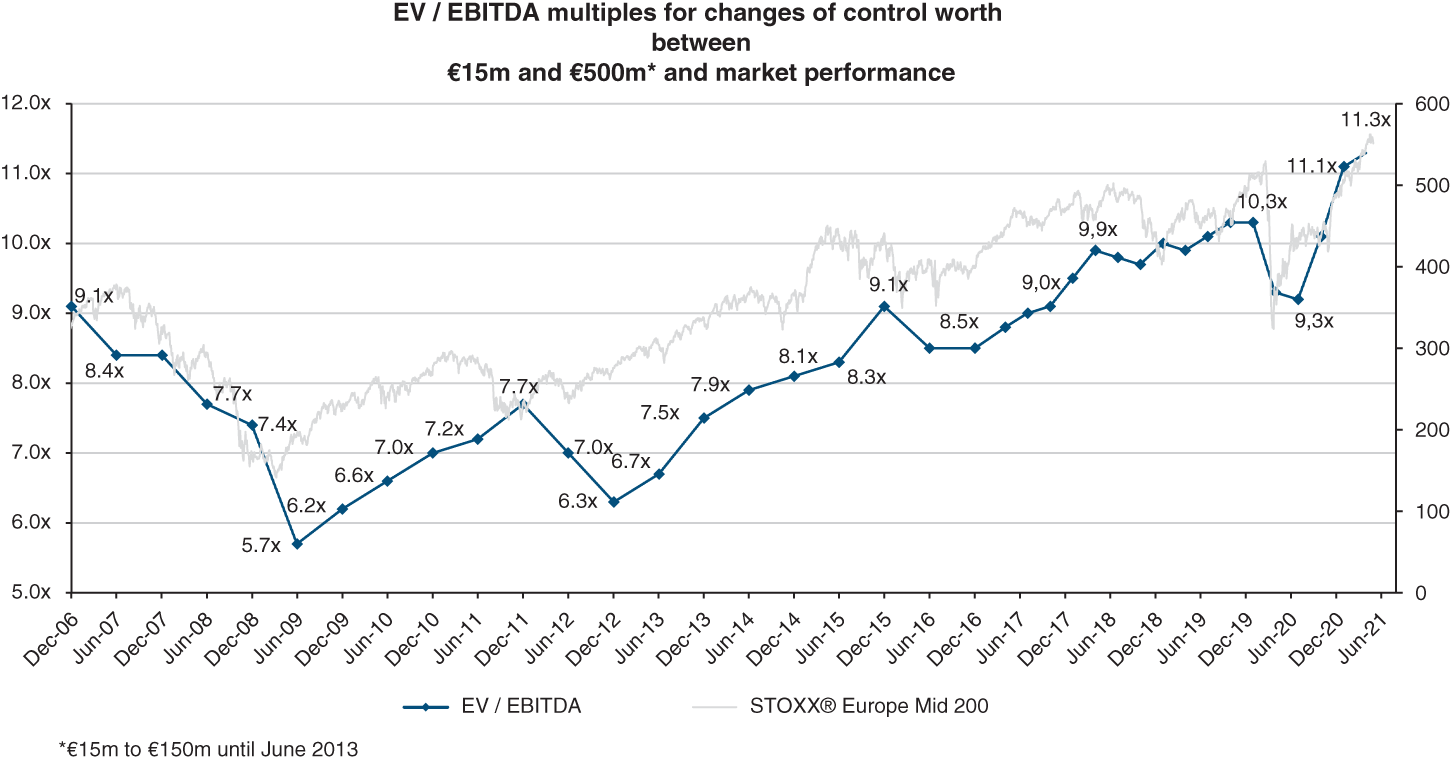
Source: Argos Wityu and Facset
Participants in the market for corporate control think the same way as investors in the financial market. Of course, the smaller the company is, the more tenuous is the link. The value of a butcher's shop or a bakery is largely intangible and hard to measure, and thus has little in common with financial market values. But in reality, only appearances make the market for corporate control seem fundamentally different.
1/ STRATEGIC VALUE AND CONTROL PREMIUM
There is no real control value other than strategic value, which we will develop later. Gone are the days when the control premium was reserved for the majority shareholder and minority shareholders were deprived of it. Stock markets have established equal treatment of shareholders as an absolute principle: minority shareholders are entitled to the same transfer price as the majority shareholder receives for their controlling stake.
Shareholder agreements are a common method for expressing this principle in unlisted companies.
Nevertheless, entrepreneursoften have a diametrically opposed view. For them, minority shareholders are passive beneficiaries of the fruits of all the personal energy the managers/majority shareholders have invested in the company. It is difficult to convince entrepreneurs that the roles of management and shareholders can be separated and that they must be compensated differently – and especially that the risk assumed by all types of shareholders must be rewarded.
If we assume that markets are efficient, then the existence of such a premium can be justified only if the new owners of the company obtain more value from it than its previous owners did. A control premium derives from the industrial, commercial, administrative or tax synergies the new majority shareholders hope to unlock. They hope to improve the acquired company's results by managing it better, pooling resources, combining businesses or taking advantage of economies of scale. These value-creating actions are reflected in the buyer's valuation. The trade buyer (i.e. an acquirer who already has industrial operations) wants to acquire the company so as to change the way it is run and, in doing so, create value.
The company is therefore worth more to a trade buyer than it is to a financial buyer, who values the company on a standalone basis, as one investment opportunity among others, independently of these synergies.
In this light, we now understand that the trade buyer's expectations are not the same as those of the financial investor. This difference can lead to a different valuation of the company. We call this strategic value.
Strategic value is the maximum value a trade buyer is prepared to pay for a company. It includes the value of projected free cash flows of the target on a standalone basis, plus the value of synergies from combining the company's businesses with those of the trade buyer. It also includes the value of expected improvement in the company's profitability compared to the business plan provided, if any.
We previously demonstrated that the value of a financial security is independent of the portfolio to which it belongs, but now we are confronted with an exception. Depending on whether a company belongs to one group of companies or another, it does not have the same value. Make sure you understand why this is the case. The difference in value derives from different cash flow projections, not from a difference in the discount rate applied to them, which is a characteristic of the company and identical for all investors. The principles of value are the same for everyone, but strategic value is different for each trade buyer, because each of them places a different value on the synergies they believe it can unlock and on their ability to manage the business better than current management.
As the seller will also hope to benefit from the synergies, negotiation will focus on how the additional profitability the synergies are expected to generate will be shared between the buyer and the seller.
But some industrial groups go overboard, buying companies at twice their standalone value on the pretext that their strategic value is high or that establishing a presence in such-and-such geographic location is crucial. They are in for a rude awakening. Sometimes the market has already put a high price tag on the target company. Specifically, when the market anticipates merger synergies, speculation can drive the share price far above the company's strategic value, even if all synergies are realised. In other cases, a well-managed company may benefit little or even be hurt by teaming up with another company in the same industry, meaning either that there are no synergies to begin with or, worse, that they are negative, or that the absorption of the company into a much larger group demotivates its managers.
2/ NEGATIVE CONTROL VALUE
Groups can sometimes sell, at a negative price, subsidiaries that are heavily loss-making and that they are unable to turn around. That is, they pay a buyer a sum of money, so that the buyer agrees to buy the shares of that subsidiary from them for a symbolic euro. Thus, in these atypical cases, there is a negative control premium! Materially, the group subscribes to a capital increase of its subsidiary until it reduces its net indebtedness to the negative price agreed with the buyer. Then the transfer of control takes place for one euro.
As the transfer price represents one to three years of losses, from the seller's point of view they have concluded a good financial transaction. Indeed, at a constant loss, the seller recovers their final investment in one to three years, which is a very short payback period. They do not have to carry out a major restructuring or liquidation, which would be damaging to their reputation, especially if they are successful in other sectors.
Following the acquisition for one euro, the buyer will find a net cash position that will enable them to finance part of the company's recovery.
This negative price scenario obviously does not concern listed companies. Thus, in 2021 Saint Gobain sold Lapeyre, which was highly loss-making, to the German turnaround fund Mutares for a negative price of €243m, i.e. 3 times 2020 losses.
3/ MINORITY DISCOUNTS AND PREMIUMS
We have often seen minority holdings valued with a discount, and you will quickly understand why we believe this is unjustified. A “minority discount” would imply that minority shareholders have proportionally less of a claim on the cash flows generated by the company than the majority shareholder. This is not true.
In fact, a shareholder who already has the majority of a company's shares may be forced to pay a premium to buy the shares held by minority shareholders. On average, in Europe, the premium paid to buy out minorities is in the region of 10 to 20% (but the premium can be significantly higher for low liquidity listed companies), less than that paid to obtain control. Indeed, majority shareholders may be willing to pay such a premium if they need full control over the acquired company to implement certain synergies.
Having said that, the lack of liquidity associated with certain minority holdings, either because the company is not listed or because trading volumes are low compared with the size of the minority stake, can justify a discount. In this case, the discount does not really derive from the minority stake per se, but from its lack of liquidity. A minority shareholder, aware of the value of the shareholding it holds, will only be able to sell it if the majority shareholder also decides to sell.
Lack of liquidity may increase the volatility of the share price. Therefore, investors will discount an illiquid investment at a higher rate than a liquid one. The difference in values results in a liquidity discount.
We have encountered some cases where the liquidity discount exceeded 50% for a minority shareholder that wanted to sell its shares, which the majority shareholder only offered to buy after three years of discouraging all potential acquirers. But we have also seen the lack of discount when the disposal of a small stake could change the balance of power in a company.
This is similar to the situation of a listed company with a reduced free float, where the minority shareholder is then in the hands of the majority shareholder who controls the market communication of the firm. Some listed firms can suffer from an undervaluation due to reduced liquidity of the share, so analysts do not publish research and it then becomes a vicious circle.
In a listed company of sufficient size with widely spread capital, the situation is different as the minority shareholder will be protected by the relevant share price and the protection afforded by market authorities.
SUMMARY
QUESTIONS
EXERCISES
ANSWERS
BIBLIOGRAPHY
NOTES
- 1 Earnings before interest, taxes, depreciation and amortisation.
- 2 All the more so as in mature sectors inflation is lower than in the economy in general.
- 3 NOPAT (EBIT after tax) – WACC × Capital employed.
- 4 Including the value of hedging instruments, if any.
- 5 The interest rate calculated as interest in the income statement/net debt in the closing balance sheet does not reflect the actual interest rates paid on the ongoing debt during the year.
- 6 That is, before 1995 in Europe and the US.
- 7 Basel III and IV.
- 8 Which could be the case under IFRS.
- 9 For more on this, see the Vernimmen.com Newsletter no. 24, May 2007.
- 10 Not that of subsidiaries, as it has already been taken into account when valuing the subsidiaries.
- 11 Acquisition of assets will most often generate deductible depreciation whereas acquisition of shares of a company will generate goodwill, which in most European countries does not give rise to tax-deductible amortisation.