
Currency attribution
4.2 Currency attribution returns
4.3 Performance and attribution on unhedged portfolios
4.4 Attribution on an unhedged portfolio
4.8 Naïve attribution on a hedged portfolio
4.10 Brinson attribution on a hedged portfolio
4.11 Problems with the Brinson approach when hedging is active
4.12 Calculating base and return premiums
4.13 The Karnosky-Singer attribution model
4.14 Running Karnosky-Singer attribution on an unhedged portfolio
4.1 INTRODUCTION
Any portfolio with holdings in overseas assets is subject to exchange rate risk. Since most exchange rates fluctuate constantly, such changes may make a substantial contribution to performance, depending on the amounts of overseas assets held and the volatility of the foreign exchange (FX) markets.
This chapter is about ways to measure exchange rate return, the assignment of returns to risks taken and the complications involved when one hedges foreign exchange positions to modify the portfolio’s risk profile.
In previous chapters I introduced the idea of a sector. In this chapter, the only sector used is country or currency.
4.2 CURRENCY ATTRIBUTION RETURNS
So far, I have talked about the return of a security or a portfolio as a single quantity. When currency exposures are active, there are two types of return to consider instead of one:
- Local currency return: the return of an asset expressed in the home, or local, currency of the asset. All returns described so far are local currency returns.
- Base currency return: the return of an asset expressed in the base, or denominating, currency of the portfolio. For instance, if an asset is denominated in GBP but the portfolio in which it is held is denominated in USD, then it will have two measures of return: a local currency GBP return and a base currency USD return.1
Assuming continuous compounding, the base currency return rBASE of an asset is given by
where rLOCAL is its local currency return, and rFX is the foreign exchange return due to changes in the exchange rate between the local and base currencies.
For example, suppose that you have US dollars to invest. Your research tells you that over the coming year the prospects for the Indonesian stock market are particularly good, but there is a significant risk that the Indonesian rupiah will devalue against the US dollar during the same period.
Nevertheless, you convert your dollars into rupiah and purchase Indonesian stock. Should the Indonesian stock market go up 10% (the local currency return), but the value of the rupiah drop 20% over the same interval (the foreign exchange return), then the base currency return of your investment is 10% − 20% = −10%. The overall result is a loss, even if you were right about the gains to be made in the Indonesian market.
4.3 PERFORMANCE AND ATTRIBUTION ON UNHEDGED PORTFOLIOS
Consider the following AUD-denominated portfolio, which has exposure to several foreign currencies. In Table 4.1 the columns show, in order: country, portfolio weights (wP), local portfolio returns ![]() benchmark weights (wB), local benchmark returns
benchmark weights (wB), local benchmark returns ![]() and benchmark return from exchange rate movements (rFX) over the calculation interval.2
and benchmark return from exchange rate movements (rFX) over the calculation interval.2
Table 4.1 Weights and returns for demonstration portfolio

The aggregate local currency returns for portfolio and benchmark are shown at the bottom of the third and fifth columns. Note that the difference between these figures is not the actual active portfolio return, as they ignore the impact of exchange rate shifts.
While base and local currency returns are often different, base and local currency weights are always the same, as their relative holdings are unchanged no matter how return is measured. For this reason, we use a single measure of weight when calculating local and base currency portfolio returns.
The true active return of the portfolio is calculated by comparing the base currency returns ![]() and
and ![]() for each country. These are derived by summing the local currency returns
for each country. These are derived by summing the local currency returns ![]() and
and ![]() with the exchange rate return rFX over each sector, as shown in Table 4.2.
with the exchange rate return rFX over each sector, as shown in Table 4.2.
Table 4.2 Base currency returns
| Country | ||
| Germany | 6.80% + 1.00% = 7.80% | 7.00% + 1.00% = 8.00% |
| UK | 12.25% − 3.00% = 9.25% | 10.50% − 3.00% = 7.50% |
| Japan | 10.50% − 1.00% = 9.50% | 9.50% − 1.00% = 8.50% |
| Australia | 9.00% + 0.00% = 9.00% | 8.40% + 0.00% = 8.40% |
| Cash | 8.00% + 0.00% = 8.00% | 7.50% + 0.00% = 7.50% |
| Total | 8.305% | 8.100% |
The base currency returns for portfolio and benchmark are given by the sum-product of the country weights with the corresponding base currency country returns:

The true overall outperformance, in base currency terms, is therefore 8.305% − 8.100% = 0.205%.
To see this result in a different way, treat the portfolio as two subportfolios; one with exposure to local markets, but no exposure to currency; and another with no local market component, but exposure to currency movements.
- The local contribution to return for the portfolio is 8.105%.
- The local contribution to return for the benchmark is 8.850%.
- Currency return from the portfolio is (60% × 1%) + (10% × −3%) + (10% × −1%) + (0% × 9.00%) + (0% × 8.00%) = 0.200%.
- Currency return from the benchmark is (25% × 1%) + (25% × −3%) + (25% × −1%) + (25% × 0%) + (0% × 0%) = −0.750% .
The overall portfolio return is 8.105% + 0.200% = 8.305%. The overall benchmark return is 8.850% − 0.750% = 8.100%. The active outperformance is 0.205%, as before.
If a security is denominated in the portfolio’s base currency return, its local and base currency returns will be identical and it will not generate FX returns. For instance, the example portfolio above is denominated in AUD, so the FX returns from its AUD holdings were zero.
4.4 ATTRIBUTION ON AN UNHEDGED PORTFOLIO
Just as for a single-currency portfolio, we can run attribution on a portfolio with foreign exchange exposures to decompose its active returns by sources of risk.
One way to do this is to convert everything to base currency returns and run standard Brinson attribution, using
for the asset allocation return of sector S, and
for the stock selection and interaction return of the same sector, where ![]() are the weights and base currency returns of sector S in portfolio and benchmark, respectively, and rB is the base currency return of the benchmark. These expressions give the results shown in Table 4.3.
are the weights and base currency returns of sector S in portfolio and benchmark, respectively, and rB is the base currency return of the benchmark. These expressions give the results shown in Table 4.3.
Table 4.3 Brinson attribution using base currency returns
| Country | rAA | rSS |
| Germany | −0.035% | −0.120% |
| UK | 0.090% | 0.175% |
| Japan | −0.060% | 0.100% |
| Australia | −0.030% | 0.090% |
| Cash | −0.030% | 0.025% |
| Subtotal | −0.065% | 0.270% |
| Total | 0.205% |
Although correct, this analysis does not separate the returns generated by exchange rate movements from asset allocation and stock selection returns. For a clearer view of the effects of the manager’s investment decisions, one should treat this multi-currency portfolio as two subportfolios, one containing securities with returns measured in local currency and one containing FX positions. This allows the value added by local currency investment decisions to be separated from the value added by exchange rate movements.
For the example shown in Table 4.1, the local currency asset allocation return for sector S is again given by the standard Brinson expression
and the local currency stock selection return by
where the weights have the same definitions as above, but the returns are now in local currency terms.
When running Brinson attribution on currency holdings, the FX return of portfolio and benchmark sectors is always the same, so the stock selection term will always be zero.3 For this reason we do not show a stock selection return for the portfolio’s foreign exchange exposure, and instead use
for the currency asset allocation return, where ![]() is the FX return of country S, and rFX is the benchmark’s FX return, given by
is the FX return of country S, and rFX is the benchmark’s FX return, given by
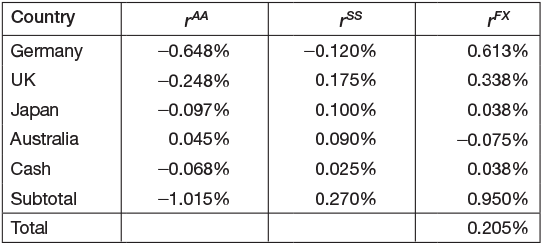
For instance, the attribution and stock selection returns for Germany are as follows:
rAA = (60% − 25%) × (7.000% − 8.850%) = −0.648%
rSS = 60% × (6.80% − 7.00%) = −0.120%
rFX = (60% − 25%) × (1% − 0.750%) = 0.613%
where all values are taken from Table 4.3. Overall, the results are as shown in Table 4.4.
Table 4.4 Brinson attribution using local and FX returns
This approach to running attribution on a multi-currency portfolio is called naïve attribution – not because it is wrong, but because it omits some important factors that can affect attribution when we hedge a portfolio.
4.5 PORTFOLIO HEDGING
Although the returns to be made in overseas investments might look attractive, the portfolio manager may not want to take the associated currency risk by investing in assets that have exchange rates that may move against them.
Fortunately, there are ways to remove this currency risk, albeit at a cost. A technique called hedging involves holding additional securities that have an equal and opposite currency exposure to the assets held in the portfolio. If the exchange rate falls, the value of the hedge security will rise by an equal amount, so the net effect on the hedged asset’s return from the change in exchange rates will be zero.
A portfolio that has holdings in overseas assets automatically has exposure to exchange rates. However, by using hedging we can change the exchange rate exposure to anything we want.
4.6 CURRENCY FORWARDS
One way to hedge foreign exchange exposures is to use a forwards contract.4 A forwards contract is simply an agreement to exchange two currencies for a given length of time. In effect, we borrow one and lend the other, paying interest on the first and receiving interest on the second. The cost of the contract depends on the length of time for which the currencies are to be exchanged and their respective interest rates, but the net result is that, for the period during which the forwards contract is active, one has an additional FX exposure.
Forwards are usually traded in terms of a forward exchange rate. However, for attribution on hedge positions it is more useful to consider the cost of the contract in terms of the underlying interest rates.
A forwards contract always has a known expiration date. If the portfolio manager wishes to keep a currency hedge in place after this date, they enter into a new agreement with a counterparty. This is called rolling the contract.
Example: hedging Indonesian rupiah into US dollars
Consider the earlier example of buying Indonesian rupiah (IDR)-denominated securities with USD.
At the same time that the trader converts their US dollars into Indonesian equities, they take out a forward position in USD against rupiah so that the positive IDR exposure in stocks is offset by a negative IDR exposure in the forward contract.
In other words, the trader has bought IDR securities, so has an IDR currency exposure. To eliminate this exposure the trader needs to sell some other IDR and buy USD. This can be done by:
- borrowing IDR, and paying the Indonesian interest rate on the amount borrowed;
- buying USD, and receiving the USD interest rate on the same amount.
This aggregate position (short IDR, long USD) is the forward hedge. At the time of writing the IDR interest rate is much higher than the USD (5.75% vs 0.25%); so it only makes sense to follow this strategy if the expected annual return from investing in Indonesia exceeds the interest rate differential between the two countries (5.75% − 0.25% = 5.5%). The difference is called the cost of hedging.
However, suppose the trader goes ahead with this strategy. If the IDR falls, then the decrease in the value of the stocks due to this exchange rate movement will be exactly offset by an increase in the value of the forward hedge. The net impact of the change in exchange rates will be zero. The trader will still benefit from any returns in IDR stocks in local terms, although there will be a hedging cost of 5.5% of the exposure to pay. Therefore, this strategy only makes sense if the expected annual returns of the underlying asset exceed 5.5%.5
It is possible to hedge only part of a position. For instance, one might want to keep a partial exposure to the IDR in order to benefit from any appreciation in the currency. In this case, one might hedge only 50% of the exposure, at half the cost of the full hedge.
4.7 HEDGING AND RISK
The reasons why one might hedge can vary widely. In addition to removing risk, one may also seek to add it.
- A defensive or hedging strategy involves taking as little FX risk as possible. A perfect hedge is one that reduces FX risk to zero.
- An active or speculative strategy involves the active taking of risks in addition to the equity selection decisions, for instance, by seeking to profit from an expected forthcoming change in exchange rates.
- A mixed strategy involves a combination of defensive and active risks. For instance, the manager might seek to hedge away currency risk in most areas, but to take a small number of active currency bets for selected countries.
- A portfolio may need to be hedged if its benchmark is also hedged, to ensure that the same constraints are followed.6
Exchange rate strategy often is seen as a specialised area of expertise, since managers who specialise in asset allocation or stock selection may prefer not to manage currency exposures as well. For this reason, currency decisions are often outsourced to ‘currency overlay’ managers (Record, 2003).
4.8 NAÏVE ATTRIBUTION ON A HEDGED PORTFOLIO
The approaches described so far can also be used to analyse the returns of a hedged portfolio.
A hedged portfolio is essentially three portfolios in one: a portfolio with local returns generated by changes in the local prices of its constituent securities, another portfolio driven by returns generated by exchange rate movements and a third portfolio of hedging instruments. By allowing hedging, we have decoupled the currency allocation decision from the asset allocation and stock selection decisions.
Suppose that the portfolio shown in Table 4.1 has been hedged using currency forwards to give the exposures shown in Table 4.5. The second column C shows the hedge position. This is the actual currency exposure of the portfolio, as distinct to its market exposure. The third column F shows the forward positions required in each currency to give the net hedge, given the portfolio’s physical exposures.
Table 4.5 Weights and returns for demo portfolio

To ensure the currency exposures are as shown, set up forwards positions equal to the hedge position, minus the portfolio position. For instance, the UK’s hedge exposure is 10% in the portfolio, but the securities held in the portfolio contribute 55%. Therefore the UK forward position is 10% − 55% = − 45%.
The hedging comes at a cost. Since we are borrowing in some currencies and lending in others, there are interest payments involved, which will affect the returns of the various positions in the portfolio. Therefore, the base currency return of a hedged asset from a given country will be affected by:
- its local currency return;
- the return generated by changes in exchange rates;
- the interest (or cash) rate of the local currency;
- the interest (or cash) rate of the base currency.
Without hedging, the portfolio’s currency exposure is exactly the same as its market exposure. The portfolio has no hedge currency exposures, so interest rates do not enter into the returns calculation.
With hedging, the market exposure can differ from the currency exposures. The portfolio’s return is now driven by a combination of market returns, FX movements and cash returns.
4.9 MEASURING HEDGE RETURNS
A country’s return from interest ![]() is the active weight
is the active weight ![]() of that country in the hedge, times the cash rate
of that country in the hedge, times the cash rate ![]() for that country:
for that country:
Active weight is measured relative to the portfolio, not the benchmark, since it is the portfolio that is hedged, not the benchmark. The active weight ![]() of the hedge is given by
of the hedge is given by
where ![]() is the portfolio hedge weight and
is the portfolio hedge weight and ![]() is the portfolio market weight in the portfolio.
is the portfolio market weight in the portfolio.
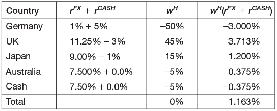
For this portfolio, return due to movements in FX rates is given by (−50% × 1%) + (45% × −3%) + (15% × −1%) + (−5% × 0%) + (−5% × 0%) = −2.00% while return due to hedging exposures is (−50% × 5%) +(45% × 11.25%) + (15% × 9%) + (−5% × 7.5%) + (−5% × 7.5%) = 3.163% (see Table 4.6). The second and third columns are the returns in local terms, as before. The fourth (Local) column is the cash return, or the interest earned by holding exposures in these currencies. The contribution from each country is the active hedge weight for that country, times the return of that country’s currency. The fifth (FX) column is the FX return times the active hedge weight.
Table 4.6 Returns of hedged portfolio

The overall active return of the hedged portfolio is therefore given by rP − rB = 8.305 − 8.100 + 3.163 − 2.000 = 1.368.
To view the value added by the hedged currency position, examine the individual performance contributions in Table 4.7.
Table 4.7 Performance contributions from currency
4.10 BRINSON ATTRIBUTION ON A HEDGED PORTFOLIO
The results from the earlier attribution without the hedge in place can now be combined with the results shown in Table 4.7 to give the overall Brinson attribution.
The presence of the new hedge makes no difference to the local currency asset allocation and stock selection returns. Currency hedging only gives rise to asset allocation returns, since the stock selection returns are identical for portfolio and benchmark. Table 4.8 shows the results of combining Tables 4.4 and 4.7.
Table 4.8 Brinson attribution using local and FX returns

4.11 PROBLEMS WITH THE BRINSON APPROACH WHEN HEDGING IS ACTIVE
An issue with applying this attribution model to hedged portfolios is that its results are not always consistent with intuition.
Recall that Table 4.4 showed the results of overweighting Germany (60% vs 25%) in an unhedged portfolio. Germany underperformed in local currency terms (7.00% vs 8.85%), so the Brinson approach indicates that overweighting Germany was a bad decision, and generated an active return of −0.648%.
However, if we allow hedging the situation becomes more complex. In addition to the local sector returns and the FX returns, hedging also generates extra cost and benefits due to the availability of additional interest rate exposures.
In fact, hedging can fundamentally change the outcome of this analysis because it alters the average level of return. Without hedging, the return from a non-base currency position is
When hedging from one currency to another is available, the return from a hedged position becomes
To illustrate the extra opportunities that can arise when hedging is available, consider the highest return that could have been made on the sample portfolio in Table 4.1.
Without hedging, the best strategy would have been to invest entirely in Japanese equities for a return of 10.50% local return − 1% FX return = 9.5% base return.
Suppose instead that we bought German equities and simultaneously hedged out of Deutsche Mark (DEM) and into GBP. In this case, the return would have been the sum of:
- 6.80%: Local currency return made by investing in Germany;
- 11.25%: Interest made on UK cash holdings via the hedge contract;
- −5%: Interest paid on DEM cash borrowings via the hedge contract;
- −3%: FX movements,
which totals 10.25%, substantially more than the 9.5% to be made by investing in unhedged assets.
The interplay between local return, FX return, and the interest returns paid or received from the various hedging currencies can make it difficult to see the best combination of local markets and hedging strategy. For this illustrative portfolio, a list of all possible investment and hedging strategies is shown in Table 4.9, sorted in descending order of net return, which shows that the strategy we used earlier as an example (buy German equities, hedge into GBP) was in fact the best possible.

The moral is that with the ability to hedge, the range of possible outcomes changes. The reference return that the manager should be trying to beat is no longer the average unhedged return, but the average hedged return – which can be quite different.
By allowing hedging, we have moved the goalposts. Unless all interest rates are the same across all currencies, there will be combinations of markets and hedging positions that will give higher returns than those available from the original range of unhedged markets. The availability of these new opportunities should be reflected when we come to measure the manager’s skill.
In particular, Table 4.9 shows that, once the ability to hedge exposures is taken into account, overweighting Germany should have been regarded as a good decision. This is not reflected in the results based on the naive approach, which suggests the exact opposite.
4.12 CALCULATING BASE AND RETURN PREMIUMS
A simple transformation makes it straightforward to work out which investment strategy gives the best hedged returns, without considering every individual case.
- Instead of using local currency return, replace rlocal with rlocal – rcash when calculating asset allocation returns. This quantity is called the local return premium (or just the return premium).
- Instead of using FX return, replace rFX with rFX + rcash. This quantity is called the hedged Eurodollar rate (or the base return).7
To see why this makes sense, consider where our returns come from when local market positions and currency exposures can be managed separately.
- The true return made from holding a currency is its FX return, plus the interest payable on that currency. This is the return generated by holding assets in a particular country without making any investment decisions.
- The true return from holding a market exposure is that market’s return, minus the interest payable to holding an exposure in that currency. This is the excess, real return one gains from investing in a market, over and above the risk-free rate.
Therefore, the appropriate returns to use for performance and attribution of hedged portfolios are the return premium and the base return, rather than the local market and FX returns.
Suppose that a position is unhedged. In this case, the FX exposure will be the same as the market exposure. The return for each market is then simply the local return plus the FX return, since the cash rates cancel out.
In Table 4.10, Base return is given by rCash + rFX and Return premium by ![]() All totals are averaged using benchmark weights.
All totals are averaged using benchmark weights.
Table 4.10 Sector-level and aggregated adjusted returns

By inspection, the highest possible local return is made by investing in Germany (2%) since this the largest available figure in the Return premium column. Similarly, hedging into GBP gives the highest base return of 8.25%, since this is the largest figure in the Base return column.
Together, the active return from the combination of both strategies is 2% + 8.25% = 10.25%. Similarly, the lowest return is made by investing in the UK (−0.75%) and hedging into DEM (6%) giving an active return of 5.25%. Both results are consistent with Table 4.9.
The ability to hedge into other currencies, and transfer currency risk, can increase the opportunities available to increase return, and this should be acknowledged in any attribution analysis. The technique was introduced in a seminal 1994 monograph by Dennis Karnosky and Brian Singer (Karnosky and Singer, 1994).
The core insight behind Karnosky and Singer’s approach to hedged currency attribution is that spot exchange rates are insufficient to decide whether currency decisions in a hedged portfolio were successful.
Instead, if we use (local currency return) minus (cash rate) as the return in an asset allocation calculation for country exposure, and (FX return) plus (cash rate) as the return in an asset allocation calculation for FX return, then the results will reflect the merit (or otherwise) of the various investment decisions made when the ability to hedge is taken into account.
For instance, in our demo portfolio we were overweighting Germany, which we now know to have been a good decision when the portfolio can be hedged. The local return premium for Germany was 7% − 5% = 2%, which is greater than the average local return premium of 0.66%. So this position added (60% − 25%) × (2.00% − 0.66%) = 0.468, rather than the −0.648% indicated by the earlier approach.
4.13 THE KARNOSKY-SINGER ATTRIBUTION MODEL
A formal statement of the Karnosky-Singer algorithm is given in Appendix A, but the results applied to the sample hedged portfolio in Table 4.5 are shown in Table 4.11.
Table 4.11 Results of Karnosky-Singer attribution

To illustrate the calculation, consider Germany.
- Market asset allocation return rAA is

where ![]() is the return premium for sector S, and
is the return premium for sector S, and ![]() is the sum-product of the benchmark weights and the return premiums, given in Table 4.10.
is the sum-product of the benchmark weights and the return premiums, given in Table 4.10.
- Stock selection return rSS is
- Currency allocation return rFX is

where ![]() is the base premium for sector S, and
is the base premium for sector S, and ![]() is the sum-product of the benchmark weights and the base premiums – also read from Table 4.10.
is the sum-product of the benchmark weights and the base premiums – also read from Table 4.10.
4.14 RUNNING KARNOSKY-SINGER ATTRIBUTION ON AN UNHEDGED PORTFOLIO
The Karnosky-Singer framework can be applied to both hedged and unhedged portfolios. If no hedging is in place, the calculation reduces to the unhedged approach. There is, therefore, no theoretical penalty in implementing this model for routine attribution, although the Karnosky-Singer approach has extra data requirements (a cash return for each market) while the naive approach does not.
1 In the fixed income world it is quite common for bonds issued by one country to be denominated in the currency of another. The generic term for such a security is a Eurobond.
2 This data is intentionally identical to that provided in the monograph by Karnosky and Singer (1994) and Laker (2003), to allow the approaches of different authors to be compared.
3 An exception to this can occur if different FX revaluation rates are used for portfolio and benchmark. Returns from this effect are covered in Chapter 2 under the section ‘Price return’.
4 Other alternatives include the use of currency swaps, currency futures contracts and currency options.
5 The counterpart to this strategy is a carry trade. As long as exchange rates do not change, a trader can make a profit by buying a (risky) high-yielding currency and selling a (safer) low-yielding one.
6 Many data suppliers supply customised hedged benchmarks to match the investment mandates of their customers. While the constituents and overall returns of the benchmarks are supplied, it is relatively rare for the hedges to be published. This is a considerable nuisance for attribution analysts, who need to know all the security exposures in both portfolio and benchmark in order to run attribution. Appendix B shows one way around this problem.
7 I find these terms confusing, but mention them here so that you can follow other literature on this topic.