There has been a lot of progress on the R Markdown development since the first edition of this book. To make it clear, there are two versions of R Markdown: we call the implementation in the markdown package (Allaire et al., 2015b) “R Markdown v1” (https://github.com/rstudio/markdown), and we call the implementation rmarkdown (Allaire et al., 2015a) “R Markdown v2” (http://rmarkdown.rstudio.com). Unless otherwise noted, use of the term “R Markdown” in this chapter refers to R Markdown v2.
R Markdown v1 is based on the C library sundown, and the major focus is HTML output. Its functionality is very limited, e.g., there is no support for citations or footnotes. R Markdown v2 is based on Pandoc, which has boosted Markdown to a whole new level. There are two aspects of the improvements: the Pandoc Markdown syntax is richer, so we can write more types of elements, and the output format is no longer limited to HTML —we can also export Markdown to ![]() /PDF, Word, and HTML5 slides, etc. In this chapter, we will introduce the design philosophy of rmarkdown, what it can do, and how to customize or extend it.
/PDF, Word, and HTML5 slides, etc. In this chapter, we will introduce the design philosophy of rmarkdown, what it can do, and how to customize or extend it.
Although knitr supports a variety of document formats (Chapter 5), R Markdown is probably the most popular one. Markdown, limited as it is in terms of functionality, is a nice document language for beginners. On the other hand, authors may not even want a lot of features at all. Markdown may be restrictive in the eyes of ![]() users, but not everyone needs to care that much about typesetting details.
users, but not everyone needs to care that much about typesetting details.
The limitation of Markdown can be largely removed by Pandoc, but the problem is that Pandoc is a command-line tool. Power users may not find this to be a real problem, but the large number of command-line arguments can be overwhelming to beginners.
The goal of rmarkdown and R Markdown v2 is to provide quick conversion of R Markdown files into other document formats, using reasonably beautiful templates. The way that we achieve the goal is to wrap commonly used command-line arguments into R functions in rmarkdown. The main function in rmarkdown to render R Markdown documents to other document formats is render(). The first argument is the Rmd filename, and the second argument is the output format, which we will introduce in detail later in this chapter. For example, if you want to convert an R Markdown document foo.Rmd to Word, you only need to execute one line of code:
![]()
You can certainly do it the hard way: first, call knit() in knitr to compile foo.Rmd to foo.md; then open a terminal or use the R function system() to execute a command like this, as we introduced in Section 13.2:

There are seven output format functions in rmarkdown at the moment: PDF, HTML, Word, Markdown, ioslides, Slidy, and Beamer. The first four are document formats, and the latter three are presentation formats. They are wrapper functions for both knitr and Pandoc, so you do not need to remember a lot of knitr options and Pandoc arguments — knitr chunk options and Pandoc command-line arguments are converted to rmarkdown function arguments. For example, the Pandoc argument --toc or --table-of-contents corresponds to the function argument toc = TRUE in rmarkdown.
In addition, rmarkdown has provided its own templates that aim to be visually pleasing by default. For example, for HTML output, it uses the Twitter Bootstrap styles and themes. Syntax highlighting for program code is also enabled by default.
The rmarkdown package is well supported in the RStudio IDE: you do not need to manually call the render() function, and you only need to click the Knit button on the toolbar. You can also set the output format and its options from a little GUI popped up through the gear button on the toolbar. If you wish to run rmarkdown outside of RStudio, you will want to learn more details about how rmarkdown works later.
Note RStudio has embedded Pandoc in it, so you do not need to install Pandoc separately if you use RStudio, otherwise you need to install Pandoc by yourself. If you have a separate installation of Pandoc, RStudio will use it only if your version is higher than RStudio’s Pandoc version.
14.2 Pandoc’s Markdown Extensions
First we introduce the syntax of Pandoc’s Markdown. If you are familiar with R Markdown v1, you can still use its syntax with Pandoc, and the only significant change is how to write superscripts that are not math elements. In v1, you use a single caret, e.g., xˆ2. In Pandoc’s Markdown, you need to surround the superscript with ˆ, e.g. xˆ2ˆ. For math expressions, you still use one caret, e.g., $xˆ2$.
The syntax for other elements remains more or less the same in Pandoc’s Markdown. For example, you use one # sign to write the first level section header, and two # signs for the second level header. Please review Section 5.2.1 for the syntax of basic elements in Markdown. Below are some new elements that may be useful (see http://johnmacfarlane.net/pandoc/ for the full documentation), and we show short examples of these elements under the bullets:
• Definition lists and example lists

• Footnotes using ˆ[…] and citations using [@id]

• Figure/table captions

• Raw ![]() /HTML content
/HTML content


When using citations, you need to specify a bibliography database. If you are familiar with ![]() , you are likely to know Bib
, you are likely to know Bib![]() as well. The bibliography database can be a
as well. The bibliography database can be a .bib file specified in the bibliography field in the YAML metadata (see next section). If you do not know Bib![]() , you can embed the bibliography items in the YAML metadata using the
, you can embed the bibliography items in the YAML metadata using the references field (instead of bibliography), e.g.,

Except for raw ![]() /HTML code, all other elements are portable across all document formats. For example, a footnote
/HTML code, all other elements are portable across all document formats. For example, a footnote ˆ[foo bar] will be converted to footnote{foo} when the output format is ![]() , and something like
, and something like <a href="#footnote-1"><sup>1</sup></a> with the link target footnote-1 being a footnote item at the bottom of the page when the output format is HTML. You should not expect raw ![]() in Markdown to be converted perfectly to Word, or raw HTML to be converted to Beamer, since raw
in Markdown to be converted perfectly to Word, or raw HTML to be converted to Beamer, since raw ![]() and HTML content can be fairly complicated, and perfect conversion is nearly impossible.
and HTML content can be fairly complicated, and perfect conversion is nearly impossible.
Another important extension in Pandoc’s Markdown is the YAML metadata. YAML stands for “YAML Ain’t Markup Language” or “Yet Another Markup Language,” and it is basically a nested list structure. Pandoc uses YAML to write metadata of a document, such as the title, author, and date information. The metadata usually appears in the beginning of a document, and is enclosed between two lines of three dashes ---. Typical YAML metadata looks like this:

The most important field in the YAML metadata for rmarkdown is the output field. This is where we specify the desired output format. If it is missing, rmarkdown will assume the output format to be an HTML document. If multiple formats are specified, the render() function will use the first format by default, unless you have specified the second argument of render() explicitly. You can also use render(’foo.Rmd’, ’all’) to render all formats defined in the output field.
There is a series of format functions in rmarkdown with the suffixes _document and _presentation, e.g., html_document(), pdf_document(),and beamer_presentation(), etc. These functions can be used as the second argument of render(), e.g.,

Each output format function has its own arguments. For example, if you want to enable the table of contents for an HTML document, you can call:
![]()
This is equivalent to providing the YAML metadata as:
In YAML, both yes and true mean the logical value TRUE. You can either use the YAML metadata and call render() without the second argument, or omit/ignore the YAML metadata and provide the second argument explicitly to render(). The YAML approach is more convenient and common; the output information is contained in the source document. The second approach can be useful when you want to override the output formats defined in YAML. See the help page of each output format function for what the possible options are, e.g., type ?rmarkdown::pdf_document in the R console to see the options for PDF output.
An output format function returns a list of options, including knitr package/chunk options, Pandoc arguments, and other auxiliary options for rmarkdown. We will explain them using html_document() as the example.
To see what html_document() really returns, you can run it and print the structure of the object returned:

As you can see, html_document() has modified some of the knitr default chunk options, such as fig.height (knitr’s default is 7), and fig.retina (the original default is 1). These changes are for aesthetic reasons, although it is somewhat subjective to decide what kind of option values give better-looking results.
The list also contains Pandoc options: the output format is html, as you can see in the element pandoc$to; a few Pandoc arguments such as --smart and --self-contained are also included in the list.
There are some auxiliary options for rmarkdown, too. For example, clean_supporting means whether to clean up the intermediate output files after the HTML file has been rendered. Intermediate files may include figure files: if you want the HTML file to be self-contained, Pandoc will embed all external resources in it (such as images), so you no longer need these external files. In that case, render() will delete them after rendering the HTML file.
After we know the internals of an output format function, we can write our own format functions using different knitr/Pandoc options. We will introduce how to implement custom formats later in this chapter.
Now we show a full example of an R Markdown v2 document named Rmd-v2.Rmd. It is a little bit long, but it shows most of the features of Pandoc and rmarkdown.


FIGURE 14.1: A preview of the HTML output document from R Markdown v2 in an RStudio window.

You may need to review the sections 6.3 and 12.4.1 if you are not sure about how kable() or write_bib() works.
Figure 14.1 is a preview of the HTML output document after we render this example in RStudio. It shows the title, author, date, and the first few sections of the document. That is the default Twitter Bootstrap style in rmarkdown. Figure 14.2 is a preview of the last few sections. Even though footnotes and citations are not native elements of HTML (they may be natural to ![]() users), Pandoc managed to generate them in HTML anyway.
users), Pandoc managed to generate them in HTML anyway.
There is a large number of options that you can tweak for the HTML output. See the help page ?rmarkdown::html_document for a full list.

FIGURE 14.2: A preview of the table, footnotes, and citations: the table was generated by kable(), and the bibliography database was created from write_bib() in knitr.
For example, we change the CSS theme using the theme field, add a table of contents using the toc field, and number the section titles using the number_sections field in YAML (Figure 14.3):

Currently these CSS themes are available in rmarkdown (you can see a preview at http://bootswatch.com):
![]()
If you need to further tweak the appearance of the output, you can apply your own CSS files using the css field, e.g.,

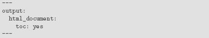
If you just want to use your own CSS and do not want any themes (including syntax highlighting themes) from rmarkdown, you can remove them completely by specifying theme and highlight to be null:
Because an HTML page often has external dependencies, such as CSS, JavaScript, and image files, it may be inconvenient when you share the HTML file with other people, because you have to make sure these dependencies are also included when you send the HTML file to them. Pandoc has an option to make the HTML file self-contained by embedding all external dependencies into the HTML file. For example, JavaScript files are read into the HTML file, and images are base64 encoded. You can share a self-contained HTML file just like a PDF file; everything you need has been embedded into a single file. In rmarkdown, this is controlled by the option self_contained. When you have multiple Rmd files to be rendered by rmarkdown, it may be a good idea to turn off the self-contained mode, otherwise there will be a lot of redundancy since some external dependencies may be embedded into every single HTML output file. When the self-contained mode is off, you can put the shared dependencies into a common directory, specified via the lib_dir option, e.g.,

FIGURE 14.3: A preview of the “readable” theme (you can see the fonts are different with Figure 14.1), with a table of contents and numbered sections.

Sometimes you may want to include additional content in the HTML header, before the body, or after the body of the document. In these cases, rmarkdown has an option includes in which you can specify the filenames of the additional content. Suppose you want to use the JavaScript library D3 (http://d3js.org) in the HTML output, then you can write this in a file doc_header.html:
![]()
You also have two files doc_before.html and doc_after.html, which are the content to be inserted before and after the body, respectively. For example, you may want to write a navigation menu in doc_before.html, and some copyright information in doc_after.html. These three files can be included in the HTML output file by:

For any output format, Pandoc needs a template to create the output file. There are several Pandoc variables available in the template, and you can use these variables to define your own template. For example, this can be a minimal HTML template:

We only used two variables $title$ and $body$ in this template. The first variable contains the document title specified in the title field in the YAML metadata. The second variable is the body of the Markdown document after it is converted to HTML. You can learn more possible variables from either the rmarkdown source package (https://github.com/rstudio/rmarkdown) or Pandoc’s default templates (https://github.com/jgm/pandoc-templates).
To use a custom template, you can use the template field in YAML, e.g.,

Finally, you can customize command-line arguments to be passed to Pandoc in the pandoc_args field. As a matter of fact, the R arguments in html_document() are eventually converted to Pandoc arguments. For example, the R argument self_contained = TRUE (or self_contained: yes in YAML) is equivalent to the Pandoc argument --self-contained, and also equivalent to this in YAML:

So far we have covered most of the possibilities to customize the output on the Pandoc’s Markdown side. It is also possible to customize knitr chunk options in YAML. Currently there are four chunk options that you can set in YAML:
fig_width, fig_height the default size of the figures
fig_retina a scaling ratio for Retina displays; the default is 2 in rmarkdown, which means a figure of the size m × n has an actual size of 2m × 2n, but is scaled to half of its actual size in the output (this can improve the image qualities on Retina displays)
fig_caption whether to render and show figure captions (this basically means the figure environment with caption{} when the output format is ![]() ); if
); if FALSE, you will not see the figure caption in HTML output, since the caption will be put in the alt attribute of the <img> tag, which is invisible
Apparently, the fig_retina option will make the file size of images larger in return for the image quality. You can try fig_retina = TRUE and FALSE separately, and see if you can notice any differences on your device.
Once you are familiar with the HTML document format, it will be easy for you to master other output formats, because many options are common in these formats. For example, you can also use the options such as fig_width, fig_height, toc, number_sections, and highlight in pdf_document(). In this section, we only focus on the options that are specific to PDF document output.
Figure 14.4 is a preview of a page in the PDF output from the same example we used in the previous section. It does not look too much different from Figure 14.2. For the same R Markdown document, everything that worked in the HTML output still works in ![]() /PDF, including section headings, tables, footnotes, and citations, etc.
/PDF, including section headings, tables, footnotes, and citations, etc.
Similarly, we can add a table of contents, and number the sections as we did for the HTML output (Figure 14.5):


FIGURE 14.4: A preview of the 4th page of the PDF output document from the R Markdown v2 example.

FIGURE 14.5: A preview of the PDF output document, with a table of contents and numbered sections.
Pandoc has a few ![]() -specific options that you can use in the YAML metadata, and you can find the full documentation on the Pandoc website. We only list a few of them here:
-specific options that you can use in the YAML metadata, and you can find the full documentation on the Pandoc website. We only list a few of them here:
fontsize the font size of the document, e.g., 10pt, 11pt, 12pt
documentclass the document class, e.g., article, book, report
classoption options for the document class, e.g., a4paper, twocolumn
geometry options for the geometry package, e.g., tmargin=2cm, bmargin=2cm, lmargin=3cm, rmargin=3cm
Note these are top-level options in YAML, and you should not put them under the pdf_document field.
The default ![]() engine is pdflatex, and you can change it via the latex_engine option in pdf_document(). Currently possible engines are
engine is pdflatex, and you can change it via the latex_engine option in pdf_document(). Currently possible engines are pdflatex, xelatex, and lualatex. You may also preserve the intermediate ![]() output file via the
output file via the keep_tex option, which can be useful for debugging and other purposes.
Below is an example of the YAML metadata for a document that uses the book class, a font size of 11pt, a two-column layout, custom margin settings, the Xe![]() engine, and also preserves the
engine, and also preserves the ![]() file:
file:

We have introduced the includes and template options in the previous section, and they may be more useful for ![]() output, because it is very common for
output, because it is very common for ![]() users to customize the output using certain
users to customize the output using certain ![]() packages in the preamble. You can put such content in an external file, and include it in the preamble via the
packages in the preamble. You can put such content in an external file, and include it in the preamble via the in_header option under the includes option. If you are not satisfied with the default ![]() template, you can just write your own. Before you really do it, please check the Pandoc documentation carefully to see if you can get what you want by YAML options. It is relatively easy to write a new
template, you can just write your own. Before you really do it, please check the Pandoc documentation carefully to see if you can get what you want by YAML options. It is relatively easy to write a new ![]() template, but it may not be trivial to maintain it in the future, since you need to be aware of possible future changes in Pandoc.
template, but it may not be trivial to maintain it in the future, since you need to be aware of possible future changes in Pandoc.
There are not many options to customize for Word documents. You can still set the figure size, and syntax highlighting themes, etc. Figure 14.6 shows the Word output from the example in Microsoft Word 2013.
The most important and useful feature for Word documents is perhaps the template. For other document formats, you can provide a plain text template, but you cannot easily do so for Word, because a Word document is a relatively complicated binary file. However, Pandoc allows you to provide a Word document as its “reference document,” which is essentially a style template. This reference document must be based on one of Pandoc’s Word output documents, in which you update its styles for different elements. Note only the styles defined in the document will be used, and the content will be largely ignored.
We have prepared a short video at https://vimeo.com/110804387 to show you how to define styles in Word documents. You can also see Figure 14.7 and 14.8. The basic steps are:
1. Create an arbitrary Word document using Pandoc, e.g., use word_document as the output option in the YAML metadata;
2. Open the Word document, and find the “Styles” panel indicated in Figure 14.7;
3. Put the cursor on the element of which you want to modify the style, and there should be an item in the Styles panel highlighted;
4. Open the item by clicking the ¶ symbol on the right, and you will see a window like Figure 14.8. That is where you can modify the styles. For example, you can change the font family of the title element to be Bookman Old Style.
After you update the styles of this Word document, you can save it (say, as template.docx under the same directory as the Rmd file) and use it as the reference document:
![]()

FIGURE 14.6: A preview of the Microsoft Word (2013) document from R Markdown v2.

FIGURE 14.7: Open the styles panel in Word: find a pane named “Styles” on the toolbar, and expand it to a floating panel.
![]()
Besides the styles of the elements, the styles of the layout can also be respected if you use Pandoc >= 1.13. For example, the margins, page size, page orientation, header, and footer in the reference document will be carried over to the new Word document.
An R Markdown document can be converted to different flavors of Markdown documents, such as Pandoc’s Markdown, the original (strict) Markdown, Github Flavored Markdown, MultiMarkdown, and PHP Markdown Extra. You can use the function md_document() for render() or output: md_document in YAML. The main option for md_document is variant, which specified which flavor of Markdown you want.

FIGURE 14.8: Modify styles of elements in Word: you can change the font family, font size, font style, and color, etc.
R Markdown can be used to create slides for presentation purposes. With the process of Web technologies, HTML5 slides seem to be popular nowadays. You can present slides in a Web browser. This is convenient since you do not need special software packages to display the slides, and you can find a Web browser almost everywhere. This is not true for proprietary software such as Microsoft PowerPoint or Keynote for Mac.
There are two types of built-in HTML5 presentation formats in rmarkdown: ioslides and Slidy. You can extend rmarkdown to use your own favorite HTML5 presentation library.
For ioslides, each first-level section heading will create a separate slide with a dark background by default; each second-level heading creates a new slide with the content of this section on it. If you do not want a section heading, you can create a new slide with three dashes---. Figure 14.9 is a screenshot of ioslides in the RStudio preview window, created using the same example as previous sections and the YAML metadata (if you really try this example, you may want to remove the content between the first-level heading and second-level heading):

FIGURE 14.9: The title slide of an ioslides presentation: you can also use the table of contents in RStudio to navigate through the slides.

When you do the presentation, you may want to use the fullscreen mode, which can be turned on by the keyboard shortcut f (just press the F key). The key W toggles the widescreen mode. If the slide size is too big or too small, you can zoom in/out the page. Normally you can do it by holding the Ctrl (or Command) key, then press Plus (+) or Minus (-).
There are a few options for the ioslides_presentation format you can use to tweak the appearance of the slides:
incremental (yes/no) whether to show bullets incrementally
logo an image that you want to use as the logo in the slides (it will be displayed in the footer of each slide)
css a custom CSS file
You can also customize each slide individually. For example, if you put a token {.build} after a second-level section heading, the elements on this page will be displayed incrementally as you proceed in the presentation, e.g.,

HTML5 slides are usually for presentation instead of printing purposes. However, you may also print the slides as PDFs from your Web browser. At the moment, we recommend you to use Google Chrome if you want to print the slides. You should expect the appearance of printed slides to differ from that of the displayed slides.
The rules of writing slides for Slidy are the same as ioslides. The function for Slidy presentation output in rmarkdown is slidy_presentation(). Figure 14.10 shows one slide of the Slidy presentation created from the R Markdown example.
A few keyboard shortcuts are available, e.g., press C to see the table of contents, S to make the font smaller, and B to make the font bigger, etc.

FIGURE 14.10: One slide from the Slidy presentation generated from the R Markdown example: you can also click “Contents” at the bottom to show the table of contents.
Besides the incremental and css options we mentioned before, Slidy has some additional features that may be useful, including the options:
duration sets a countdown timer in the footer to remind you of the time, e.g., if you have a 50-minute talk, you can set duration: 50 in YAML
footer a custom message in the footer, e.g., you can display the name of your institute or copyright information
To print Slidy slides, you can also use Google Chrome.
Beamer, introduced in Section 12.3.4 is a ![]() application, so you can build an Rnw file as a
application, so you can build an Rnw file as a ![]() document with code chunks shown in Section 12.3.4 and compile directly into the PDF format. Markdown is simpler and faster for all but veteran
document with code chunks shown in Section 12.3.4 and compile directly into the PDF format. Markdown is simpler and faster for all but veteran ![]() users, so we recommend trying it with the
users, so we recommend trying it with the beamer_presentation format. If you need some of the more advanced Beamer or ![]() features, they can be added within Markdown as Pandoc supports
features, they can be added within Markdown as Pandoc supports ![]() code within Markdown.
code within Markdown.
Figure 14.11 shows two slides of the Beamer presentation created from the previous R Markdown example. All we did was change the YAML metadata to:

If we were to write the slides in raw ![]() , the source document would be like this:
, the source document would be like this:


FIGURE 14.11: Two slides from the Beamer presentation created by R Markdown: the title slide, and the slide that shows the Pandoc extension of the example environment.

Compare that with the R Markdown source code in Section 14.3.1, and hopefully you see how much more code you would have to type when writing in raw ![]() than writing in Markdown.
than writing in Markdown.
Each new slide is a new section in Markdown, and the level of the section is determined by the highest level in the document hierarchy that is followed immediately by the slide content. In the following example, each first-level section (#) is a new slide:

And in this example, each sub-section (##) is a new slide:


To display list items incrementally, you can use the incremental option just like what we can do for ioslides and Slidy presentations. Other options such as toc, highlight, fig_width, fig_height, fig_caption, includes, and template have been explained in previous sections.
There are many themes (including font themes and color themes) in Beamer. You can use them via the theme, fonttheme, and colortheme options. Figure 14.11 used the AnnArbor theme, and default font/color themes. If you use RStudio, you can choose these themes from the GUI, so you do not need to remember the many theme names.
Besides the document and presentation formats, rmarkdown also has two special output formats: html_vignette() for HTML package vignettes (Section 15.4) and tufte_handout() for the Tufte handout (here Tufte refers to Edward R. Tufte).
The html_vignette() format is a wrapper of html_document(), with a special CSS theme; the file size of the HTML vignette produced by html_document() is too big because it contains the Twitter Bootstrap assets, the jQuery library, and highlight.js by default. The html_vignette() format has removed all these components, and uses a single lightweight CSS file. The option fig_retina has been set to 1 to further reduce the image file sizes. This format function is a good example of how to build your own format based on existing format functions, and its source code is very simple:


The tufte_handout() format is a wrapper for the ![]() document class tufte-handout.cls. The most notable characteristics of the Tufte handout style are perhaps the use of sidenotes, and the well-designed typography. See Figure 14.12 for an example page. Its YAML metadata is this:
document class tufte-handout.cls. The most notable characteristics of the Tufte handout style are perhaps the use of sidenotes, and the well-designed typography. See Figure 14.12 for an example page. Its YAML metadata is this:

14.4 Interactive Documents with Shiny
Shiny (Chang et al., 2015) is a Web application framework that makes it easy to create interactive apps using R. You can create a Web user interface (UI) using Shiny UI functions, e.g., text input boxes, drop-down lists, radio buttons, and sliders, etc. These UI elements can interact with R after you specify the server logic in R, e.g., after you click a button, what you expect R to do. If you are not familiar with Shiny, please check out the website http://shiny.rstudio.com to learn the basics about Shiny.
Because a Shiny app is basically an HTML page, and it happens that R Markdown can be rendered to HTML, too, it is possible to combine R Markdown and Shiny in one document. We call such documents “interactive documents,” since they contain interactive components from Shiny. Figure 14.13 shows a minimal example of an interactive document. Its source document is as follows:

FIGURE 14.12: An example page using the Tufte handout style: you can arrange elements into the side margin, such as footnotes, figures, equations, and so on.

FIGURE 14.13: A simple interactive document using R Markdown and Shiny: you can change the value of the slider, and the number of bins in the histogram will be automatically changed.

To turn a normal R Markdown document into an interactive document, you only need to add the option runtime: shiny in the YAML metadata. Then you can use functions in the shiny package. In the above example, we created a slider on the HTML page using sliderInput(), which is a UI function in shiny. The id of the slider is bins. Then we rendered a histogram using the renderPlot() function. The most important bit in this code chunk is input$bins, which is a variable value associated with the slider with the id bins. When we update the value of the slider, its value will be passed to the expression in renderPlot(), and the plot will be redrawn accordingly.
Instead of render(), interactive documents should be compiled by the run() function in rmarkdown. If you use RStudio, you will see that the label of Knit button on the toolbar becomes Run Document after you add runtime: shiny to an R Markdown document, and you can click the button to run the document.
Not all Shiny apps can be so simple as the one in Figure 14.13. When you have several UI elements, you may want to arrange them in a separate app instead of writing them out in code chunks linearly. The function shinyApp() in shiny allows you to build a full app by specifying all UI elements and the server logic in one function. Then you can either embed full apps using shinyApp() explicitly in R Markdown, or write your own function that returns a shinyApp() object, so that other people can easily use your app as well.
Static HTML documents can be uploaded to any website or emailed when you want to share them. For interactive documents, there must be an active R session running behind them. One possible way to share interactive documents is to publish them to http://shinyapps.io, which is hosted by RStudio. If you do not want to publish to this website, you can set up your own Shiny Server: http://www.rstudio.com/products/shiny/shiny-server/.
If none of the output format functions meet your need, you can extend them or write a completely new format. Before you do it, please make sure you have looked at all the possibilities in the existing output formats. Sometimes there is no need to invent anything new. For example, if all you want is to use a different ![]() document class, you may as well set the documentclass option in the YAML metadata, although you can certainly also write a new template with the desired document class. Take the Tufte handout as an example:
document class, you may as well set the documentclass option in the YAML metadata, although you can certainly also write a new template with the desired document class. Take the Tufte handout as an example:

The above YAML metadata makes use of the existing pdf_document() format. Alternatively, you can prepare a template like:


Then use the template option in pdf_document. There are a number of disadvantages of writing a custom template like that:
• Pandoc’s default ![]() is much more flexible (
is much more flexible (https://github.com/jgm/pandoc-templates), which can also deal with the table of contents, the list of figures, and the abstract, etc.;
• It requires more work to write a new template than to use existing options in YAML;
• After you write a template, you will have to watch out for future changes in Pandoc, which may break your template, or you may miss some useful new features. By comparison, if you use Pandoc’s templates, you do not need to maintain them.
Then you may ask why we have the tufte_handout() format in rmarkdown after all. Actually what this new format does is more than just a ![]() template: it also defines a few knitr chunk options to produce full-width figures (
template: it also defines a few knitr chunk options to produce full-width figures (fig.fullwidth = TRUE) and margin figures (fig.margin = TRUE). Existing output formats do not provide these two different figure types.
The first type of rmarkdown extension is to define a new template. We have shown an example above for the Tufte handout, and also an example earlier in Section 14.3.1 for HTML document output.
The repository https://github.com/jgm/pandoc-templates contains all templates used by Pandoc, and you can also take a look at the custom templates in the rmarkdown source package at https://github.com/rstudio/rmarkdown. If there are any template variables that you do not understand, you can check out the documentation at http://johnmacfarlane.net/pandoc/.
To share a template with other users, the easiest way is to put it in an R package under the inst/rmarkdown/templates/ directory. You can create a new directory, say, my_template, and put the template file under it. Your template may require certain dependencies, such as CSS/JavaScript files, or ![]() packages. They can be collected under a sub-directory
packages. They can be collected under a sub-directory skeleton/ under my_template. In the skeleton/ directory, you can also provide a sample Rmd file skeleton.Rmd. Finally, you can describe the template in a YAML file template.yaml under my_template with three YAML fields:
name the name of the template, e.g., “Journal of Statistical Software”;
description a short description of the template, e.g., “This is a template for JSS articles”;
create_dir yes or no, or true or false (to be explained soon);
Suppose you installed such an R package named myPackage, then you can create a new draft from the template using the draft() function:
![]()
This function looks for the template my_template in myPackage, copies skeleton.Rmd as my_article.Rmd to the current working directory, and also copies the dependencies. The YAML option create_dir mentioned above determines whether to create a new directory for the draft my_article.Rmd.
RStudio has made this process even easier. From the menu File ᐅ New File ᐅ R Markdown, you can see all templates in all locally installed packages (Figure 14.14).
The rticles package (https://github.com/rstudio/rticles) is a collection of templates for several ![]() document classes. You can use its templates to write papers in R Markdown for the Journal of Statistical Software, and The R Journal, etc.
document classes. You can use its templates to write papers in R Markdown for the Journal of Statistical Software, and The R Journal, etc.
The second type of rmarkdown extension is new output formats. The new format can be based on an existing output format, or a completely new format. The former is easy: you just define an R function that returns an output format object, with certain options modified from an existing output format function. As a minimal example, we create a function html_toc below, turning the default value of the toc argument from FALSE to TRUE:

FIGURE 14.14: Create a new R Markdown document from templates: you can select a template from the list.

A new format function should be put in an R package (we still assume its name is myPackage), and then you can use it in YAML. Here are two examples:


FIGURE 14.15: Create an E-book from R Markdown: this figure shows the title page of the EPUB book in FBReader (a free E-book reader).
For the second example, what will be called when we render this Rmd file is:

As we explained in Section 14.3.1, the output format is a list of three types of options: knitr options, Pandoc options, and rmarkdown options. We customized the Pandoc toc in the above minimal example, and you can certainly customize more options in the output format function. There are a few helper functions output_format(), knitr_options(), and pandoc_options() in rmarkdown that you can use to compose the output format. See the repository https://github.com/jjallaire/revealjs for an example of how to create a new format for reveal.js (an HTML5 presentation format). Below we show a minimal example of how to create an output for EPUB (an E-book format):

Put this function in the package myPackage, and you will be able to create E-books from R Markdown. Here is a minimal R Markdown example (Figure 14.15):

The key in the format function epub_book() was to specify the argument to of pandoc_options() to be either epub or epub3. Pandoc supports a large number of document formats, and rmarkdown only included a small subset of them. You can build your own format function using the approach introduced above.
We explained the includes option in the YAML metadata in Section 14.3.1. When you want to include JavaScript libraries in the HTML document output, you can use the includes option. There are two disadvantages of this approach:
1. It is not portable, in the sense that when you share the R Markdown document with other people, you should remember to copy the dependencies specified in the includes option; it is not convenient for other people to reuse your dependencies, either;
2. You have to write (sometimes a lot of) JavaScript code in R Markdown to call the JavaScript libraries, but not all R users are familiar with JavaScript, so they may not be able to work on the R Markdown document.
The idea of HTML widgets is to provide native R interfaces to JavaScript libraries, so that even those who do not understand JavaScript can still use the libraries without worrying about the underlying dependencies or JavaScript syntax. When you draw a plot using a JavaScript library, all you need to do is call an R function in a code chunk.
The htmlwidgets package (Vaidyanathan et al., 2014) was designed for package developers to port JavaScript libraries into R easily. It is well-documented at http://www.htmlwidgets.org, and you can see several example packages on the website, too. We will not describe the technical details here, and we just show a quick example of what an HTML widget looks like. Here is a minimal R Markdown example (you need to install the DT package from https://github.com/rstudio/DT before trying this example):

Figure 14.16 shows the output. The DT package is an interface to the JavaScript library DataTables (http://datatables.net). As you can see, the R Markdown source document is really simple, and you do not see the JavaScript files or any JavaScript code at all. You simply call the function datatable(), and your data frame will be displayed via DataTables. The hard work of passing data to the HTML page, parsing and rendering it has been done by the package authors, and users do not have to understand all the underlying technical details.
14.6 Changes in R Markdown from v1 to v2
If you happen to have started using R Markdown when it was v1, here is a list of changes that you should be aware of when you transition from v1 to v2:

FIGURE 14.16: A table created by the DataTables library in R Markdown: you can order the columns, search in the table, and the full table can be displayed on multiple pages.
• The knitr package is no longer loaded (strictly speaking, attached) by default in v2, which means the functions and objects in the knitr package are not available unless you explicitly load the package, e.g., via the command library(knitr) ; otherwise, you may get errors like “object ‘opts_chunk’ not found”;
• The chunk options fig.path (figure path) and cache.path (cache path) are modified in rmarkdown when rendering an Rmd file. In knitr, they are figure/ and cache/, respectively. Now in rmarkdown, they are foo_files/figure-format/ and foo_files/cache-format/, respectively, where foo is the base filename of the input Rmd file without the file extension, and format is the output format, e.g., tex or html;
• The chunk option error was changed from TRUE to FALSE, and the implication is that R will stop by default, instead of showing the error messages in the R Markdown output document (see Section 6.2.4);
• The chunk options fig.width, fig.height, and fig.retina may take different values, depending on the output format. You can either check the rmarkdown documentation of output format functions, or print str(knitr::opts_chunk$get()) in your R Markdown document to see the values of chunk options.