2   Existing research

Demand forecasting is the science and discipline of predicting the consumers’ demand, to provide a future demand forecast as the decision-making basis for the corporate supply chain and business management. There is a long history of research about demand forecasting. Generally, the research boost of demand forecasting began with the wide application of the various econometrical models. In literature, demand forecasting mainly involves techniques including the informal methods such as qualitative assessment, and quantitative methods such as the statistical techniques based on the use of historical data. Due to the complexity of demand’s influencing factors, demand forecasting is far from easy and the forecasting performance should be improved with constant effort. To fulfill the research objectives in this book, we will firstly review a general research status about demand forecasting, and then discuss the issues, influencing factors and methods for air travel demand forecasting.

In this chapter, we will review the existing research about demand forecasting, and discuss common methods applied in these studies. Section 2.1 focuses on the general demand and classifies these studies by the forecasting time horizons, to provide a general guide for the model selection in different forecasting time horizons; to be more specific, section 2.2 turns back to air travel demand forecasting research, looking at the forecasting methods for various air travel demand categories and concluding with a framework of air travel demand determinants.

2.1 Demand forecasting methods

In the literature, demand forecasting research is usually classified by the forecasting time horizons, i.e., the short term, the medium term and the long term. For various forecasting time horizons, the historical data used and the model selection process will both vary a lot. Hence, in this section, we provide a summation of the main forecasting methods for each of the three time horizons. However, there is significant inconsistency in the definition of forecasting time horizons, which makes the summation of the main forecasting methods for the three time horizons expedient.

2.1.1 Short-term forecasting

In the short-term future, the basic structure and inherent relationships among variables in the aimed system are highly likely to remain stable. Thus, traditional time series models and artificial intelligence (AI) based forecasting models are most widely applied. In this section, we will focus on the two typical fields in demand forecasting literature to serve as representatives, including electricity demand and tourism demand, where the definition for short term is 1 hour to 1 week and 1 month to 12 months, respectively.

1) Electricity demand forecasting

The short-term electricity demand forecasting is necessary in the electricity industry, especially for the daily electricity generating plans of regional grid systems and operating power systems (Zjavka, 2015). An inaccurate electricity demand forecast often results in an electricity load mismatching and then an inefficient operation of the power systems consequently. Traditionally, a short term for electricity demand is defined ranging from 1 hour to 1 week in related literature. And weekly, daily or even hourly historical data are often collected (Zjavka, 2015) for the short-term forecasting purpose. Thus, historical electricity consumption time series usually demonstrate multiple-seasonality. For example, an hourly data series usually includes intraday, intraweek and also intrayear seasonality simultaneously, which should be carefully modeled. There are also several exogenous variables closely related with electricity demand, especially weather variables (e.g., Hor et al., 2005; Cancelo et al., 2008).

Regression models are conventional in short-term electricity demand forecasting literature, due to their ability in modeling relationships between the explained variable and its explanatory variables. They are usually based on autoregressive models such as the Autoregressive Integrated Moving Average (ARIMA) (Gross and Galiana, 1987) and Seasonal Autoregressive Integrated Moving Average (SARIMA) (Soares and Medeiros, 2008); other studies with regression methods include Haida and Muto (1994) and Charytoniuk et al. (1998). Those regression forecasting models typically involve several lags of the electricity demand variable and other explanatory variables as the regressors.

In recent years, univariate models are considered to be sufficient for short-term electricity demand forecasting because weather variables often change smoothly over a short term, and the change can also be captured by the demand series itself (Taylor, 2010). Model comparison results from Taylor (2008) showed that univariate forecasting models outperformed other forecasting models in a very short-term electricity load forecasting. He proved that univariate models were more valuable and preferable especially when forecasts of explanatory variables were either too costly or even unavailable.

Among various univariate models, exponential smoothing models usually work well. Taylor (2003) was the first formal adoption of exponential smoothing methods in short-term electricity demand forecasting. He proposed a double seasonal exponential smoothing method, to capture intraday and intraweek seasonality in electricity demand. The empirical comparison results showed that the new proposed method outperformed traditional Holt–Winters exponential smoothing models as well as the multiplicative double seasonal ARIMA models. Taylor et al. (2006) compared the exponential smoothing method for double seasonality and a new method based on the principal component analysis, which considered a set of related variables. The empirical results showed that both methods performed well, but the exponential smoothing methods still outperformed. They concluded that the simpler and more robust methods could also outperform those more complex alternatives. Taylor (2010) extended the double seasonal exponential smoothing model to a triple seasonal exponential smoothing model, to accommodate the intrayear seasonality for multiyear historical time series. He showed that the new methods outperformed the original double seasonal methods and a univariate neural network approach.

Short-term electricity demand forecasting has attracted a lot of attention because of its influence on the daily operation of the generation and distribution systems. Other short-term electricity demand forecasting methods include various types of seasonal ARIMA models (Taylor and McSharry, 2007; Soares and Medeiros, 2008); expert system techniques (Ho et al., 1990; Rahman and Hazim, 1996); and neural network models (Grant et al., 2014; Hernández et al., 2013).

2) Tourism demand forecasting

For the tourism demand forecasting, a short term usually means a future period of less than 12 months, corresponding to the short-term business planning and resource management, such as staffing and stock arrangement (Song and Li, 2008). Hence, historical data for short-term tourism demand forecasting are usually of monthly or quarterly frequency.

Univariate time series models such as ARIMA models are widely used in short-term tourism demand forecasting. These models pay particular attention to exploring historic data trends and patterns (e.g., seasonality) of the tourism demand series itself. Different versions of ARIMA models have been adopted frequently in related literature, where SARIMA is the most popular, for its handy ability to handle the seasonality (e.g., Gil-Alana, 2005; Liang, 2014). The results of comparative study in Cho (2001) showed that the ARIMA model outperformed other time series models in that case; Goh and Law (2002) also suggested SARIMA models as the best in short-term tourism demand forecasting and the forecasting performance of ARIMA models was also above the average. In addition to traditional SARIMA models, Gil-Alana et al. (2004) introduced the concept of fractional integration into tourism demand forecasting. They found that the orders of integration are higher than 0 but smaller than 1 in the Spanish tourism demand series, indicating that the tourism demand series demonstrated a seasonal long memory and mean-reverting behavior.

Multivariate econometric models are also popular in short-term tourism demand forecasting. A major advantage of these multivariate models is the ability to analyze the causal relationships between the tourism demand series and its influencing factors, as well as to capture the interdependence among various time series. Econometric models, such as error correction models (ECM) and vector autoregressive (VAR) models, are frequently used in tourism demand forecasting literature. For example, ECM models were constructed in the studies of Kulendran and Wilson (2000), and Lim and McAleer (2001). The VAR models can be found in Shan and Wilson (2001), and Song and Witt (2006). In addition, Goh and Law (2002) introduced a multivariate SARIMA (i.e., MSARIMA) model. The empirical results showed that multivariate SARIMA models significantly improved the forecasting performance of simple SARIMA models as well as other univariate time series forecasting models. Other multivariate models include structural equation models (Turner and Witt, 2001) and regime switching models (Huarng et al., 2011).

In addition to the aforementioned forecasting models, researchers often apply combination forecasting techniques in tourism demand forecasting to utilize the specific advantages of various forecasting models. As Armstrong (2001) suggested, combination forecasting models could surely improve the forecasting accuracy. In the short-term tourism demand forecasting literature, Oh and Morzuch (2005) showed that the combined forecasts (based on the simple average) of four competing single time series models always outperformed the poorest individual forecast, and sometimes even performed better than the best individual forecast.

Other common forecasting models in tourism demand forecasting include AI-based forecasting models, such as artificial neural networks (ANN) (Cho, 2003; Kon and Turner, 2005), support vector machines (SVM) and genetic algorithms (GA) (Burger et al., 2001; Chen and Wang, 2007). The unique features of AI-based models, i.e., the ability to model nonlinearity in time series data, make these models useful alternatives to the classical forecasting models especially in an unstable economic environment.

2.1.2 Medium-term forecasting

Medium-term forecasts are typically generated for business planning, budgeting and resource requirement purposes. They are an intermediate between the short-term forecasting and the long-term forecasting. Similar to the short-term forecasting, there are no unified definitions for a medium term in different industries. Azari et al. (2012) considered the medium term as a time horizon over a period of 6 months to 1 year in gas demand forecasting. The lead time of 1 or 2 months is also classified as a medium term for electricity demand forecasting (De Felice et al., 2015). In other studies about demand forecasting, such as Mirasgedis et al. (2006), the medium term is defined as a lead time of up to 12 months. However, demand forecasting methods for these lead times have been discussed previously in short-term forecasting. Hence, to cover all forecasting time horizons as much as possible, in this book we define the medium term as a lead time of 3 to 5 years. In forecasting research literature, there are numerous studies about medium-term economic forecasting, where a medium term horizon of 3 to 5 years is the most widely accepted in related literature (Kappler, 2007). Medium-term economic forecasting is usually performed by government authorities and many national or international institutions, and a medium-term forecast is particularly vital for the planning of a country’s public budgets and policy recommendations. It is similar to what we have described about demand forecasting. Hence, in this section, we will summarize common methods for medium-term economic forecasting in this book, to provide an insight about methods selection for demand forecasting of 3 to 5 years.

When performing medium-term economic forecasting, there is a widely accepted assumption that in the medium term, the economy evolves according to its potential growth rate (Kappler, 2007). However, the potential growth rate is unobservable and must therefore be estimated in the first step. There have been numerous studies devoted to developing models for estimating the unobserved variables, i.e., potential output and the output gap. Kappler (2007) provided a simple review of methods for potential output estimation and medium-term economic forecasting. These methods can be classified into three main groups, i.e., univariate statistical filters, multivariate time series models and production function approaches.

1) Univariate statistical filters

Univariate statistical filters decompose the actual output time series into trend component and cyclical component with some statistical criteria (Claus, 2003). Potential output is then defined as the permanent trend component and the output gap corresponds to the transitory cyclical component. The decomposition between permanent component and transitory component has typically been carried out with signal extraction methods such as the Hodrick-Prescott (HP) filter proposed by Hodrick and Prescott (1997). Another common method for the decomposition is to regress the log of output time series on a polynomial of time, and then to interpret the residuals as the output gap (Gerlach and Smets, 1999). The drawback with this decomposition approach is that it ignores other valuable information which can help predict the future economic development.

2) Multivariate time series models

To overcome the limitations of univariate filters described previously, multivariate time series models which incorporate knowledge of economic structure are developed to estimate the potential output and the output gap. In addition to the output variable, multivariate time series models also consider some other related economic variables which are suggested by economic theories. One of these models is a multivariate filter. Laxton and Tetlow (1992) and Hostland and Côté (1993) both applied a multivariate HP filter to Canadian economic data, to extract potential GDP with information on inflation and unemployment fluctuations. Another common multivariate approach is the unobservable components model. Kuttner (1994) constructed a bivariate unobservable components model for estimating potential GDP in the United States with variables of inflation and real output data. And the model was finally estimated by the maximum likelihood estimation method through the use of the Kalman-filter algorithm on the model’s state-space representation. Further applications of this method can be found in the studies of Fabiani and Mestre (2004) and Öğünç and Ece (2004).

In addition to those estimation methods, the Structured VAR (SVAR) models are also widely applied in the medium-term economic forecasting. For example, Claus (2003) estimated the potential output by a four-variable SVAR model with long-run restrictions, where the four variables included real GDP, full-time employment, a survey measure of capacity utilization and the spot price of oil. Similar studies include Scacciavillani and Swagel (2002).

3) Production function approach

The production function approach (PFA) considers the potential output as the level of economic output when all production factors are fully utilized. One advantage of the PFA is explicitly identifying the sources of output growth, i.e., capital, labor, technical progress and sometimes intermediate inputs (Claus, 2003). Thus, it is also called the growth accounting approach. This approach is based on a production function and usually assumes the existence of a relatively stable condition over an extended period of time (Scacciavillani and Swagel, 2002). Besides the massive discussion in academic articles, PFA is also popular in practice. Many international institutions, such as the Organization for Economic Cooperation and Development (OECD), International Monetary Fund (IMF) and European Commission, adopt the PFA in their medium-term economic forecasting processes. The PFA with the standard neoclassical frame is still very popular in spite of the development of more complex macroeconomic theories and economic growth theories. Perhaps the biggest advantage of using a production function for predicting medium-term economy growth comes from its ability to explain basic economic structure and the fact that forecasts of those explanatory variables can be relatively easily obtained.

A more detailed description of this production function approach is also provided in McMorrow and Roeger (2001), Carnot et al. (2005), Cotis et al. (2004), Beffy et al. (2006) and Kappler (2007). Practical experiences show that the PFA can achieve a good medium-term forecast of GDP growth in most countries. However, it still misses other important information of the economy development.

2.1.3 Long-term forecasting

In the demand forecasting literature, a long term is basically set as a period of longer than 5 years. Forecasting future demand over such a long time horizon involves challenges totally different from those in the short-term or medium-term forecasting. The short-term data patterns will have little influence on the long-term behavior of the explained variable. The long-term demand forecasts rely greatly on researchers’ domain knowledge and the assumed future growth rates of some related variables such as economic growth. For example, the long-term forecasts of GDP growth are often based on the assumed growth rates in primary inputs and technology progress, as Fouré et al. (2012) demonstrated. The main objective of long-term demand forecasting is to estimate the future demand under certain assumed changes in the national economy and demography, or the related development policies. Thus, a long-term demand forecasting model should be able to translate the changes in aspects such as economic growth into subsequent changes in the future demand.

In this section, we will summarize several main methods for long-term demand forecasting in the literature.

(1) Scenario-based methods

Scenarios involve several optional and reasonable assumptions for the future. It is a common way to express the uncertainty about the future. It is reasonable to set several scenarios when forecasting long-term demand because demand in the future is of great uncertainty. Common demand forecasting models coupled with various scenarios have been most frequently used for long-term demand forecasting.

Regression models are widely applied in long-term demand forecasting, to quantify the relationships between the dependent variable and its explanatory variables. In the meantime, various scenarios are set for those explanatory variables’ future values. For example, Koen and Holloway (2014) developed several regression models to quantify the historical relationship between electricity usage per sector and certain economic variables and demographic variables. These regression models were then applied to a set of scenarios, to produce a set of long-term electricity demand forecasts. The regression models can quantify the effect of possible political, demographic and economic changes on the future national electricity consumption patterns. Other similar studies include Li and Trani (2014), Babel et al. (2014), Pukšec et al. (2013), and Pourazarm and Cooray (2013).

(2) Simulation-based methods

Developing a sound demand forecasting model is a complex task due to the uncertainty associated with key explanatory variables, especially in the long-term future. All these uncertainties limit the effectiveness of any deterministic model. Similar with scenario-based methods, simulation-based methods provide another way of quantifying the uncertainty of the long-term future. Usually the first step in simulation-based methods is to develop a probabilistic model followed by Monte Carlo simulation techniques to obtain distribution of the objected variables.

One study applying simulation-based methods is Almutaz et al. (2013). They developed a probabilistic forecasting model which incorporated the uncertainties associated with the exogenous variables, including population growth, household size, household income as well as conservation measures. This method made use of the historic time series records of water consumption to forecast the future demand in the period 2012–2031, and applied the Monte Carlo simulation techniques to describe the associated uncertainties. Simulation results showed that the future water demand in this city is governed equally by the socioeconomic factors and weather conditions. Similar studies also include Chai et al. (2012).

(3) Multivariate methods

A large amount of studies in the literature built traditional multivariate models, including econometric models and AI-based models, and the combination forecasting models of those two categories, to generate the long-term demand forecasts. There are two basic assumptions when applying these methods. The first one is that the future will look like the past, and the second one is that it is important to have relatively long periods of historical data at hand, long enough for researchers to get a full image of the past demand patterns. And the past is all they have in hand for the long-term demand forecasting.

One study is McNown et al. (2015). They developed regression models to show that mean temperature in Mecca at the time of Hajj had a substantial impact on the number of pilgrims. Assuming these temperature patterns remain stable into the future, the relationship between the temperature and the number of pilgrims could provide stronger information for generating a long-term forecast of the water usage than those simple trend extrapolation models. Then they generated a long-term (30 years ahead) dynamic forecast from a cointegration model and compared that with forecasts from ARIMA models. The empirical results proved the priority of their proposed method.

By adopting AI-based models, Ardakani and Ardehali (2014) built an optimal ANN forecasting model based on the Improved Particle Swarm Optimization (IPSO) and Shuffled Frog-Leaping (SFL) algorithms for the long-term electrical energy consumption forecasting. Cao et al. (2014) developed an energy demand forecasting model by combining SVM algorithms and Quantum-Behaved Particle Swarm Optimization (QPSO) algorithms, and adopted eight economy-related inputs. Compared with three other common forecasting models, i.e., SVM-PSO, ANN, and SVM, the proposed SVM-QPSO performed with the best forecasting accuracy in all testing forecasting time horizons.

(4) Univariate methods

In the literature of the long-term demand forecasting, there also exists several studies applying univariate methods. For example, Ediger and Akar (2007) adopted ARIMA models and SARIMA models to estimate the future primary energy demand in Turkey from the year 2005 to 2020. They concluded that the ARIMA forecasts of the total primary energy demand appeared to be more reliable than a summation of the individual forecasts. While making forecasts for each time series separately and then adding the individual forecasts up to obtain a total energy demand, the forecasting errors involved in each step are also summed up, which will result in a greater forecasting error in the end. Finally, they concluded that the ARIMA and SARIMA models can be efficiently used for the long-term energy demand forecasting. Other similar studies include Alhumoud (2008) which simply proposed an AR(1) model to forecast the demand in the coming 22 years; Al-Saba and El-Amin (1999) proposed an ANN model to the long-term forecasting for the energy requirements of an electric utility. The empirical results comparison with ARIMA models revealed that the ANN forecasting model performed better.

(5) Other methods

In addition to the aforementioned common methods, there are also several other methods. Chen (2012) demonstrated the processes of how to incorporate experts’ knowledge in long-term demand forecasting. They asked multiple experts to construct their own fuzzy linear regression equations of predicting the future electricity demand from various viewpoints. Then to aggregate the different forecasts, firstly, the fuzzy intersection was applied to aggregate those fuzzy electricity demand forecasts into a polygon-shaped fuzzy number; secondly, a back-propagation neural network was then constructed to defuzzify the fuzzy number and generate a representative value. According to the empirical results, the proposed methodology improved the precision and accuracy of long-term electricity demand forecasting by 33 percent and 99 percent, respectively. Based on the energy balance table, Adams and Shachmurove (2008) built an econometric model of the Chinese energy economy to forecast the energy consumption to the year 2020. The energy balance table reconciled the flows of energy supply, transformation, and final demand, by different consumption sectors and by sources of the energy supply.

2.2 Air travel demand forecasting methods

Research about air travel demand modeling started in the 1970s (Wei and Hansen, 2006). Various demand forecasts are required when faced with different decisions on staff scheduling and facilities planning or expansion. Main methods adopted in air travel demand forecasting include qualitative methods such as the Delphi technique and market survey, statistical methods such as econometric regression models and univariate time series models, gravity models relating travel demand to geographical factors and AI-based methods such as ANN, SVM, etc.

The selection of forecasting models often depends on many aspects including the specific demand category under consideration, the forecasting time horizon, the availability of data, etc. In this section, we will provide a comprehensive review of forecasting methods for the following air travel demand categories. According to geographical scope, air travel demand can mainly be grouped as: air travel demand of O-D pairs, air travel demand of an airport and nationwide air travel demand in the literature.

2.2.1 Forecasting methods for various demand categories

(1) Air travel demand of O-D pairs

Intuitively, air travel demand between O-D (i.e., Origin-Destination) pairs is believed to be closely linked with the general economic activities and the geographical characteristics of those O-D pairs. Thus, gravity models are appropriate in this consideration and widely applied in demand forecasting literature. Besides those traditional variables acquired in classic gravity models, service quality-related factors are proven to be important determinants for airline demand. For example, Abrahams (1983) developed a service quality model for domestic city-pair demand forecasting in America, and results indicated that service quality and fare, having been affected by deregulation, were significant determinants of air travel demand. Ghobrial and Kanafani (1995) also obtained similar conclusions, using post deregulation data, that intercity air travel demand was elastic with respect to airfare, flight schedule and travel time. Other applications of gravity models include Agarwal and Talley (1985), Fridström and Thune-Larsen (1989), Wei and Hansen (2006), Grosche et al. (2007) and Bhadra and Kee (2008).

Other forecasting methods, such as AI-based models and econometric models, have also been applied for O-D pair demand. For example, Kim et al. (2003) applied an ANN model with four hidden layers to estimate the travel demands of Seoul-Busan and Seoul-Daegu airlines in the year when Seoul-Busan High Speed Rail began to serve. Yang et al. (2010) proposed five forecasting models based on the genetic programming (GP) algorithm to demand of Taiwan international flights. Fildes et al. (2011) examined a number of forecasting models, including Autoregressive Distributed Lag (ARDL) models, Time-Varying Parameter (TVP) models, vector autoregressive (VAR) models and various univariate models, to forecast short- to medium-term air traffic flows. The results showed that pooled ARDL models with a world trade variable performed best, particularly compared to univariate models.

(2) Air travel demand of an airport

Phoenix, once a forecasting model of the Norwegian airport system, was a typical airport demand forecasting model based on econometric techniques, integrating variables of traffic flows, fares, travel time, income and population. It could be described as a direct demand intercity gravity model, where gravity models were conventionally constructed for city-pair traffic demands, and then the total demand of a specific airport was calculated as the summation of all related city-pair demands. However, through a comparative study of several airports, Strand (1999) stated that for different airports, different factors may have quite different loadings on the traffic demand forecast. Under any circumstance, airports must be treated separately due to their different functional complexity and traffic growth.

Considering social and economic factors, econometric regression models are widely applied, especially for long-term forecasting. Murel and O’Connell (2011) adopted linear regression models to assess if Dubai, Abu Dhabi and Doha airports would bear a combined objective of 340 million passengers by the year 2020. Similar studies on airport demand forecasting using regression models include Uddin et al. (1985), Karlaftis et al. (1996) and Cline et al. (1998). Andreoni and Postorino (2006) proposed a multivariate ARIMA model (ARIMAX) with two independent variables, i.e., income per capita and movements from/to the airport, for modeling yearly demand. The comparison results showed that the ARIMA model fit better than the ARIMAX model, while the ARIMAX model showed a reasonable explanation power and was more proper for medium-term and long-term forecasting. Samagaio and Wolters (2010) further confirmed that the univariate model was adequate for short-term forecasting but might lead to problems when performing long-term forecasting, by developing both autoregression models and exponential smoothing models to forecast air travel demand of the Lisbon Airport for the period 2008–2020.

In recent years, AI-based forecasting models are particularly popular especially for modeling time series with high volatility and irregularity (Özgen, 2011). Further, some studies developed AI-based combination forecasting models for airport-specific demand. For example, Xie et al. (2014) proposed two hybrid approaches based on seasonal decomposition and the least squares support vector regression (LSSVR) model for short-term passenger demand forecasting. The empirical analysis showed that the proposed approaches were better than other time series models. Other similar studies include Mallikarjuna and Raghu Kanth (2010) and Xiao et al. (2014). In addition, to deal with rapidly changing situations, the study of Scarpel (2013) employed an integrated mixture of the local experts model to forecast the number of passengers at São Paulo International Airport.

(3) Nationwide air travel demand

Linear regression models, which can quantify the impact of economic and environment factors on air travel demand, are the most popular method in forecasting nationwide air travel demand, especially for medium-term and even long-term forecasting. For example, Ba-fail et al. (2000) developed several linear regression models with different combinations of explanatory variables for domestic air passenger demand in Saudi Arabia. They found that the model with population size and total expenditure outperformed other models in forecasting accuracy. Teyssier (2012) added a Consumer Confidence Index (CCI) to analyze its impact on air travel demand both in the United States and Europe. The results showed that CCI could be a good predictor for air travel demand. Carson et al. (2011) also developed linear regression models to forecast the aggregate UK air travel demand with several geo-economic factors.

Besides linear regression models, Holt–Winters forecasting models are also applied in several studies. Grubb and Mason (2001) estimated the historical growth using the Holt–Winters decomposition method and produced long-term forecasts. They pointed out that the trend component was the most important for long-term forecasting. Bermúdez et al. (2007) presented an additive Holt–Winters forecasting procedure, and applied it to monthly total UK air passengers. Those two studies were both based on a long time series, which could demonstrate the whole historical trend.

To sum up, the selection and construction of forecasting models mainly depend on the nature of the demand category under consideration, the short-term or long-term characteristics, the required degree of forecasting accuracy and the availability of suitable historical data.

2.2.2 Determinants of air travel demand

Jorge-Calderón (1997) summarized that demand for airline transportation was generally dependent on two main groups of drivers. The first group is geo-economic factors, related with economic activity and geographical characteristics of the location where transportation takes place. The second group is service-related factors, mainly including the quality and fare of airline products. Castelli et al. (2003) classified the determinants into five subgroups, including economic activity factors, locational factors, price factors, quality-of-service factors and market factors.

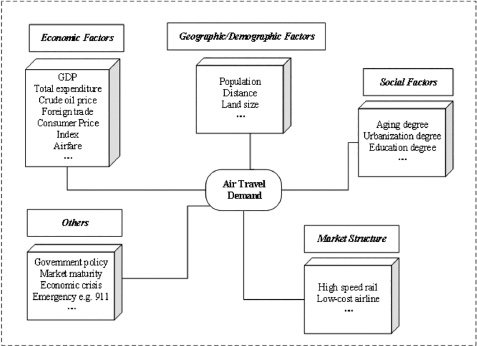
Demirsoy (2012) defined air travel demand determinants as factors which can make it possible for people to travel and increase the number of individuals’ travel. He proposed a slightly different division of air travel demand determinants, which is economic factors, geographic and demographic factors, market structure, social factors and maturity, and claimed that each group affected demand from a different perspective. Economic factors, such as GDP, expenditure, airfares and inflation, are one of the most influential drivers. Geographic and demographic factors include population, country size and urbanization level, etc. Market structure means regulated or deregulated, and the business model of airlines. And social factors represent psychological perception of the public, such as education and immigration. The final one, maturity, is a phase of the air transportation system, where the air travel demand starts to get less sensitive to income changes. Note that the maturity level within a country may differ with regard to various markets or O-D pairs. In general, determinants are the factors that not only make traveling possible but also increase traveling desire. Based on those previous studies, we summarize and reorganize the air travel demand determinants, shown in Figure 2.1.

(1) Economic factors

Air transportation and economic activity are in a close interaction. On one hand, air transportation can stimulate economic activities mainly by the enabling effect, which was defined by Ishutkina and Hansman (2008) as ‘the total economic impact on employment and income generated by the economic activities which are dependent on the availability of air transportation services’. On the other hand, economic activities can in turn generate more air transportation demand. According to Boeing Company’s report in the year 2011, air transportation revenues on average constitute 1 percent of the country’s GDP regardless of economy size, and at the regional level, about 60 to 80 percent of air travel growth can be attributed to economic growth.

Figure 2.1 Determinants of air travel demand

The most commonly discussed economic factor in the literature is income. GDP is usually taken as a proxy for income (e.g., Marazzo et al., 2010; Fernandes et al., 2010; Wang et al., 2010), while several studies chose GDP per capita instead of GDP (e.g., Cline et al., 1998; Murel and O’Connell, 2011; Demirsoy, 2012). Total expenditure, reflecting economic activities from another perspective, is also commonly used as an economic factor (e.g., Ba-fail et al., 2000; Abed et al., 2001). In addition, as a measurement of international economic activities, foreign trade has also been discussed in literature (e.g., Fildes et al., 2011). Countries whose economics are tied closely to international trade usually tend to have a higher air travel growth rate.

In addition to income and expenditure, cost is another important economic factor. Taken as a proxy variable of cost, energy price is usually assumed to have a negative influence on air travel demand. For example, Carson et al. (2011) investigated the impact of both the spot price of jet fuel and the oil futures price in detail. Consumer Price Index (CPI) is also widely used, as a proxy of airfares (e.g., Abed et al., 2001; Alperovich and Machnes, 1994). In addition, exchange rate is also a valid determinant mainly for international routes’ demand (e.g., Dargay and Hanly, 2001).

(2) Geographic and demographic factors

Population, both size and density, is the most common factor in literature among demographic factors. For example, empirical results of Abed et al. (2001) showed that a demand model with population size and total expenditure as explanatory variables performed best. Bhadra and Wells (2005) also pointed out that passenger demand was heavily influenced by the population. Similar studies include Jorge-Calderòn (1997), Grosche et al. (2007) and Kopsch (2012). In addition, several studies, e.g., Alperovich and Machnes (1994), recommended to use the ratio of passenger number to population size, to avoid problems such as multicollinearity.

Geographic factors, such as location, geographical size and distance, have been confirmed as significant determinants of air travel demand. Size of a country or region usually plays an important role. For example, Bhadra and Wells (2005) clarified that there was more air travel demand within a state with a larger size, in the case of the US domestic air transportation market. Distance is also one of the most common geographic factors, especially for city-pair demand (e.g., Jorge-Calderòn, 1997; Grosche et al., 2007). European countries generally have lower air travel demand due to the proximity of economic partners and an advanced land transportation system. In a similar way, the location of a country or region has a significant influence on air travel demand. Countries which are isolated geographically, such as New Zealand and Singapore, usually have higher air travel demand, as Ishutkina and Hansman (2008) proved.

(3) Social factors

Social factors can be defined as the facts and experiences that influence individuals’ personality, attitudes and lifestyles. Because the society is continually changing, those air passengers’ or potential passengers’ lifestyles and attitudes for air transportation may constantly change. Thus, social factors also play a vital role in air travel demand. Compared to economic factors and geographic/demographic factors, social factors are much more difficult to quantify. Psychological, environmental, immigration issues and changing lifestyles are common social factors for air travel demand (Demirsoy, 2012).

Steiner (1967) concluded that ‘travel habits or patterns are rapidly changing as young people who have grown up in an environment of safe and reliable air travel regard flying as a normal means of extending their social and educational horizons’, and he also claimed that the higher the education level, the more air travel taken by these individuals. Hence, we may assume that highly educated societies have more air travel demand, where aging degree and education degree may be considered as proxies for these factors.

The growth of the leisure air transportation market is mainly affected by these social factors. For example, Graham (2000) showed that people were taking longer and more holidays than before, which in turn stimulated the development of the air transportation market. In addition, Demirsoy (2012) thought that the strong migration trend from rural to urban, especially in emerging countries such as China, would further stimulate air travel demand, because migrants tend to travel regularly to go back to their hometowns and visit friends and relatives.

(4) Market structure

Market structure mainly represents a competition between air transportation and the land transportation system, or a competition among various business modes.

Within the land transportation system, high speed rail is the most competitive mode to air transportation in terms of speed and service quality, especially for a relative short-haul distance. For example, Kim et al. (2003) discussed the air travel demand changes of Seoul-Busan and Seoul-Daegu airlines when a competitive high speed rail was opened. Results showed that air travel demand of airlines was forecasted to decrease by 69.5 percent and 59.0 percent, respectively, due to the high speed rail’s opening. Park and Ha (2006) also analyzed the effects on air travel demand of a new high speed rail’s opening, through the stated preference survey method. And the actual results revealed that only 28 percent of air passengers still preferred to travel by air after the opening of high speed rail.

On the other hand, the introduction of new business modes usually has a significant influence on market structure and air travel demand. For example, low-cost mode is the most popular topic in the literature. Many studies have investigated the effect of low-cost mode on air travel demand (e.g., Gillen and Lall, 2004; Barrett, 2004; O’Connell and Williams, 2005). With low-cost business mode, more people are able to afford flying. For instance, low-cost airlines stimulated a major proportion of European air travel demand especially after enlargement of the European Union member states (Steiner et al., 2008). And Mason (2005) also pointed out that the introduction of low-cost mode had stimulated the development of the tourism industry.

(5) Others

Government regulation and policy are important determinants for air travel demand. For example, deregulation was a milestone of the air transportation industry in almost every country. It freed the market and increased the air travel demand extensively and unprecedentedly. Ishutkina and Hansman (2008) stated that changes in the regulatory framework such as deregulations and liberalizations might cause sudden changes in air travel demand patterns. And the industry will continuously adapt to various government policies such as the environmental regulation.

In addition, emergencies such as the outbreak of SARS and the 911 terrorist attacks may also have an effect on air travel demand, more likely in a short-term future. Studies that analyzed the impact of 911 on air travel demand include Lai and Lu (2005) and Ito and Lee (2005).

2.3 Conclusions

In this chapter, we reviewed the existing research about demand forecasting in a two-step way. Firstly, in section 2.1, we focused on the general demand and classified these studies by the forecasting time horizons, i.e., short term, medium term and long term, to review the common methods applied in different forecasting time horizons.

In short-term demand forecasting, we mainly focus on the two typical fields in demand forecasting literature to serve as the representatives, including electricity demand and tourism demand, where the definition for a short term is 1 hour to 1 week and 1 month to 12 months, respectively. For the electricity demand, regression models are conventional in the short-term electricity demand forecasting literature, due to their ability in modeling the relationships between the explained variable and its explanatory variables, such as the weather variables; while some other studies considered that the univariate models were sufficient for a short-term electricity demand forecasting because weather variables often change smoothly over a short term, and the change can also be captured by the demand series itself. For the short-term tourism demand forecasting, univariate time series models such as ARIMA models are widely used. These models pay particular attention to exploring historic data trends and patterns (e.g., seasonality) of the tourism demand series itself. Multivariate econometric models, such as VAR and VEC models, are also popular in the short-term tourism demand forecasting. The major advantage of these multivariate models is the ability to analyze the causal relationships between the tourism demand series and its influencing factors, as well as to capture the interdependence among various time series. In addition to these individual forecasting models, combination forecasting models are also widely applied in short-term forecasting literature.

In the medium-term forecasting, due to the similarity of a medium-term economic forecasting with what we have described about demand forecasting, we summarized the common methods for a medium-term economic forecasting, to provide an insight view about forecasting methods selection for a 3- to 5-year ahead demand forecasting. A medium-term economic forecasting is usually performed by government authorities and many national or international institutions, and a medium-term forecast is particularly vital for the planning of a country’s public budgets and policy recommendations. The methods for potential output estimation and medium-term economic forecasting can be generally classified into three main groups, including the univariate statistical filters, multivariate time series models and production function approaches. For the first method, the actual output time series is decomposed into trend component and cyclical component by some univariate statistical filters with some statistical criteria. Then the potential output is defined as the permanent trend component and the output gap corresponds to the transitory cyclical component. The typical methods include the HP filter. For the second method, the multivariate time series models incorporate the knowledge of economic structure and develop models to estimate the potential output and the output gap. This group of methods overcomes the limitations of univariate filters. These methods typically include a multivariate filter and the SVAR models. And the last method is called the production function approach (PFA), which considers the potential output as the level of economic output when all production factors are fully utilized. The biggest advantage of the PFA approach is to explicitly identify the sources of output growth, i.e., capital, labor, technical progress and sometimes intermediate inputs. Besides the massive discussion in academic articles, the PFA method is also popular in practice – international institutions such as the OECD, IMF and European Commission are all adopting the PFA method in their medium-term economic forecasting processes.

In the long-term demand forecasting, a long term is set as a period of longer than 5 years. Thus, the long-term demand forecasts rely greatly on researchers’ domain knowledge and the assumed future growth rates of some related variables such as economic growth, and a long-term demand forecasting model should be able to translate the changes in those variables into subsequent changes in the future demand. The long-term demand forecasting methods mainly include the scenario-based methods, the simulation-based methods, common multivariate and univariate methods and others. For the scenario-based methods, setting scenarios is a common way to express the uncertainty about the future, and the scenarios mean several optional and reasonable assumptions for the future. Common demand forecasting models, such as regression models, coupled with various scenarios have been most frequently used for long-term demand forecasting.

Secondly, in section 2.2, we focused on the air travel demand. The selection of forecasting models often depends on many aspects including the specific demand category under consideration, the forecasting time horizon, the availability of data, etc. Thus, we discussed common forecasting methods for various categories of air travel demand, and we grouped the air travel demand into three main categories according to the geographical scope, including air travel demand of O-D pairs, air travel demand of an airport and nationwide air travel demand. For the air travel demand of O-D pairs, gravity models are intuitively appropriate and also widely applied in demand forecasting literature. And the service quality-related factors are usually considered and added into the classic gravity models, to improve the forecasting performance. Other forecasting methods, such as AI-based models and econometric models, have also been applied for O-D pair air travel demand. For the air travel demand of an airport, econometric regression models considering social and economic factors are widely applied in literature. In recent years, AI-based forecasting models are particularly popular especially for modeling time series with high volatility and irregularity. Thus, some studies developed AI-based combination forecasting models for airport-specific demand. At last, for the nationwide air travel demand, linear regression models are the most popular method with the ability to quantify the impact of economic and environment factors on air travel demand, especially for medium-term and even long-term forecasting. Besides linear regression models, Holt–Winters forecasting models are also applied in several studies, based on a long time series which is assumed to demonstrate the whole historical trend.

In section 2.2, we also summarized the determinants for general air travel demand. According to our research results, the determinants can be classified into five main groups, including the economic factors (e.g., GDP, total expenditure, oil price, foreign trade, etc.), the geographic and demographic factors (e.g., population, distance and land size), the social factors (e.g., aging degree, urbanization degree and education degree), the factors about market structure (e.g., high speed rail and low-cost airline) and others such as the government policy, the market maturity and economic crises. Hence, the air travel demand is influenced by a complex factor system, which will make the demand forecasting more difficult.

To sum up, demand forecasting is always a difficult task and the selection and construction of forecasting models mainly depend on the nature of the demand category under consideration, the short-term or long-term characteristics, the required degree of forecasting accuracy and the availability of suitable historical data. Thus, better forecasting models are required both for the academic research purpose and for the management decision-making in practice.

References

Abed, S. Y., Ba-Fail, A. O., and Jasimuddin, S. M. (2001). An econometric analysis of international air travel demand in Saudi Arabia. Journal of Air Transport Management, 7(3), 143–148.
Abrahams, M. (1983). A service quality model of air travel demand: An empirical study. Transportation Research Part A: General, 17(5), 385–393.
Adams, F. G., and Shachmurove, Y. (2008). Modeling and forecasting energy consumption in China: Implications for Chinese energy demand and imports in 2020. Energy Economics, 30(3), 1263–1278.
Agarwal, V., and Talley, W. K. (1985). The demand for international air passenger service provided by US air carriers. International Journal of Transport Economics, 12(1), 63–70.
Alhumoud, J. (2008). Freshwater consumption in Kuwait: Analysis and forecasting. Journal of Water Supply Research and Technology-AQUA, 57(4), 279–288.
Almutaz, I., Ali, E., Khalid, Y., and Ajbar, A. H. (2013). A long-term forecast of water demand for a desalinated dependent city: Case of Riyadh City in Saudi Arabia. Desalination and Water Treatment, 51(31–33), 5934–5941.
Alperovich, G., and Machnes, Y. (1994). The role of wealth in the demand for international air travel. Journal of Transport Economics and Policy, 28(2), 163–173.
Al-Saba, T., and El-Amin, I. (1999). Artificial neural networks as applied to long-term demand forecasting. Artificial Intelligence in Engineering, 13(2), 189–197.
Andreoni, A., and Postorino, M. N. (2006). A Multivariate ARIMA Model to Forecast Air Transport Demand. Proceedings of the Association for European Transport and Contributors, Strasbourg, France.
Ardakani, F. J., and Ardehali, M. M. (2014). Novel effects of demand side management data on accuracy of electrical energy consumption modeling and long-term forecasting. Energy Conversion and Management, 78, 745–752.
Armstrong, J. S. (Ed.). (2001). Principles of Forecasting: A Handbook for Researchers and Practitioners. New York, Springer Science & Business Media.
Azari, A., Shariaty-Niassar, M., and Alborzi, M. (2012). Short-term and medium-term gas demand load forecasting by neural networks. Iranian Journal of Chemistry and Chemical Engineering, 31(4), 77–84.
Babel, M. S., Maporn, N., and Shinde, V. R. (2014). Incorporating future climatic and socioeconomic variables in water demand forecasting: A case study in Bangkok. Water Resources Management, 28(7), 2049–2062.
Ba-fail, A. O., Abed, S. Y., Jasimuddin, S. M., and Jeddah, S. A. (2000). The determinants of domestic air travel demand in the Kingdom of Saudi Arabia. Journal of Air Transportation World Wide, 5(2), 72–86.
Barrett, S. D. (2004). How do the demands for airport services differ between full-service carriers and low-cost carriers? Journal of Air Transport Management, 10(1), 33–39.
Beffy, P. O., Ollivaud, P., Richardson, P., and Sédillot, F. (2006). New OECD Methods for Supply-Side and Medium-Term Assessments (No. 482). OECD Economics Department.
Bermúdez, J. D., Segura, J. V., and Vercher, E. (2007). Holt–Winters forecasting: An alternative formulation applied to UK air passenger data. Journal of Applied Statistics, 34(9), 1075–1090.
Bhadra, D., and Kee, J. (2008). Structure and dynamics of the core US air travel markets: A basic empirical analysis of domestic passenger demand. Journal of Air Transport Management, 14(1), 27–39.
Bhadra, D., and Wells, M. (2005). Air travel by state: Its determinants and contributions in the United States. Public Works Management & Policy, 10(2), 119–137.
Burger, C. J. S. C., Dohnal, M., Kathrada, M., and Law, R. (2001). A practitioner’s guide to time-series methods for tourism demand forecasting – a case study of Durban, South Africa. Tourism Management, 22(4), 403–409.
Cancelo, J. R., Espasa, A., and Grafe, R. (2008). Forecasting the electricity load from one day to one week ahead for the Spanish system operator. International Journal of Forecasting, 24(4), 588–602.
Cao, Z., Yuan, P., and Ma, Y. B. (2014). Energy demand forecasting based on economy-related factors in China. Energy Sources, Part B: Economics, Planning, and Policy, 9(2), 214–219.
Carnot, N., Koen, V., and Tissot, B. (2005). Economic Forecasting. New York, Palgrave Macmillan.
Carson, R. T., Cenesizoglu, T., and Parker, R. (2011). Forecasting (aggregate) demand for US commercial air travel. International Journal of Forecasting, 27(3), 923–941.
Castelli, L., Pesenti, R., and Ukovich, W. (2003). An Airline-Based Multilevel Analysis of Airfare Elasticity for Passenger Demand. Proceeding of the 7th Air Transport Research Society Conference, Toulouse, France.
Chai, J., Wang, S., Wang, S., and Guo, J. E. (2012). Demand forecast of petroleum product consumption in the Chinese transportation industry. Energies, 5(3), 577–598.
Charytoniuk, W., Chen, M. S., and Van Olinda, P. (1998). Non-parametric regression based short-term load forecasting. IEEE Transactions on Power Systems, 13(3), 725–730.
Chen, K. Y., and Wang, C. H. (2007). Support vector regression with genetic algorithms in forecasting tourism demand. Tourism Management, 28(1), 215–226.
Chen, T. (2012). Forecasting the long-term electricity demand in Taiwan with a Hybrid FLR and BPN approach. International Journal of Fuzzy Systems, 14(3), 361–371.
Cho, V. (2001). Tourism forecasting and its relationship with leading economic indicators. Journal of Hospitality and Tourism Research, 25(4), 399–420.
Cho, V. (2003). A comparison of three different approaches to tourist arrival forecasting. Tourism Management, 24(3), 323–330.
Claus, I. (2003). Estimating potential output for New Zealand. Applied Economics, 35(7), 751–760.
Cline, R. C., Ruhl, T. A., Gosling, G. D., and Gillen, D. W. (1998). Air transportation demand forecasts in emerging market economies: A case study of the Kyrgyz Republic in the former Soviet Union. Journal of Air Transport Management, 4(1), 11–23.
Cotis, J. P., Elmeskov, J., and Mourougane, A. (2004). Estimates of potential output: benefits and pitfalls from a policy perspective. The euro area business cycle: stylized facts and measurement issues. Centre for Economic Policy Research, 35–60.
Dargay, J., and Hanly, M. (2001). The Determinants of the Demand for International Air Travel to and from the UK. Proceedings of the 9th World Conference on Transport Research, Edinburgh, Scotland.
De Felice, M., Alessandri, A., and Catalano, F. (2015). Seasonal climate forecasts for medium-term electricity demand forecasting. Applied Energy, 137, 435–444.
Demirsoy, C. (2012). Analysis of Stimulated Domestic Air Transport Demand in Turkey. Erasmus University Thesis Repository, Rotterdam, The Netherlands.
Ediger, V. Ş., and Akar, S. (2007). ARIMA forecasting of primary energy demand by fuel in Turkey. Energy Policy, 35(3), 1701–1708.
Fabiani, S., and Mestre, R. (2004). A system approach for measuring the euro area NAIRU. Empirical Economics, 29(2), 311–341.
Fernandes, E., and Pacheco, R. R. (2010). The causal relationship between GDP and domestic air passenger traffic in Brazil. Transportation Planning and Technology, 33(7), 569–581.
Fildes, R., Wei, Y., and Ismail, S. (2011). Evaluating the forecasting performance of econometric models of air passenger traffic flows using multiple error measures. International Journal of Forecasting, 27(3), 902–922.
Fouré, J., Bénassy-Quéré, A., and Fontagné, L. (2012). The Great Shift: Macroeconomic Projections for the World Economy at the 2050 Horizon (No.2012–3). Social Science Research Network.
Fridström, L., and Thune-Larsen, H. (1989). An econometric air travel demand model for the entire conventional domestic network: The case of Norway. Transportation Research Part B: Methodological, 23(3), 213–223.
Gerlach, S., and Smets, F. (1999). Output gaps and monetary policy in the EMU area. European Economic Review, 43(4), 801–812.
Ghobrial, A., and Kanafani, A. (1995). Quality-of-service model of intercity air-travel demand. Journal of Transportation Engineering, 121(2), 135–140.
Gil-Alana, L. A. (2005). Modelling international monthly arrivals using seasonal univariate long-memory processes. Tourism Management, 26(6), 867–878.
Gil-Alana, L. A., Gracia, F. P. D., and Cunado, J. (2004). Seasonal fractional integration in the Spanish tourism quarterly time-series. Journal of Travel Research, 42(4), 408–414.
Gillen, D., and Lall, A. (2004). Competitive advantage of low-cost carriers: Some implications for airports. Journal of Air Transport Management, 10(1), 41–50.
Goh, C., and Law, R. (2002). Modeling and forecasting tourism demand for arrivals with stochastic non-stationary seasonality and intervention. Tourism Management, 23(5), 499–510.
Graham, A. (2000). Demand for leisure air travel and limits to growth. Journal of Air Transport Management, 6(2), 109–118.
Grant, J., Eltoukhy, M., and Asfour, S. (2014). Short-term electrical peak demand forecasting in a large government building using artificial neural networks. Energies, 7(4), 1935–1953.
Grosche, T., Rothlauf, F., and Heinzl, A. (2007). Gravity models for airline passenger volume estimation. Journal of Air Transport Management, 13(4), 175–183.
Gross, G., and Galiana, F. D. (1987). Short-term load forecasting. Proceedings of the IEEE, 75(12), 1558–1573.
Grubb, H., and Mason, A. (2001). Long lead-time forecasting of UK air passengers by Holt-Winters methods with damped trend. International Journal of Forecasting, 17(1), 71–82.
Haida, T., and Muto, S. (1994). Regression based peak load forecasting using a transformation technique. IEEE Transactions on Power Systems, 9(4), 1788–1794.
Hernández, L., Baladrón, C., Aguiar, J. M., Calavia, L., Carro, B., Sánchez-Esguevillas, A., and Lloret, J. (2013). Experimental analysis of the input variables’ relevance to forecast next day’s aggregated electric demand using neural networks. Energies, 6(6), 2927–2948.
Ho, K. L., Hsu, Y. Y., Chen, C. F., Lee, T. E., Liang, C. C., Lai, T. S., and Chen, K. K. (1990). Short term load forecasting of Taiwan power system using a knowledge-based expert system. IEEE Transactions on Power Systems, 5(4), 1214–1221.
Hodrick, R. J., and Prescott, E. C. (1997). Postwar US business cycles: An empirical investigation. Journal of Money, Credit, and Banking, 29(1), 1–16.
Hor, C. L., Watson, S. J., and Majithia, S. (2005). Analyzing the impact of weather variables on monthly electricity demand. IEEE Transactions on Power Systems, 20(4), 2078–2085.
Hostland, D., and Côté, D. (1993). Measuring Potential Output and the NAIRU as Unobserved Variables in a Systems Framework. Ottawa, Bank of Canada.
Huarng, K. H., Yu, T. H. K., and Sole Parellada, F. (2011). An innovative regime switching model to forecast Taiwan tourism demand. The Service Industries Journal, 31(10), 1603–1612.
Ishutkina, M. A., and Hansman, R. J. (2008). Analysis of Interaction Between Air Transportation and Economic Activity. Proceedings of the 26th Congress of Internationals Council of the Aeronautical Sciences, Anchorage, Alaska.
Ito, H., and Lee, D. (2005). Assessing the impact of the September 11 terrorist attacks on US airline demand. Journal of Economics and Business, 57(1), 75–95.
Jorge-Calderón, J. D. (1997). A demand model for scheduled airline services on international European routes. Journal of Air Transport Management, 3(1), 23–35.
Kappler, M. (2007). Projecting the Medium-Term: Outcomes and Errors for GDP Growth. ZEW-Centre for European Economic Research Discussion Paper, No. 07–068.
Karlaftis, M. G., Zografos, K. G., Papastavrou, J. D., and Charnes, J. M. (1996). Methodological framework for air-travel demand forecasting. Journal of Transportation Engineering, 122(2), 96–104.
Kim, K. W., Seo, H. Y., and Kim, Y. (2003). Forecast of domestic air travel demand change by opening the high speed rail. KSCE Journal of Civil Engineering, 7(5), 603–609.
Koen, R., and Holloway, J. (2014). Application of multiple regression analysis to forecasting South Africa’s electricity demand. Journal of Energy in Southern Africa, 25(4), 48–58.
Kon, S. C., and Turner, L. W. (2005). Neural network forecasting of tourism demand. Tourism Economics, 11(3), 301–328.
Kopsch, F. (2012). A demand model for domestic air travel in Sweden. Journal of Air Transport Management, 20, 46–48.
Kulendran, N., and Wilson, K. (2000). Is there a relationship between international trade and international travel? Applied Economics, 32(8), 1001–1009.
Kuttner, K. N. (1994). Estimating potential output as a latent variable. Journal of Business & Economic Statistics, 12(3), 361–368.
Lai, S. L., and Lu, W. L. (2005). Impact analysis of September 11 on air travel demand in the USA. Journal of Air Transport Management, 11(6), 455–458.
Laxton, D., and Tetlow, R. (1992). A Simple Multivariate Filter for the Measurement of Potential Output (No. 59). Ottawa, Bank of Canada.
Li, T., and Trani, A. A. (2014). A model to forecast airport-level general Aviation demand. Journal of Air Transport Management, 40, 192–206.
Liang, Y. H. (2014). Forecasting models for Taiwanese tourism demand after allowance for Mainland China tourists visiting Taiwan. Computers & Industrial Engineering, 74, 111–119.
Lim, C., and McAleer, M. (2001). Cointegration analysis of quarterly tourism demand by Hong Kong and Singapore for Australia. Applied Economics, 33(12), 1599–1619.
Mallikarjuna, C., and Raghu Kanth, S. T. G. (2010). Forecasting the air traffic for north-east Indian cities. Advances in Adaptive Data Analysis, 2(1), 81–96.
Marazzo, M., Scherre, R., and Fernandes, E. (2010). Air transport demand and economic growth in Brazil: A time series analysis. Transportation Research Part E: Logistics and Transportation Review, 46(2), 261–269.
Mason, K. J. (2005). Observations of fundamental changes in the demand for aviation services. Journal of Air Transport Management, 11(1), 19–25.
McMorrow, K., and Roeger, W. (2001). Potential Production: Measurement Methods, New Economy Influences and Scenarios for 2001–10. European Economy Economic Papers, No.150.
McNown, R., Aburizaizah, O. S., Howe, C., and Adkins, N. (2015). Forecasting annual water demands dominated by seasonal variations: The case of water demands in Mecca. Applied Economics, 47(6), 544–552.
Mirasgedis, S., Sarafidis, Y., Georgopoulou, E., Lalas, D. P., Moschovits, M., Karagiannis, F., and Papakonstantinou, D. (2006). Models for mid-term electricity demand forecasting incorporating weather influences. Energy, 31(2), 208–227.
Murel, M., and O’Connell, J. F. (2011). Potential for Abu Dhabi, Doha and Dubai airports to reach their traffic objectives. Research in Transportation Business & Management, 1(1), 36–46.
O’Connell, J. F., and Williams, G. (2005). Passengers’ perceptions of low cost airlines and full service carriers: A case study involving Ryanair, Aer Lingus, Air Asia and Malaysia Airlines. Journal of Air Transport Management, 11(4), 259–272.
Öğünç, F., and Ece, D. (2004). Estimating the output gap for Turkey: An unobserved components approach. Applied Economics Letters, 11(3), 177–182.
Oh, C. O., and Morzuch, B. J. (2005). Evaluating time-series models to forecast the demand for tourism in Singapore: Comparing within sample and post-sample results. Journal of Travel Research, 43(4), 404–413.
Özgen, C. (2011). Air passenger demand forecasting for planned airports, case study: Zafer and Or-gi airports in Turkey. Middle East Technical University Thesis Repository, Ankara, Turkey.
Park, Y., and Ha, H. K. (2006). Analysis of the impact of high-speed railroad service on air transport demand. Transportation Research Part E: Logistics and Transportation Review, 42(2), 95–104.
Pourazarm, E., and Cooray, A. (2013). Estimating and forecasting residential electricity demand in Iran. Economic Modelling, 35, 546–558.
Pukšec, T., Krajačić, G., Lulić, Z., Mathiesen, B. V., and Duić, N. (2013). Forecasting long-term energy demand of Croatian transport sector. Energy, 57, 169–176.
Rahman, S., and Hazim, O. (1996). Load forecasting for multiple sites: Development of an expert system-based technique. Electric Power Systems Research, 39(3), 161–169.
Samagaio, A., and Wolters, M. (2010). Comparative analysis of government forecasts for the Lisbon airport. Journal of Air Transport Management, 16(4), 213–217.
Scacciavillani, F., and Swagel, P. (2002). Measures of potential output: An application to Israel. Applied Economics, 34(8), 945–957.
Shan, J., and Wilson, K. (2001). Causality between trade and tourism: Empirical evidence from China. Applied Economics Letters, 8(4), 279–283.
Soares, L. J., and Medeiros, M. C. (2008). Modeling and forecasting short-term electricity load: A comparison of methods with an application to Brazilian data. International Journal of Forecasting, 24(4), 630–644.
Song, H., and Li, G. (2008). Tourism demand modelling and forecasting – a review of recent research. Tourism Management, 29(2), 203–220.
Song, H., and Witt, S. F. (2006). Forecasting international tourist flows to Macau. Tourism Management, 27(2), 214–224.
Steiner, J. E. (1967). Aircraft evolution and airline growth. Financial Analysts Journal, 23(2), 85–92.
Steiner, S., Božičević, A., and Mihetec, T. (2008). Determinants of European air traffic development. Transport Problems, International Scientific Journal, 3(4), 73–84.
Strand, S. (1999). Airport-specific traffic forecasts: the resultant of local and non-local forces. Journal of Transport Geography, 7(1), 17–29.
Taylor, J. W. (2003). Short-term electricity demand forecasting using double seasonal exponential smoothing. Journal of the Operational Research Society, 54(8), 799–805.
Taylor, J. W. (2008). An evaluation of methods for very short-term load forecasting using minute-by-minute British data. International Journal of Forecasting, 24(4), 645–658.
Taylor, J. W. (2010). Triple seasonal methods for short-term electricity demand forecasting. European Journal of Operational Research, 204(1), 139–152.
Taylor, J. W., De Menezes, L. M., and McSharry, P. E. (2006). A comparison of univariate methods for forecasting electricity demand up to a day ahead. International Journal of Forecasting, 22(1), 1–16.
Taylor, J. W., and McSharry, P. E. (2007). Short-term load forecasting methods: An evaluation based on European data. IEEE Transactions on Power Systems, 22(4), 2213–2219.
Teyssier, N. (2012). How the Consumer Confidence Index Could Increase Air Travel Demand Forecast Accuracy? Cranfield University Thesis Repository, Cranfield.
Turner, L. W., and Witt, S. F. (2001). Factors influencing demand for international tourism: Tourism demand analysis using structural equation modelling, revisited. Tourism Economics, 7(1), 21–38.
Uddin, W., McCullough, B. F., and Crawford, M. M. (1985). Methodology for Forecasting Air Travel and Airport Expansion Needs. Proceedings of 64th Annual Meeting of the Transportation Research Board, Washington DC.
Wang, S. J., Sui, D., and Hu, B. (2010). Forecasting technology of national-wide civil aviation traffic. Journal of Transportation Systems Engineering and Information Technology, 10(6), 95–102.
Wei, W., and Hansen, M. (2006). An aggregate demand model for air passenger traffic in the hub-and-spoke network. Transportation Research Part A: Policy and Practice, 40(10), 841–851.
Xiao, Y., Liu, J. J., Hu, Y., Wang, Y., Lai, K. K., and Wang, S. (2014). A neuro-fuzzy combination model based on singular spectrum analysis for air transport demand forecasting. Journal of Air Transport Management, 39, 1–11.
Xie, G., Wang, S., and Lai, K. K. (2014). Air Passenger Forecasting by Using a Hybrid Seasonal Decomposition and Least Squares Support Vector Regression Approach. DOI: http://2013.isiproceedings.org/Files/CPS205-P37-S.pdf
Yang, H. H., Chen, S. H., Hung, J. Y., Hung, C. T., and Chung, M. L. (2010). Utilization of Genetic Programming to Establish Demand Forecast in Taiwan International Flights. Proceedings of 2nd International Conference on Information Engineering and Computer Science, Wuhan, China.
Zjavka, L. (2015). Short-term power demand forecasting using the differential polynomial neural network. International Journal of Computational Intelligence Systems, 8(2), 297–306.