3   Theoretical basis – TEI@I methodology

According to previous chapters’ discussion, air travel demand forecasting is a vital but tough task. On one hand, traditional statistical models that only rely on historical data are insufficient for achieving a satisfactory forecasting performance. On the other hand, expert knowledge plays an increasingly important role in the demand forecasting, especially for a medium-term and long-term future. Hence, a forecasting approach combining traditional mathematical models with expert knowledge for various forecasting time horizons is urgently needed.

In this chapter, we will introduce a system analysis methodology named TEI@I methodology, as our theoretical basis in this book to guide our air travel demand forecasting model constructions and selections. Section 3.1 introduces the TEI@I methodology from a theoretical point of view; section 3.2 firstly constructs a general forecasting framework based on TEI@I methodology, and describes the main function modules in this forecasting framework. Then based on the constructed forecasting framework, we generate an air travel demand forecasting framework for this book; section 3.3 introduces common forecasting models and methods which can be chosen and incorporated in the TEI@I methodology; section 3.4 concludes this chapter.

3.1 Introduction

In the analysis and research of a system, the complex interaction between various internal components and external factors results in a complex system with burstiness, volatility, nonlinearity and uncertainty. Hence, the traditional analysis methods cannot meet the needs of analyzing such a complex system. The difficulty in forecasting a complex system, due to its inherent complexity and nonlinearity, has already attracted much attention of academic researchers and business practitioners. Various forecasting methods have been constructed to solve these forecasting problems. However, to analyze the complex system in a better way, some new methodology must be created. Based on this research background and motivation, Wang (2004) proposed the new concept of TEI@I methodology.

Proposed by Wang (2004), TEI@I is a system analysis methodology proposed for handling complex systems at first. In fact, the TEI@I methodology is a brand new methodology that combines the traditional statistical techniques and the emerging artificial intelligence techniques. As the name hints, TEI@I methodology is a systematic integration (@) of text mining (T), econometrics (E) and intelligence (I) techniques. In this creative methodology, it systematically integrates the text mining techniques, econometrical models, artificial intelligence techniques and integration techniques. TEI@I methodology essentially reflects the ‘disintegrating, then integrating’ idea. Firstly, the complex system is decomposed into several components, and the econometrical models are constructed for modeling the main trend component in the original system, while the artificial techniques are used for analyzing the nonlinearity and uncertainty in the original system. Secondly, the text mining techniques are applied in mining the complex system’s burstiness and volatility. Finally, based on the integration idea, we integrate all individual parts into a final analysis result, as the final analysis for the original complex system.

In the previous academic articles, TEI@I methodology was especially applied to analyze and forecast the complicated, nonlinear, unstable and uncertain systems, such as oil price forecasting (e.g., Wang et al., 2005; Yu et al., 2008), exchange rate forecasting (e.g., Wang et al., 2007), housing price forecasting (e.g., Yan et al., 2007) and port logistics forecasting (e.g., Tian et al., 2009).

3.2 TEI@I methodology for air travel demand forecasting

In this section, a general description of the TEI@I methodology is presented. Firstly, we describe a general forecasting framework of the TEI@I methodology, and then discuss some main components of the TEI@I methodology: man-machine interface module, web-based text mining module, rule-based expert system module, ARIMA-based econometrical linear forecasting module, ANN-based nonlinear forecasting module and bases and bases management module. Within the TEI@I methodology forecasting framework, we then propose a novel nonlinear integrated air travel demand forecasting framework.

3.2.1 A general framework of TEI@I methodology

Based on the integration idea, TEI@I methodology integrates the various techniques, such as the text mining techniques, econometrical models and artificial intelligence techniques, to provide integrated analysis results. The basic structure of the TEI@I methodology when applied in demand forecasting modeling is shown in Figure 3.1.

As Figure 3.1 shows, the framework of TEI@I methodology consists of six main function modules, i.e., the man-machine interface module, web-based text mining module, rule-based expert system module, ARIMA-based econometrical linear forecasting module, ANN-based nonlinear forecasting module, and bases and bases management module. The functions and internal mechanisms of each module are introduced in detail as follows.

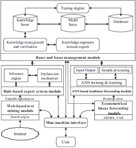
(1) Man-machine interface module

The man-machine interface (MMI) module is a graphical window through which the users can provide, get and exchange information within the TEI@I methodology framework. In detail, it handles all inputs and outputs between users and the TEI@I system of all six modules. It also handles all communications with the knowledge engineers or domain experts during the development of the bases and bases management module. In the same way, it can interact with the other four main modules: the econometrical linear forecasting module via the ARIMA models, VAR models, etc., rule-based expert system module via the inference engine and explanation mechanism, web-based text mining module via the search engine and ANN-based error correction module. In some sense, it can be considered to be an open platform communicating with users and interacting with other components of the TEI@I methodology.

(2) Web-based text mining module

The web-based text mining (WTM) module is a major component of the TEI@I methodology. The complex systems are usually unstable markets with high volatility, and are often affected by many related factors with unstructured historical information. In order to improve the forecasting accuracy, these related factors must be taken into consideration. Therefore, it is necessary to collect related information from the Internet and analyze its effects on the system. However, it is very difficult to collect the related knowledge from the Internet. With the advancement of computational techniques, WTM (e.g., Shi, 2002; Rajman and Besancon, 1998) is believed to be one of the most effective techniques of collecting this type of information. In this forecasting framework, the main goal of the WTM module is to collect related information affecting the variability of the aimed system from the Internet and to provide the collected useful information for the rule-based expert system forecasting module.

The main process of the WTM module is presented in Figure 3.2.

As shown in Figure 3.2, the whole processes of the WTM module can be divided into three phases or six processing procedures, i.e., word/phrase division processing, feature extraction processing, text structure analysis processing, text abstract generation processing, text categorization processing and text clustering processing. The three phases can be described as follows.

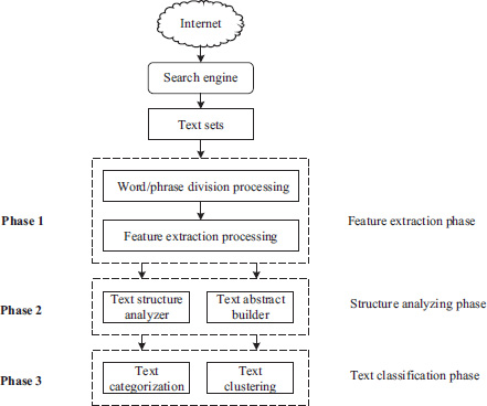
Phase 1: feature extraction phase

The Internet contains an enormous, hetero-structural and widely distributed information base in which the amount of information increases in a geometric series. In the information base, text sets that satisfy some conditions can be obtained by using a search engine. However, the collected text sets are mainly represented by web pages, which are tagged by hypertext markup language (HTML). Thus collected documents or texts are mostly semi- or non-structural information. Our task is to extract certain features that represent the text contents from these collected texts for further analysis and application. The Vector Space Model (VSM) (Salton et al., 1975) is usually introduced to analyze the text content.

Phase 2: structure analyzing phase

In the structure analyzing phase, based on the results of the text structure analyzer, text abstracts can be generated using a text abstract builder. In the text sets, web texts contain both pure texts and all kinds of hyperlinks that reflect relationships in different web pages. It is therefore necessary to analyze the text structure. By analyzing the linkage of web texts, we can judge relationships in different documents. This is useful in finding new knowledge. In the same way, by analyzing the web linkage and the number of hyperlinks, we can obtain similar and interconnected materials in different web texts, thus further increasing the efficiency of information retrieval.

Text abstracts can be generated by analyzing text structure. Text abstracts are very important in text mining because they are useful in our understanding of the whole document. There are some thematic sentences that can reflect a paper’s core ideas; and these sentences are usually located at the beginning or the end of a paper or a paragraph. The weights of these thematic sentences should therefore be larger than those of other sentences when constructing the weight function for a sentence. An automatic generation algorithm for text abstracts is presented here using PROLOG language.

Assume that T are text sets; S is the set of sentences, where S = {s₁, s₂, … , s_n} ; W_i is the weight of the ith sentence; LEN is the length of the abstract, where the initial value of LEN is usually equal to zero; LA is the length condition of the text abstract; and ABSTRACT is a list of text abstracts. The basic idea of the automatic generation algorithm for text abstracts is shown in Table 3.1.

Table 3.1 The basic idea of the text abstract generation algorithm

Create (ABSTRACT, [Wi|W], LEN)

Gets (S, Wi,TEMP), length (TEMP, L),

LEN + L <LA, !, LEN1 = LEN + L,

Append (ABSTRACT, [TEMP], ABSTRACT1),

Create (ABSTRACT1, W, LEN1).

Phase 3: text classification phase

Classification is one of the most important tasks in the data mining (Salton et al., 1975). The main goal of a classification process is to make the retrieval or query speed faster and make the retrieval more efficient and more precise than before. Here a VSM-based text categorization algorithm is introduced in detail. The core idea of the categorization algorithm is to judge the category of the testing text by calculating the similarity of eigenvectors of text features. The algorithm’s basic process can be divided into two stages.

The first stage is the sample training and learning stage. In this stage, a basic text categorization set C = {c₁, c₂, … , c_m} and its eigenvectors V(c_i) are given as targets in advance. In order to verify the algorithm’s classification capability, some training text sets S = {s₁, s₂, … , s_r} and their eigenvectors V(s_i) are chosen. By calculating the similarity of texts, we can classify the category of training texts. Here the similarity is calculated as

$Si{m}_{ik}=\frac{V_{si}\ast V_{ck}}{\left|V_{si}\right|\ast \left|V_{ck}\right|},1\le i\le r,1\le k\le m,$

(3.1)

where Sim_ik denotes the similarity between the ith category and the kth category, and V_si and V_ck represent the eigenvectors of the basic text category and training text category.

The second stage is the testing sample-identifying stage. Here we present some testing text sets T = {t₁, t₂, … , t_m} that are to be classified. We use a similarity matrix to tackle testing text sets. That is,

$similaritymatrix=[\begin{array}{l}{V}_{t1}\\ V_{t2}\\ ⋮\\ V_{tn}\end{array}]\oplus [V_{c1}{V}_{c2}\cdots V_{cm}]\text{=}\left[\begin{array}{l}Si{m}_{11}Si{m}_{12}\cdots Si{m}_{1m}\\ Si{m}_{21}Si{m}_{22}\cdots Si{m}_{2m}\\ ⋮⋮Si{m}_{ij}⋮\\ Si{m}_{n1}Si{m}_{n2}\cdots Si{m}_{nm}\end{array}\right],$

(3.2)

where

In the similarity matrix, the minimal value of every row can be obtained by a minimum function $MinSi{m}_i=\underset{j=1}{\overset{m}{\min }}\left(Si{m}_{ij}\right)$ , and then we can judge whether t_iis the most similar with c_i. Hence, text t_i will be categorized into the class of c_i.

In a similar way, we can also utilize a clustering algorithm to realize the classification. Typical algorithms include the K-means algorithm (MacQueen, 1967) and the hierarchical clustering algorithm (Olson, 1995). In this study, the VSM-based text categorization algorithm is used.

We can therefore obtain information of the influencing factors using the WTM module. In the following process, the retrieved information is sent to the rule-based expert system module.

(3) Rule-based expert system module

The key component to an expert system is the construction of the knowledge base (KB) (Yu et al., 2003). The KB is usually represented by all types of rules from knowledge engineers who collect and summarize related knowledge and information from history and from domain experts. The main function of a rule-based expert system (RES) module is to collect and extract the rules or knowledge category from the KB. Our expert system module is required to extract some rules to judge abnormal variability in the aimed complex systems by summarizing and concluding relationships between the dependent variable’s fluctuation and irregular key influencing factors that affect the dependent variable’s volatility.

To formulate a useful demand volatility mechanism for predicting the trend and movements of the future demand, researchers have to firstly observe historical demand patterns that occur frequently in the historical time series. Note that in this book, the terms ‘patterns’, ‘factors’ and ‘events’ will be used interchangeably. Secondly, the relationships between the dependent variable’s variability and the influencing factors are examined. Finally, if there are strong connections between those influencing factors and the dependent variable’s movements, then the factors are elicited from the historical data patterns examined and a KB for predicting the dependent variable’s variability can be constructed. As previously mentioned, the events such as wars, revolutions and embargoes can have an immediate impact on the movement of a demand time series. Furthermore, these factors can exert either an individual or a composite effect.

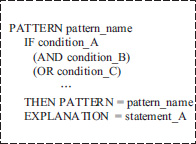
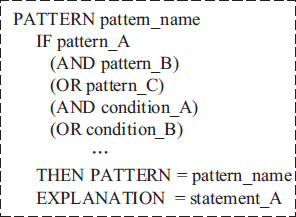
In order to represent the irregular patterns in a more organized and systematic way, the data patterns are classified into the individual patterns and the combination patterns; while compared with the combination patterns, the individual patterns have relatively simpler conditions and attributes. In this book, a pattern itself can be considered to be the representation of a rule because the conditions of a pattern can be seen as the conditions of a rule in the rule representation. Figure 3.3 and Figure 3.4 show how the individual patterns and the combination patterns are defined and constructed. The syntax of an individual pattern uses reserved words such as PATTERN, IF, AND, OR and EXPLANATION, as illustrated in Figure 3.3. If certain important events are matched with the IF condition of a particular pattern, then the pattern is identified by the conditions, and the EXPLANATION part gives the information about what the pattern really means. The individual pattern itself has its own meaning and can be an important clue in predicting the dependent variable’s volatility. Likewise, the combination patterns integrate several conditions or patterns to explain a certain sophisticated phenomenon, as illustrated in Figure 3.4.

In addition, in the RES module, the inference engine (IE) and explanation mechanism (EM) are presented to interact with users via the MMI module. The function of the IE and the EM is to provide automatic criteria comparison and interpretation of rules.

The impact of irregular events is explored and measured as the judgments of synergetic forecasts by using WTM and RES techniques. The effects will be a part of integrated forecasts as a form of judgmental adjustment.

(4) ARIMA-based econometrical linear forecasting module

The econometrical models are widely used in the time series forecasting in terms of the regression techniques. Econometrics includes a large number of modeling techniques and models, such as the Autoregressive Integrated Moving Average (ARIMA) model, vector autoregression (VAR) model and generalized moment method. If a time series is complicated, it can be divided into two parts, i.e., a linear component and a nonlinear component, by way of the decomposition techniques (e.g., Fourier decomposition and wavelet decomposition). To sum up, this econometrical module is used to model the linear components of the time series (i.e., the main trend of time series) in terms of the decomposition idea.

An Autoregressive Moving Average (ARMA) model, a typical econometrical model, is widely used. In an ARMA model, the future value of a variable is assumed to be a linear function of several lags of the explained variable and a random error. That is, the underlying process that generates the time series has the form

$\varphi \left(B\right)y_t=\theta \left(B\right)e_t$

(3.3)

where y_t and e_t are the actual value and random error at time t, respectively; B denotes the backward shift operator, i.e., $B{y}_t=y_{t-1}$ , $B^2{y}_t=y_{t-2}$ and so on; $\varphi \left(B\right)=1-{\varphi }_{1}B-\cdots -{\varphi }_p{B}^p$ , $\theta \left(B\right)=1-{\theta }_{1}B-\cdots {\theta }_q{B}^q$ , where p,q are integers and often referred to as orders of the model. The random errors, $e_t$ , are assumed to be independently and identically distributed with a mean of zero and a constant variance of ${\sigma }^2$ , i.e., $e_t\sim IID\left(0,{\sigma }^2\right)$ . If the d th difference of {y_t} is an ARMA process of order p and q, then y_t is called an ARIMA (p,d,q) process, as in Eq. (3.4):

$\varphi \left(B\right){\nabla }^d{y}_t=\theta \left(B\right)e_t$

(3.4)

Eq. (3.3) covers several important special cases of the ARIMA family of models. If θ(B)=1 or q=0, then Eq. (3.3) becomes an autoregressive (AR) model of order p, i.e., the AR(p) model. When ϕ(B)=1 or p=0, the model reduces to a moving average (MA) model of order q, i.e., the MA(q) model. One central task of the ARMA model building is to determine the appropriate model order (p,q).

Based on the earlier work of Box and Jenkins (1970), the ARIMA model involves the following five-step iterative cycle:

1. (a) Stationary test of time series, such as unit root testing;
2. (b) Identification of the ARIMA (p,d,q) structure;
3. (c) Estimation of the unknown parameters;
4. (d) Goodness-of-fit tests on the estimated residuals; and
5. (e) Forecast future outcomes based on the known data.

This five-step model building process is typically repeated several times until a satisfactory model is finally selected. The final model can then be used for the prediction purposes.

The merits of ARIMA models are two-fold. Firstly, the ARIMA models are a class of typical linear models which are designed for linear time series modeling and which can effectively capture the time series’ linear characteristics and patterns. Secondly, the theoretical foundation of ARIMA models is perfect. ARIMA models are therefore widely used in many practical applications including air travel demand forecasting. The disadvantage of the ARIMA models is that they cannot capture nonlinear patterns of the complex time series (e.g., financial time series) if the nonlinearity exists.

(5) ANN-based nonlinear forecasting module

As mentioned previously, complex time series can be decomposed into the linear and the nonlinear components. Linear components can be modeled by using the ARIMA-based econometrical linear forecasting models, but the problem is that the ARIMA models do not perform well in modeling the nonlinear components in most situations. It is therefore necessary to find an appropriate nonlinear modeling technique to fit the nonlinear components of the original time series. In this framework in Figure 3.1, artificial neural networks (ANNs) are used as the nonlinear modeling technique. ANN models with hidden layers are a class of general function approximations capable of modeling nonlinearity (Tang and Fishwick, 1993), which can capture nonlinear patterns in time series.

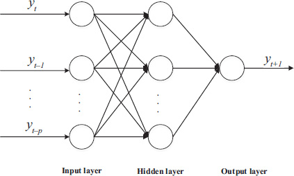
Over the past decade, ANN models have gained popularity as an emerging and excellent computational technology and they offer a new avenue to explore the dynamics and complexity of a variety of practical applications. In this section, we take the three-layer back-propagation neural network (BPNN) as an example for detailed description (see Figure 3.5) (e.g., Rumelhart et al., 1985). And we usually incorporate the Levenberg–Marquardt algorithm for a training process in the application part. Since these networks contain many interacting nonlinear neurons in the multiple layers, the networks can capture relatively complex relationships and phenomena. For a univariate time series forecasting problem, the networks’ inputs are the past lagged observations of the data series and the outputs are the future forecasted values. Each input vector has a moving window of fixed length along the sample datasets, as presented in Figure 3.5.

The BPNN models are widely used in demand forecasting literature and usually produce a successful learning and generalization result in various research areas. Detailed descriptions of the algorithm can be found in various sources (see, e.g., Kodogiannis and Lolis, 2002; Chiu et al., 1997; Yu et al., 2003).

The major merit of ANN models is their flexible nonlinear modeling capability. They can capture the nonlinear characteristics of time series very well. However, using an ANN to model linear problems may produce mixed results (e.g., Denton, 1995; Markham and Rakes, 1998). Therefore, it is not wise to blindly use the ANN models to fit any type of time series.

(6) Bases and bases management module

The bases and bases management module is an important part of the TEI@I methodology framework because the other modules all have a strong connection with this module. For example, the econometrical linear forecasting module and ANN-based error correction module will utilize the model bases (MBs) and databases (DBs), while the rule-based expert system module mainly uses the knowledge bases (KBs) and databases (DBs), as illustrated in Figure 3.1.

In the bases and bases management module, the KB is the aggregation of domain materials and rules from knowledge engineers and domain experts. Furthermore, the KB rules are formulated by extracting information from the DB historical data. The KB is the key component that determines the quality of the TEI@I methodology. In addition, how well the KB is organized and qualified directly determines a supportive strength over the demand forecasting. In the same way, the data of DBs are collected from real historical data of the dependent variable and the prediction results of the dependent variable from the ANN-based forecasting module. The data of DBs can be used to fine-tune the knowledge in order to adapt it to a dynamic situation. The MBs are the aggregation of available algorithms and models from other modules. This component can also support implementation of the ANN-based forecasting module and web-based text mining module.

In addition, the knowledge management and verification (KMV) in the bases and bases management module can add new rules to the KB using a knowledge acquisition tool, to edit or adjust existing rules and delete obsolete rules in the KB. KMV can also verify the KB by checking consistency, completeness and redundancy. There are hundreds of rules in the KB that represent the domain expert’s heuristics and experience. Using the knowledge acquisition tool, domain experts specify their rules for the KB and represent their rules in the format ‘IF ··· THEN ···’. The knowledge acquisition tool automatically converts the rules into an inner encoded form. After the new rules have been added, the knowledge base verifier checks for any inconsistency, incompleteness or redundancy that might have arisen as a result of adding the rules.

The tuning engine (TE) is used to adjust the KB’s knowledge after analyzing recent events and their corresponding changes of the rules. In a dynamic situation, continuous knowledge tuning is required because old knowledge becomes no longer useful over time.

To summarize, the TEI@I methodology is developed through integration of the econometrics, WTM, RES and ANN-based nonlinear forecasting techniques. Note that the ARIMA models are the typical examples of the econometrical models for linearity forecasting, and also the ANN models are the typical examples of the artificial intelligence techniques for the nonlinearity forecasting. In an empirical study, we choose other models such as the VAR models and the SVM techniques, depending on the specific forecasting situations and time series data patterns. Within the TEI@I methodology framework, a novel nonlinear integrated forecasting approach is proposed to improve air travel demand forecasting performance in the following section.

3.2.2 The integrated air travel demand forecasting framework

Both in the academic research and in the practice, forecasting air travel demand is far from easy and simple. This is due to the high complexity from influencing factors and a fiercely competitive market environment. The air travel demand time series usually contains both the linear and nonlinear patterns. Besides that, the air travel demand is often affected by irregular and infrequent events, such as the wars, earthquakes, terrorism, etc., which could make the evolvement rules of the air travel demand more complex and volatile.

Although both econometrical models (such as ARIMA, VAR, etc.) and artificial intelligence models (such as ANN, SVM, etc.) have achieved good forecasting performance in the linear forecasting or nonlinear forecasting domains, single ARIMA models or single ANN models cannot adequately model and forecast the air travel demand in many complex situations and problems. On one hand, the linear models cannot deal with nonlinear relationships while the ANN models alone are not able to handle both linear and nonlinear patterns equally well (Zhang, 2003). On the other hand, the relationship between linear models and nonlinear models is complementary for time series forecasting, and the ANN models trained by back-propagation with hidden layers are a class of general function approximators which can model nonlinearity and which can capture nonlinear patterns in time series. In addition, some irregular events often affect air travel demand volatility heavily, and the impact of these irregular events is far from negligible in air travel demand forecasting. Thus, WTM and RES techniques are used to explore the impact of irregular future events. Integrating the four forecasting techniques may yield a robust method, and more satisfactory forecasting results may be obtained by incorporating the econometrical models, artificial intelligence models, WTM and RES techniques. Therefore, in the framework of TEI@I methodology, a novel integrated forecasting approach to air travel demand forecasting is proposed. The basic idea of the proposed forecasting approach is shown in Figure 3.6.

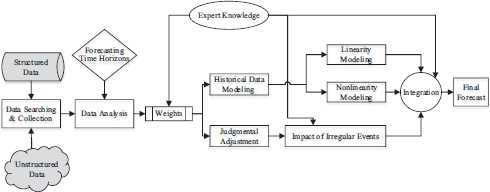
In the proposed air travel demand forecasting framework in Figure 3.6, there are basically three phases in the whole forecasting process, which integrate the linearity modeling, nonlinearity modeling, judgmental adjustment and expert knowledge in an adaptive manner.

In the first phase, the main tasks are data searching and collection, and data analysis. We should collect historical data and related information as much as possible from both the structured data sources and unstructured data sources, as long as it is valuable to the prediction. Then, based on the forecasting time horizons, determine a proper weight for historical data modeling as well as the judgmental adjustment. In the second phase, we step into the main part of a demand forecasting process, i.e., data modeling. There are three main tasks in this phase, including the linearity modeling with a linear forecasting model such as the ARIMA model, the nonlinearity modeling with a nonlinear forecasting model such as the ANN model and determining the impact of irregular events with expert knowledge. In the final phase, the forecasting result from different parts will be integrated to a final forecast with some integration methods. Note that the expert knowledge is utilized in the whole forecasting process with knowledge management techniques. For example, in the ‘Data Analysis’ stage, when a specific forecasting time horizon is required, the weights for ‘Historical Data Modeling’ and ‘Judgmental Adjustment’ are determined by expert knowledge. All studies in the rest of this book are guided by the basic idea of this forecasting framework.

3.3 Common forecasting models

Based on the earlier introduction of TEI@I methodology in the chapter, we introduce and describe the common forecasting models and methods in this section. Firstly, we introduce the use of the econometrical linear forecasting module from a perspective of time series forecasting, and present some common time series models. Secondly, artificial intelligence techniques, as the tools for nonlinearity modeling, are introduced in detail. And at last, we will also cover the main points in implementing combination forecasting and judgmental adjustment with expert knowledge, which are both key parts in the TEI@I methodology.

3.3.1 Econometrical models

Econometrical models consist of massive modeling techniques and methods, and they play a vital role in the forecasting processing of TEI@I methodology. The word ‘econometrics’ was initially proposed by a Norwegian economist Ragnar Frisch in the year 1926. He just got the idea from the word ‘biometrics’, and defined the econometrics as a combination of economics, mathematics and statistics.

Guided by the economic theories and based on the facts, econometrics is a discipline studying the quantitative rule and relationship between economic activities by some mathematical and statistical methods, mostly with the help of computer techniques. In those studying processes, many econometrical models are applied and constructed for the quantitative modeling purposes. In terms of the research contents, econometrics could be classified into two main groups, i.e., theoretical econometrics and applied econometrics. The former focuses the exploration of new econometrical models and methods, while the latter mainly deals with empirical studies to discover the economic operation rule. The econometrical model is the key element for this discipline. Common categories of econometrical models are listed in Table 3.2.

Air travel demand is a typical time series and demonstrates various times series characteristics, such as the randomness and tendency. Hence, to forecast the air travel demand, time series models are the most appropriate and also the most popular in related literature. Generally, time series models can be further divided into several types according to the data patterns, including ARMA models for the stationary time series, ARIMA models for the nonstationary time series, SARIMA models for the nonstationary time series with significant seasonality, VAR models for a vector of stationary time series, VEC models for a vector of stationary time series with significant cointegration relationship among those time series and the ARCH/GARCH family of models for the time series with heteroscedastic random terms.

Table 3.2 Common categories of econometrical models

Classification criterion	Category
The number of variables	Univariate models / multivariable models
The number of equations	Single equation models / simultaneous equations models
The structure of sample data	Cross-sectional models / panel data models / time series models

The use of econometrical models within the TEI@I methodology can be grouped as the applied econometrics. Next, we will describe several main types of econometrical models in detail.

1) ARIMA/SARIMA models

In practice, ARIMA models are one of the most popular econometrical models due to their great modeling performance and the low-cost implementation process. The basic form of ARIMA (p,d,q) models can be described as the following formulations:

$\{\begin{array}{l}\varphi \left(B\right){\nabla }^d{y}_t=\theta \left(B\right)e_t\\ E\left(e_t\right)=0,Var\left(e_t\right)={\sigma }_e^2,E\left(e_t{e}_s\right)=0fors\ne t\\ {\varphi }_p\left(B\right)=1-{\varphi }_{1}B-\cdots -{\varphi }_p{B}^p\\ {\theta }_q\left(B\right)=1-{\theta }_{1}B-\cdots {\theta }_q{B}^q\end{array}$

(3.5)

An earlier section has described the ARIMA models in detail as well as the estimation processes. Hence, we won’t repeat the details here again. The discussion of ARIMA models in Eq. (3.5) are restrictedly applied to non-seasonal time series data. However, the ARIMA models are also capable of modeling the seasonal historical data by adding some additional seasonal terms in Eq. (3.5). In this section, we extend the ARIMA (p,d,q) models of Eq. (3.5) to a seasonal ARIMA model, named the SARIMA (p,d,q)(P,D,Q)^s models, where (p,d,q) denotes the orders of non-seasonal terms and (P,D,Q)^s denotes the orders of the seasonal terms, and s denotes the number of periods per season. The basic SARIMA (p,d,q)(P,D,Q)^s formulations can be written as follows:

$\Phi \left(B^s\right)\varphi \left(B\right){\nabla }_s^d{\nabla }^d{y}_t=\Theta \left(B^s\right)\theta \left(B\right)e_t$

(3.6)

where the seasonal terms in Eq. (3.6) marked by a symbol s are very similar to the non-seasonal terms. And the additional seasonal terms are simply multiplied with the non-seasonal terms.

In Eq. (3.6), y_t and e_t are the actual value and random error at time, respectively; B denotes the backward shift operator, i.e., $B{y}_t=y_{t-1}$ , $B^2{y}_t=y_{t-2}$ and so on; for the non-seasonal terms, $\varphi \left(B\right)=1-{\varphi }_{1}B-\cdots -{\varphi }_p{B}^p$ , $\theta \left(B\right)=1-{\theta }_{1}B-\cdots {\theta }_q{B}^q$ , where p, d are integers and often referred to as orders of the non-seasonal terms. ${\nabla }^d$ is the non-seasonal differencing term; while for the seasonal terms, $\Phi \left(B^s\right)=1-{\varphi }_{1s}{B}^s-\cdots -{\varphi }_{Ps}{B}^{Ps}$ , $\Theta \left(B^s\right)=1-{\theta }_{1s}{B}^s-\cdots {\theta }_{Qs}{B}^{Qs}$ , where P, Q are integers and often referred to as orders of the seasonal terms. ${\nabla }_s^d$ is the seasonal differencing term; the random errors, e_t, are assumed to be independently and identically distributed with a mean of zero and a constant variance of ${\sigma }^2$ , i.e., $e_t\sim IID\left(0,{\sigma }^2\right)$ .

Similar to the specification processes of the ARIMA models, a SARIMA model also involves the following five-step iterative cycle:

1. (a) Stationary test of time series, such as unit root testing;
2. (b) Identification of the SARIMA structure;
3. (c) Estimation of the unknown parameters;
4. (d) Goodness-of-fit tests on the estimated residuals; and
5. (e) Forecast future outcomes based on the known data.

This five-step model construction process is typically repeated several times until a satisfactory model is finally selected. Then the final model can be applied for a prediction purpose.

(2) VAR/VEC models

As a generalization version of the univariate autoregressive (AR) models, vector autoregressive (VAR) models are a family of econometrical models usually used to capture the linear interdependencies among multiple time series. Traditional multivariable models, such as the structural models with simultaneous equations, are based on some economic theories and require enough knowledge about variables. This is difficult sometimes and we need a non-structural model to model the interdependencies among variables. Mainly due to this reason, the VAR models are very popular in the literature because of the ability of modeling more than one evolving variable, and the only prior knowledge required is that those variables can be affected by each other intertemporally. A basic VAR (p) model can be formulated as follows:

$y_t=A_1{y}_{t-1}+\cdots +A_p{y}_{t-p}+u_t,t=1,2,\dots T$

(3.7)

where y_t is a k × 1 vector containing k time series variables in time t; u_t is the k × 1 error term in time t ; the k × k vectors A₁, A₂, ... A_p are the parameters of this model to be estimated. For the error term u_t, we have

$\{\begin{array}{l}E\left(u_t\right)=0\\ E\left(u_t{u^{\prime }}_t\right)=\Sigma \\ E\left(u_t{u^{\prime }}_s\right)=0\forall t\ne s\end{array}$

(3.8)

Eq. (3.8) means that, firstly, every error term in a VAR model has a mean of 0; secondly, the contemporaneous covariance matrix of error terms $E\left(u_t{u^{\prime }}_t\right)$ is a positive-semidefinite matrix; and for any nonzero t / s, there is no correlation across time.

Theoretically, the estimation of the parameters in a VAR (p) model requires that all variables in y_t have to be stationary. Then, if the variables in y_t are cointegrated, they can be modeled with a vector error correction (VEC) model. A VEC model is fit to the first differences of the nonstationary variables, with a lagged error correction term added to the model.

Subtracting y_{t = 1} on both sides of Eq. (3.7) and rearranging terms yields the VEC model as follows:

$\Delta y_t=\Pi y_{t-1}+{\Gamma }_1\Delta y_{t-1}+\cdots {\Gamma }_{p-1}\Delta y_{t-p+1}+u_t$

(3.9)

where $\Pi =-\left(I_k-A_1-\cdots -A_p\right)$ , and ${\Gamma }_i=-\left(A_{i+1}+\cdots +A_p\right),i=1,\dots ,p-1$ .

Suppose this matrix has rank r, and any k × k matrix of rank r can be decomposed as a product of two k × r matrices of full column rank. Let α and β denote the two k × r matrices of rank r such that $\Pi =\alpha {\beta }^{\prime }$ . Hence, substituting the matrix $\alpha {\beta }^{\prime }$ for the term Π can yield

$\Delta y_t=\alpha {\beta }^{\prime }{y}_{t-1}+{\Gamma }_1\Delta y_{t-1}+\cdots {\Gamma }_{p-1}\Delta y_{t-p+1}+u_t$

(3.10)

Eq. (3.10) is the so-called VEC model and the term $\alpha {\beta }^{\prime }{y}_{t-1}$ is the lagged error correction term.

(3) ARCH/GARCH models

The autoregressive conditional heteroscedasticity (ARCH) models and the generalized ARCH (GARCH) models have become important tools in the time series analysis, especially for a financial application. They are particularly useful in analyzing and forecasting volatility.

A financial log-return series y_t may demonstrate many stylized facts. For example, y_t is typically heavy-tailed; the squared series $y_t^2$ is usually strongly auto-correlated for many lags; and the series y_t may respond differently to the positive and negative changes. Hence, the common linear time series models (such as ARMA models) would be not appropriate for modeling this type of time series. To construct a stationary nonlinear model for y_t, Engle (1982) proposed an ARCH, in which the conditional variance of y_t evolves as an autoregressive-type process. Then, Bollerslev (1986) and Taylor (1986) independently generalized Engle’s ARCH model, named a GARCH model. A standard GARCH (p, q) model can be formulated as follows:

$\begin{array}{l}{y}_t={\sigma }_t{\epsilon }_t\\ {\sigma }_t^2=\omega +\sum _{i=1}^p{\sigma }_i{y}_{t-i}^2+\sum _{j=1}^q{\beta }_j{\sigma }_{t-j}^2\end{array}$

(3.11)

where the parameters to be estimated satisfy $\omega >0$ , ${\alpha }_i\ge 0$ , ${\beta }_j\ge 0$ ; and the innovation item ${\epsilon }_t$ is independent and identically distributed with $E\left({\epsilon }_t\right)=0$ and $E\left({\epsilon }_t^2\right)=1$ for any time t.

The main idea of a GARCH model described in Eq. (3.11) is that the conditional variance of y_t given all available up to time t = 1, i.e., the term ${\sigma }_k^2$ , has an autoregressive structure and is also positively correlated to the past value of the squared series. The estimation of a GARCH model can be implemented by a quasi maximum likelihood estimation method.

3.3.2 Artificial intelligence techniques

Artificial intelligence techniques are one of the most important components in the framework of the TEI@I methodology. Specifically, the TEI@I methodology forecasting framework is usually applied to analyzing complex systems. And faced with such complex systems, traditional econometrical models are no longer sufficient in modeling and forecasting the nonlinearity. Hence, artificial intelligence techniques are proposed to accomplish the nonlinearity modeling. The typical artificial intelligence techniques applied in related literature mainly include ANN/BPNN, SVM/SVR and GP.

(1) ANN/BPNN techniques

In the year 1987, Lapedes and Farber (1987) offered the first study to apply the artificial neural network (ANN) techniques on nonlinear signal forecasting. After the past decades’ development, ANN models have been widely applied in many fields such as demand forecasting research and have achieved great forecasting performance in literature.

As described in the previous section, the three-layer BPNN models are the most popular in the literature, and a three-layer BPNN with enough nodes in the hidden layer is able to appropriate any function (e.g., Hornik et al., 1989). As Figure 3.5 shows, the BPNN containing lots of nodes can capture the relatively complex relationship. For the detailed algorithms of the BPNN models, one can refer to many studies (e.g., Rumelhart et al., 1985; Kodogiannis and Lolis, 2002; Chiu et al., 1997). Here, we only introduce the key processes and the main challenges when forecasting a time series with a BPNN model. Figure 3.7 shows the forecasting processes with a BPNN model.

Generally, developing a BPNN model for time series forecasting follows the process illustrated in Figure 3.7. As can be seen from Figure 3.7, the flow chart can be divided into four phases. The first phase is data sampling. To develop a BPNN model in a forecasting scenario, the training, validating and testing data need to be collected in the first step. However, the data collected from various data sources must be cleaned according to the corresponding criteria. In some sense, the network’s success mostly depends upon the quality of training data. After the data are collected, the most important task, and also the most challenging job, is the selection of input variables. How to select the best input variables from a bunch of variables is usually not easy.

The second phase is sample preprocessing. It basically includes three steps: data division, data normalization and determination of network architecture. The data division is aimed at separating the original dataset into three subsets, i.e., training set, validation set and testing set, where the training set is mainly for the training of a BPNN, the validation set is used for strengthening the forecasting performance of the BPNN from the training step and the testing set is for a performance testing. The data normalization is required and indispensable especially when the dataset contains variables of different scales. The last step in this phase is the determination of network architecture, to make sure of the basic structure of the networks used for training, validation and testing. For a detailed description of each step, refer to the study of Yu et al. (2003).

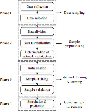
The third phase is the network training and learning. This phase also includes three main tasks, including network initialization, sample training and sample validation. It is the core process of a BPNN forecasting model. In the network initialization process, we should set the original values for several parameters, including the initial connection weight, node bias, learning rate and momentum rate. We usually set those parameters in a random way to avoid the overfitting problem. In the sample training process, some core training algorithms, such as the Levenberg–Marquardt algorithm and the steepest gradient descent algorithm, are often applied in the related literature.

The final phase is the out-of-sample forecasting. When the former three phases are completed, the final BPNN model can be used as a forecaster or predictor for out-of-sample forecasting of time series.

In order to capture the nonlinear characteristics of a specific time series, a BPNN model can be trained by the historical data of a time series. The model parameters (i.e., the connection weights and node biases) will be adjusted iteratively by a process of minimizing the forecasting errors. For a time series forecasting purpose, the final computational form of the BPNN model is

${\hat{y}}_t=a_0+\sum _{j=1}^q{\omega }_{j}f\left(a_j+\sum _{i=1}^p{\omega }_{ij}{y}_{t-i}\right)+{\xi }_t$

(3.12)

where $a_j\left(j=1,2,\cdots ,q\right)$ is a bias on the j th unit, ${\omega }_{ij}\left(i=1,2,\cdots ,p;j=1,2,\cdots ,q\right)$ is the connection weight between nodes in different layers of the BPNN model, $f(·)$ is the transfer function of the hidden layer, p is the number of input nodes and q is the number of hidden nodes. The BPNN model in Eq. (3.12) performs a nonlinear functional mapping from the historical observations $\left(y_{t-1},y_{t-2},\cdots ,y_{t-p}\right)$ to achieve forecasted current value ${\hat{y}}_t$ , as follows:

${\hat{y}}_t=\phi \left(y_{t-1},y_{t-2},\cdots ,y_{t-p},\upsilon \right)+{\xi }_t$

(3.13)

where v is a vector of all parameters and φ is a function determined by the network structure and connection weights. Thus, in some senses, the BPNN model is equivalent to a nonlinear autoregressive (NAR) model. And the objective function in the training process is usually set as

$\min Error=\frac{1}{2}{\Vert y_t-{\hat{y}}_t\Vert }^2=\frac{1}{2}{\Vert y_t-\left(a_0+\sum _{j=1}^q{\omega }_{j}f\left(a_j+\sum _{i=1}^p{\omega }_{ij}{y}_{t-i}\right)+{\xi }_t\right)\Vert }^2$

(3.14)

where y_t is the true value, and ${\hat{y}}_t$ is the forecast achieved by the BPNN model.

Thus, the processes for developing a back-propagation neural network model are listed as follows and were proposed by Ginzburg and Horn (1994).

1. (a) Normalize the learning set;
2. (b) Decide the network architecture and initial parameters: i.e., the nodes bias, learning rate, momentum rate and network architecture. Unfortunately, there are no criteria in deciding the parameters other than a trial-and-error basis;
3. (c) Initialize all weights randomly;
4. (d) Implement a training process, where the stopping criterion is either the number of iterations reached or when the total sum of squares of error is lower than a pre-determined value;
5. (e) Choose the network with the minimum error (i.e., model selection criterion); and
6. (f) Forecast the future outcome.

Readers who are interested in a more detailed introduction of ANN/BPNN modeling techniques can also refer to the related literature (see, e.g., Tang and Fishwick, 1993; Tang et al., 1991; Zhang et al., 2001; Chen and Leung, 2004).

(2) Support vector machines

The shortcomings of a BPNN forecasting model include that the BPNN model has a low convergence rate and is easy to fall into a local minimum trap. Thus, to overcome these shortcomings, researchers proposed another artificial intelligence technique instead, named support vector machines.

First proposed by Vapnik (1995), support vector machines (SVM) are a successful realization of the statistical learning theory (SLT). It is a computational intelligence model based on the SLT’s Vapnik–Chervonenkis theory and the principle of structural risk minimization. A SVM model is seeking a balance between the model’s training precision and forecasting accuracy with limited sample information at hand, in order to obtain a better generalization ability. A SVM model can also be called a support vector regression (SVR) model if it is trained for a regression analysis, or a support vector classification (SVC) model for a classification analysis. The basic idea of a SVM is mapping a nonlinear problem in the low-dimensional feature space to a linear problem of a high-dimensional space, to simplify the problem. The SVM models have been proved to possess excellent capabilities in forecasting even for small samples, whose training is however a time consuming process when facing high-dimensional data. To deal with this problem, Suykens and Vandewalle (1999) proposed a new version of the SVM algorithms, named least squares support vector machine (LSSVM) models. According to the modeling purposes, LSSVM models can also be categorized into two main groups, i.e., least squares support vector regression (LSSVR) and least squares support vector classification (LSSVC) for the regression and classification purposes, respectively. Specifically, the LSSVR models are usually applied in forecasting literature. In this section, we will give a brief description for the SVR models and LSSVR models.

The training dataset is defined as $\left\{x_t,y_t\right\}\left(t=1,2,\cdots ,T\right)$ , where x_t, y_t is t th corresponding input and output. According to the basic idea of a SVR model, firstly, the original input data {x_t} is mapped into a high-dimensional feature space via a nonlinear mapping function, named $\phi (·)$ ; secondly, the output data {y_t} is regressed on $\phi \left(x_t\right)$ in this high-dimensional feature space. And the regression model can be formulated as follows:

${\hat{y}}_t=w^{\prime }\phi \left(x_t\right)+b�t=1,2,\cdots ,T$

(3.15)

where $\phi \left(x_t\right)$ is the nonlinearly mapped value for the input x_t, and ${\hat{y}}_t$ is the estimated value for the output. Coefficients w and b can be obtained by minimizing the regularized risk function and adding two slack variables. The transformed optimization problem is as follows:

$\begin{array}{l}\min \frac{1}{2}{w}^{\prime }w+\gamma \sum _{t=1}^T\left({\xi }_t+{\xi }_t^{\ast }\right)\\ s.t.w^{\prime }\phi \left(x_t\right)+b-y_t\le \epsilon +{\xi }_t^{\ast },\left(t=1,2,\cdots ,T\right)\\ y_t-\left(w^{\prime }\phi \left(x_t\right)+b\right)\le \epsilon +{\xi }_t,\left(t=1,2,\cdots ,T\right)\end{array}$

(3.16)

where γ is a penalty parameter and variables ${\xi }_t^{\ast }$ and ${\xi }_t$ are the slack variables. Obviously, Eq. (3.16) is a quadratic programming problem and may lead to a high computational cost.

Hence, a new version of the SVR models, i.e., the LSSVR models, is proposed to solve this challenging problem by using a set of linear regression equations instead of the constraint conditions in Eq. (3.16). Thus, the optimization problem in Eq. (3.16) of the SVR models can be transformed into the following LSSVR model:

$\begin{array}{l}\min \frac{1}{2}{w}^{\prime }w+\frac{1}{2}\gamma \sum _{t=1}^T{e}_t^2\\ s.t.y_t=w^{\prime }\phi \left(x_t\right)+b+e_t\left(t=1,2,\cdots ,T\right)\end{array}$

(3.17)

where e_t indicates the slack variable. Eq. (3.17) is the optimization problem in a LSSVR model.

With the help of Lagrangian method and Karush-Kuhn-Tucker conditions for optimality, the solution to Eq. (3.17) can be represented as

$\hat{y}=\sum _{t=1}^T{w}^{\prime }K\left(x,x_t\right)+b$

(3.18)

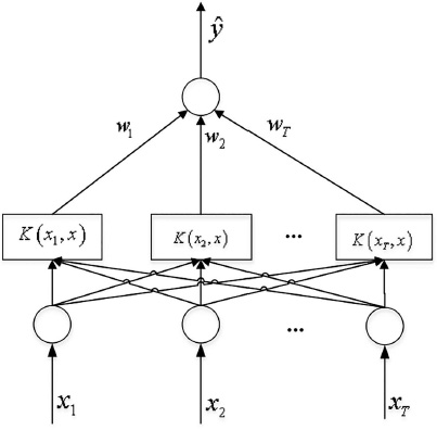
In Eq. (3.18), $K(·)$ represents the kernel function to simplify the mapping process. Usually, a symmetric kernel function $K(·)$ which satisfies Mercer’s condition corresponds to a dot product in some feature spaces. And in practice, the most popular kernel functions include the Gaussian kernel function $K\left(x,x_t\right)=\exp \left(\Vert x-x_t\Vert /2{\sigma }^2\right)$ with a parameter of σ, and the polynomial kernel function $K\left(x,x_t\right)={\left(a_{1}x{x}_t+a_2\right)}^d$ with an order of d and the constants a₁ and a₂. Figure 3.8 demonstrates a simple estimation process of Eq. (3.18).

(3) Genetic programming

Genetic programming (GP) is an evolutionary algorithm-based methodology to figure out the mathematical equations which perform a user-defined task best. First proposed by Koza (1992), GP operates mathematical equations in the form of trees which comprise the sequence functions and their arguments are placed in subsequent nodes. Figure 3.9 illustrates a tree representing a simple expression of x × x + y/2.

The basic processes of a GP model are similar to that of the genetic algorithm (GA). And the main operators in the GP models are reproduction, crossover and mutation similar to those in the GA models. Basically, the GP model starts with an initial population and ends with the best one. Firstly, an initial population is set. Secondly, in the training process, the GP model reproduces and makes new generations based on a predefined fitness function, where the crossover operator is to switch nodes in a population, and the role of a mutation operator is to take and replace the information of some node. A new generation will also be evaluated by the fitness function.

This loop continues until the fitness reaches the predefined threshold. More details of GP can be found in Koza (1992).

3.3.3 Combination forecasting method

Every single model has its own advantages and disadvantages, and should be developed according to the specific forecasting problems and actual conditions. Given the complexity of the real world, there is no single model that can perform well under all situations. So here is a straight thought: what if we combine the forecasts of several single forecasting models to form a final combined forecast; maybe in this way we could achieve a better forecast than that of a single model. This combination forecasting technique had been proven to be a right and effective forecasting technique. Many studies (e.g., Armstrong, 2001; Yu, 2005) believed that a combination forecasting model could generate a better forecast than a single forecasting model, if these constitutive models in a combination forecasting model were all precise and diversified enough.

The core idea of the combination forecasting methods is to combine various individual forecasts from multiple single forecasting models, and then to achieve a better combined forecast. Thus, the key question in this forecasting process is how to combine the single forecasting models and then how to decide the weights for each constitutive forecasting model. Basically, the combination approaches can be classified into two groups, i.e., linear combination forecasting and nonlinear combination forecasting. At present, the majority of the existing combination approaches belong to the former group.

(1) Linear combination approach

The linear combination approaches usually include a simple averaging approach and a weighted averaging approach according to the method used for determining weights.

The simple averaging approach is the simplest and the most common method used in the combination forecasting method. This approach can be simply described as follows. If there are m individual forecasts to be combined, then assign the weight as l/m for each individual forecast. Some studies (e.g., Hansen and Salamon, 1990; Breiman, 1994) had proved that the simple averaging approach was an effective way to improve the forecasting performance. The simple averaging approach is simple and effective; however, weighting every individual model equally sometimes is not appropriate due to the different forecasting performance of each individual model.

To improve the simple averaging approach, the weighted averaging approach is proposed and highly recommended in the literature. This approach determines the weights based on the forecasting performance of each individual forecasting model. There are three popular weighted averaging approaches, including the mean squared error method (see Benediktsson, 1997), the stacked regression method (see Breiman, 1996) and the variance-based weighted method (Tresp and Taniguchi, 1995). For the mean squared error method, the weights are chosen by minimizing the mean squared error, i.e., for any t = 1,2,&,T,

$\{\begin{array}{l}{w}_t^{opt}=\arg \underset{w_t}{\min }\left\{{\sum }_{j=1}^m{\left({w^{\prime }}_t{f}_t\left(x_j\right)-d_{jt}\left(x_j\right)\right)}^2\right\}\\ {\sum }_{t=1}^T{w}_t=1;w_t\ge 0\end{array}$

(3.19)

Suppose there are m individual models; the $w_t^{opt}$ in Eq. (3.19) denotes the optimal weight vector in time t; $f_t\left(x_j\right)$ is the final forecast obtained by the j th individual model and $d_{jt}\left(x_j\right)$ is the corresponding target value. Then Eq. (3.19) calculates the weights by minimizing the squared error.

Breiman (1996) also proposed a modified mean squared error method, named the stacked regression method, to improve the performance of the mean squared error method. The objective function can be transformed as follows, for any t = 1,2,...,T:

$\{\begin{array}{l}{w}_t^{opt}=\arg \underset{w_t}{\min }\left\{{\sum }_{j=1}^m{\left({w^{\prime }}_t{g}_t\left(x_j\right)-d_{jt}\left(x_j\right)\right)}^2\right\}\\ {\sum }_{t=1}^T{w}_t=1;w_t\ge 0\end{array}$

(3.20)

where $g_t\left(x_j\right)\text{=}\left(f_t^{\left(1\right)}\left(x_j;D_{cv}\right),\dots ,f_t^{\left(m\right)}\left(x_j;D_{cv}\right)\right)$ is a cross-validation version of $f_t\left(x_j\right)$ , and D_cv is the cross-validation dataset.

The last weighting approach is called the variance-based weighted approach, and the objective function is as follows, for any t = 1,2,...,T:

$\{\begin{array}{l}{w}_t^{opt}=\arg \underset{w_t}{\min }\left\{{\sum }_{t=1}^n\left(w_t{\sigma }_t^2\right)\right\}\\ {\sum }_{t=1}^T{w}_t=1;w_t\ge 0\end{array}$

(3.21)

With Lagrange’s theorem, the optimal weight is as follows:

$w_t^{opt}=\frac{{\left({\sigma }_t^2\right)}^{-1}}{{\sum }_{t=1}^n{\left({\sigma }_t^2\right)}^{-1}},t=1,2,\dots T$

(3.22)

(2) Nonlinear combination approach

Besides those simple averaging methods and weighted averaging methods, the nonlinear weighted averaging methods based on the artificial intelligence techniques such as the BPNN and SVM (e.g., Brown et al., 2005; Yu et al., 2008; Xie et al., 2013) are also popular and constitute a major trend in assigning weights.

Here is a simple introduction of the nonlinear weighted averaging methods based on SVM techniques. Generally, in the SVM-based weighting scheme, the final combined forecast is considered as a dependent variable, and a functional relationship between the final combined forecasts and those individual forecasts should be estimated by the SVM techniques. The function can be formulated as follows:

$y=f\left(x\right)+\epsilon$

(3.23)

where y is the combined forecast to be calculated; x2 is a vector containing various individual forecasts; and $f(·)$ denotes some deterministic function, which can be determined by a SVR model. The detailed estimation process for Eq. (3.23) is similar with that in a forecasting application (see Figure 3.8), and the estimated parameters are the weights for various individual forecasting models.

3.3.4 Expert knowledge and judgmental adjustment

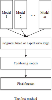
Expert knowledge plays a vital role in demand forecasting especially for a relatively long forecasting time horizon. So, how to incorporate the expert knowledge into a mathematical forecasting method attracts much researcher attention. In general, there are four basic methods of incorporating expert knowledge (see Figure 3.10).

In the first method, the individual forecasts from every single forecasting model are firstly adjusted by the experts’ judgment with their experience and domain knowledge. Then the adjusted forecasts are combined with some combination forecasting techniques to obtain a final forecast. This method makes full use of the expert knowledge because experts should be involved in adjusting the forecast from every forecasting step. However, the biggest disadvantage is that it costs a lot of those experts’ time and energy in doing this job; especially when the forecasting frequency is at a high level, this method would become infeasible due to this disadvantage (Davydenko and Fildes, 2012).

In the second method, the individual forecasts from every single forecasting model are firstly combined and the combined forecast is then adjusted by the experts with their experience and domain knowledge. This method is the easiest to implement in reality; however, the subjectivity of the experts’ judgments will easily result in a subjective bias and inconsistency. Researchers discussed the problem and proposed several solutions to that in related literature. They believed that the group decision technique can effectively solve this problem (e.g., Lawrence et al., 1986; Sniezek, 1989), and also Sniezek (1989) concluded that the type of group decisions adopted actually had little influence on the final forecast, while some other studies such as Brenner, Griffin and Koehler (2005) showed that the group decision technique would, to some extent, induce the participants to pay more attention to that positive information, being more prone to generate relatively high forecasts consequently. Thus, they concluded that the Delphi methods with no interaction between experts would perform more steadily and effectively.

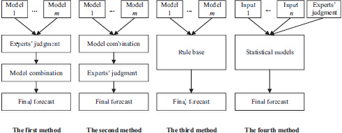
The third method is based on a rules base. By using this method, the first job is to transfer the experts’ knowledge into rules, then these rules can be used as a reference basis for judgmental adjustment in a forecasting process. However, maintaining a rules base is usually costly and a main drawback of this method is that the updating of rules is not timely most of the time (Davydenko and Fildes, 2012), thus the rules base cannot reflect the newest information and knowledge.

In the former three methods of incorporating expert knowledge, the similarity is that the experts adjust the forecasts directly with their knowledge and experience. Different from the former three methods, the fourth one emphasizes the integration of expert knowledge and the whole forecasting process. It mainly considers the expert knowledge as an important input for the forecasting model, and lets the expert knowledge function in almost every forecasting stage (e.g., West and Harrison, 1989; Yelland et al., 2010 and etc.). Huang (2014) has discussed the fourth method in detail (see Figure 3.11).

He described that a whole forecasting process is mainly consisting of the variable selection, data preprocessing, model construction, model estimation and forecasts selection, where the expert knowledge can function in every step. Take the variable selection and data preprocessing, for example.

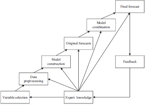
1. (a) Analyzing the relationship between the explained variable and the explanatory variables. An effective forecasting model should be able to describe the core relationship between variables. To meet this requirement, experts’ knowledge and experience play an irreplaceable role in examining the relationships and are helpful in determining the optimal variable set.
2. (b) Selecting the appropriate explanatory variables. In reality, an economic phenomenon usually can be described by more than one variable. Therefore, the selection of the proper variable in this situation is largely based on the experts’ judgment. In addition, to avoid the endogeneity problem, satisfying instrumental variables are required. These challenging tasks are usually accomplished by the domain experts based on their theoretical knowledge and forecasting experience.
3. (c) Outliers detection and handling. The original dataset usually contains some outliers, including the missing values, erroneous records and other types of outliers. Outliers should not be removed roughly by some statistical programs, without any further investigation. To deal with the outliers carefully, expert knowledge is necessary in outlier detection and judgment.

3.4 Conclusions

In this chapter, we introduced the theoretical basis of this book, i.e., TEI@I methodology. Firstly, we discussed the motivation of TEI@I methodology from a theoretical point of view. The TEI@I methodology was originally proposed for analyzing complex systems, due to their inherent complexity and nonlinearity. Secondly, we described the framework of TEI@I methodology in detail. The framework of TEI@I methodology mainly consists of six function modules, including the man-machine interface module, the web-based text mining module, rule-based expert system module, ARIMA-based econometrical linear forecasting module, ANN-based nonlinear forecasting module and the bases and bases management module. And then based on the general framework of TEI@I methodology, we proposed an integrated air travel demand forecasting framework as a unified guide for forecasting modeling.

After introducing the theoretical framework and the air travel demand forecasting framework, we also briefly covered several common forecasting methods and models. Firstly, we introduced the use of econometrical forecasting models in time series forecasting, and presented several common models such as ARIMA/SARIMA models, VAR/VEC models and ARCH/GARCH models. Secondly, for nonlinearity modeling, several artificial intelligence techniques, including the ANN, SVR/LSSVR and GP, were introduced briefly. Finally, we also covered the main points in implementing combination forecasting and judgmental adjustment with expert knowledge, which are both key parts in the TEI@I methodology. Note that there are several key problems involved in the combination forecasting technique, which is a key process in our forecasting framework.

Firstly, in a combination forecasting process, the first task is to construct several individual forecasting models for a combination purpose. However, the selection of those individual forecasting models usually causes some confusion for both researchers and practitioner. The basic question is whether combining some homogeneous models or combining some heterogeneous models would perform better. The study of Krogh and Sollich (1997) concluded that, if the individual forecasting models were heterogeneous and uncorrelated, the forecasting performance of the final combination forecasting model would be improved significantly. Yu (2005) applied a bias-variance decomposition method to explore this selection question. The results showed that homogeneous models tend to generate correlated forecasting errors, thus making it difficult to reduce the total forecasting error; while the heterogeneous models can generate uncorrelated forecasting error, and the final forecasting error could be reduced through a combination technique. Yu finally came to a conclusion that the forecasting performance of a combination model based on heterogeneous forecasting models was better than using the homogeneous models.

Secondly, in a combination forecasting process, other questions include whether more individual forecasting models combined would mean a better performance, and how to determine an optimal number of individual forecasting models. Actually, some studies have discussed these questions in detail. For example, Yu (2005) achieved a conclusion that when there were a bunch of individual forecasting models at hand, combining a part of them would be very likely to perform better than combining all of those individual forecasting models. Then Yu proposed a method based on minimizing conditional generalized variance, to determine the optimal number of individual models. In practice, we usually determine the number based on many factors, including the acceptable forecasting cost, forecasting accuracy required, etc.

References

Armstrong, J. S. (Ed.). (2001). Principles of Forecasting: A Handbook for Researchers and Practitioners. New York, Springer Science & Business Media.
Benediktsson, J. A., Sveinsson, J. R., Ersoy, O. K., and Swain, P. H. (1997). Parallel consensual neural networks. IEEE Transactions on Neural Networks, 8(1), 54–64.
Bollerslev, T. (1986). Generalized autoregressive conditional heteroskedasticity. Journal of Econometrics, 31(3), 307–327.
Box, G. E., and Jenkins, G. M. (1970). Time Series Analysis: Forecasting and Control. San Francisco, Holden-Day.
Breiman, L. (1994). Bias, Variance, and Arcing Classifiers. Technical Report TR 460, Department of Statistics, University of California.
Breiman, L. (1996). Stacked regressions. Machine Learning, 24(1), 49–64.
Brenner, L., Griffin, D., and Koehler, D. J. (2005). Collaborative planning and predication: Does group discussion affect optimistic case-based judgment. Organizational Behavior and Human Decision Processes, 97(1), 64–81.
Brown, G., Wyatt, J. L., and Tiňo, P. (2005). Managing diversity in regression ensembles. Journal of Machine Learning Research, 6(Sep), 1621–1650.
Buehler, R., Messervey, D., and Griffin, D. (2005). Collaborative planning and prediction: Does group discussion affect optimistic biases in time estimation? Organizational Behavior and Human Decision Processes, 97(1), 47–63.
Chen, A. S., and Leung, M. T. (2004). Regression neural network for error correction in foreign exchange forecasting and trading. Computers & Operations Research, 31(7), 1049–1068.
Chiu, C. C., Kao, L. J., and Cook, D. F. (1997). Combining a neural network with a rule-based expert system approach for short-term power load forecasting in Taiwan. Expert Systems with Applications, 13(4), 299–305.
Davydenko, A., and Fildes, R. (2012). A Joint Bayesian Forecasting Model of Judgment and Observed Data. Working Paper, The Department of Management Science, Lancaster University.
Denton, J. W. (1995). How good are neural networks for causal forecasting? The Journal of Business Forecasting, 14(2), 17.
Engle, R. F. (1982). Autoregressive conditional heteroscedasticity with estimates of the variance of United Kingdom inflation. Econometrica: Journal of the Econometric Society, 50(4), 987–1007.
Ginzburg, I., and Horn, D. (1994). Combined neural networks for time series analysis. Neural Information Processing Systems, 6, 224–231.
Ginzburg, I., and Horn, D. (1994). Combined Neural Networks for Time Series Analysis. Proceedings of the Neural Information Processing Systems Conference.
Hansen, L. K., and Salamon, P. (1990). Neural network ensembles. IEEE Transactions on Pattern Analysis and Machine Intelligence, 12(10), 993–1001.
Hornik, K., Stinchcombe, M., and White, H. (1989). Multilayer feedforward networks are universal approximators. Neural Networks, 2(5), 359–366.
Huang, A. Q. (2014). Research on Forecasting Method of Seaport Container Throughput and Airport Transport Demand. The PHD Dissertation of Beijing University of Aeronautics and Astronautics, Beijing, China.
Kodogiannis, V., and Lolis, A. (2002). Forecasting financial time series using neural network and fuzzy system-based techniques. Neural Computing & Applications, 11(2), 90–102.
Koza, J. R. (1992). Genetic Programming: On the Program of Computer by Natural Selection. Cambridge, MA, MIT Press.
Krogh, A., and Sollich, P. (1997). Statistical mechanics of ensemble learning. Physical Review E, 55(1), 811.
Krogh, A., and Vedelsby, J. (1995). Neural network ensembles, cross validation, and active learning. Proceedings of Neural Information Processing Systems. Cambridge, MA, MIT Press.
Lapedes, A., and Farber, R. (1987). Non-Linear Signal Processing Using Neural Network: Prediction and System Modelling. Technical Report LA_UR-87–2662, Los Alamos National Laboratory.
Lawrence, M. J., Edmundson, R. H., and O’Connor, M. J. (1986). The accuracy of combining judgemental and statistical forecasts. Management Science, 32(12), 1521–1532.
MacQueen, J. (1967). Some Methods for Classification and Analysis of Multivariate Observations. Proceedings of the 5th Berkeley Symposium on Mathematical Statistics and Probability, California, USA.
Markham, I. S., and Rakes, T. R. (1998). The effect of sample size and variability of data on the comparative performance of artificial neural networks and regression. Computers & Operations Research, 25(4), 251–263.
Olson, C. F. (1995). Parallel algorithms for hierarchical clustering. Parallel Computing, 21(8), 1313–1325.
Rajman, M., and Besançon, R. (1998). Text Mining-Knowledge Extraction from Unstructured Textual Data. Proceedings of the 6th Conference of International Federation of Classification Societies, Rome, Italy.
Rumelhart, D. E., Hinton, G. E., and Williams, R. J. (1985). Learning Internal Representations by Error Propagation. California Univ San Diego La Jolla Inst for Cognitive Science, No. ICS-8506.
Rumelhart, D. E., and Mcclelland, J. L. (1986). Parallel Distributed Processing: Explorations in the Microstructure of Cognition. Cambridge, MA, MIT Press.
Salton, G., Wong, A., and Yang, C. S. (1975). A vector space model for automatic indexing. Communications of the ACM, 18(11), 613–620.
Shi, Z. (2002). Knowledge Discovery. Beijing, China, Publishing House of Tsinghua University.
Sniezek, J. A. (1989). An examination of group process in judgmental forecasting. International Journal of Forecasting, 5(2), 171–178.
Suykens, J. A., and Vandewalle, J. (1999). Least squares support vector machine classifiers. Neural Processing Letters, 9(3), 293–300.
Tang, Z., de Almeida, C., and Fishwick, P. A. (1991). Time series forecasting using neural networks vs Box-Jenkins methodology. Simulation, 57(5), 303–310.
Tang, Z., and Fishwick, P. A. (1993). Feedforward neural nets as models for time series forecasting. ORSA Journal on Computing, 5(4), 374–385.
Taylor, S. J. (1986). Modelling Financial Time Series. Chichester, UK, Wiley.
Tian, X., Lu, X. S., and Deng, X. M. (2009). A TEI@I-Based Integrated Framework for Port Logistics Forecasting. Proceedings of International Conference on Business Intelligence and Financial Engineering, Beijing, China.
Tresp, V., and Taniguchi, M. (1995a). Combining Estimators Using Non-Constant Weighting Functions. Proceedings of Neural Information Processing Systems.
Tresp, V., and Taniguchi, M. (1995b). Combining estimators using non-constant weighting functions. In: Tesauro, G., Touretzky, D., and Lean, T. (eds.), Advances in Neural Information Processing Systems. MIT Press, Cambridge, MA, 419–426.
Vapnik, V. (1995). The Nature of Statistical Learning Theory. New York: Springer Verlag.
Wang, S. Y. (2004). TEI@I: A New Methodology for Studying Complex Systems. Proceedings of the International Workshop on Complexity Science, Tsukuba, Japan.
Wang, S. Y., Yu, L., and Lai, K. K. (2005). Crude oil price forecasting with TEI@I methodology. Journal of Systems Sciences and Complexity, 18(2), 145–166.
Wang, S. Y., Yu, L. A., and Lai, K. K. (2007). TEI@ I methodology and its application to exchange rates prediction. Chinese Journal of Management, 4(1), 21–26.
West, M., and Harrison, J. (1989). Subjective intervention in formal models. Journal of Forecasting, 8(1), 33–53.
Xie, G., Wang, S., and Lai, K. K. (2013). Air Passenger Forecasting by Using a Hybrid Seasonal Decomposition and Least Squares Support Vector Regression Approach. DOI: http://2013.isiproceedings.org/Files/CPS205-P37-S.pdf
Yan, Y., Wei, X., Hui, B., Yang, S., Zhang, W., Hong, Y. U. A. N., and Wang, S. Y. (2007). Method for housing price forecasting based on TEI@I methodology. Systems Engineering-Theory & Practice, 27(7), 1–9.
Yelland, P. M., Kim, S., and Stratulate, R. (2010). A Bayesian model for sales forecasting at Sun microsystems. Interfaces, 40(2), 118–129.
Yu, L. A. (2005). Forecasting Foreign Exchange Rates and International Crude Oil Price Volatility Within TEI@I Methodology. The PHD Dissertation of Chinese Academy of Sciences, Beijing, China.
Yu, L. A., Wang, S. Y., and Lai, K. K. (2003a). A hybrid AI system for forex forecasting and trading decision through integration of artificial neural network and rule-based expert system. Expert System with Applications, 14(1), 433–441.
Yu, L. A., Wang, S. Y., and Lai, K. K. (2003b). An Integrated Framework for a BPNN-Based for Ex Rolling Forecasting System and Web-Based for Ex Trading Decision Support System. Submitted to Decision Support Systems.
Yu, L. A., Wang, S., and Lai, K. K. (2008). Forecasting crude oil price with an EMD-based neural network ensemble learning paradigm. Energy Economics, 30(5), 2623–2635.
Zhang, G. P. (2003). Time series forecasting using a hybrid ARIMA and neural network model. Neurocomputing, 50, 159–175.
Zhang, G. P., Patuwo, B. E., and Hu, M. Y. (2001). A simulation study of artificial neural networks for nonlinear time-series forecasting. Computers & Operations Research, 28(4), 381–396.