6   A novel seasonal decomposition-based short-term forecasting framework with Google Trends data

For monthly and quarterly historical data, seasonality is one of the most significant data patterns. When predicting the future demand, it is essential to measure and adjust the seasonality in order to understand the underlying historical trends more precisely. However, it is difficult for the existing seasonality analysis procedures to precisely deal with the seasonality adjustment on every economic time series, due to the individual characteristics of every time series, especially for the moving holiday effects. Therefore, in the short-term air travel demand forecasting, we usually encounter a poor forecasting performance problem for those months suffering moving holiday effects, especially for those popular and important holidays that have a strong influence on the passengers’ flying behaviors. For example, the Chinese New Year holiday is one of the most important public holidays, and during the Chinese New Year holiday, people will travel much more than ordinary times. However, because of the holidays, a great demand forecasting performance for these related months becomes more necessary, to guarantee a smooth operation in these days.

In this chapter, to deal with this tough forecasting problem, we propose a forecasting framework based on the seasonal decomposition method with a novel use of Google Trends data. Section 6.1 introduces the research background and motivations briefly; section 6.2 summarizes common approaches to capture the moving holiday effects and propose a new method for capturing the moving holiday effects. We also provide an empirical analysis and comparison between the common approach and our proposed method; then section 6.3 proposes a forecasting framework based on the former analysis, and section 6.4 demonstrates a nowcasting process with higher-frequency information; and section 6.5 concludes this chapter.

6.1 Introduction

In a time series, the seasonality is defined as the presence of data variations that occur at some regular intervals, such as quarterly, monthly or even weekly. Seasonality is usually caused by various factors such as holiday effects, the weather, etc., which may result in totally different consuming behaviors. Those periodic, repetitive, regular and predictable patterns in the time series are relatively easy to capture. However, for those moving holiday effects, it is not easy to capture and adjust with the existing procedures, and the moving holiday effects are usually ignored directly by most researchers.

When implementing a short-term air travel demand forecasting with monthly or quarterly historical data, seasonality is one of the most significant data patterns. To achieve a good forecasting performance, the seasonality should be carefully measured and adjusted in order to understand the underlying trends when forecasting the future demand. This purpose raised the importance of the seasonal adjustment. A seasonal adjustment is any method that can remove the seasonal component out of a time series. The main objective of seasonal adjustment can be stated as ‘to simplify the data so that they may be more easily interpreted … without a significant loss of information’ (Bell and Hillmer, 1984). The most popular methods for seasonal adjustment can be classified into two groups, i.e., the parametric (or model-based) methods and the non-parametric methods. The first group of seasonal adjustment methods is usually developed based on parametric models, such as the SARIMA models. This group mainly includes the TRAMO/SEATS method developed by Bank of Spain and the STAMP method developed by Andrew Harvey. The TRAMO/SEATS method, using the ARIMA model as its basis for seasonal adjustment, is widely used worldwide. The second group of seasonal adjustment methods mainly includes the X-11 family developed by the US Census Bureau, and the SABL and STL methods developed by Bell Labs, where the X-11 family is the most popular seasonal adjustment in related literature and also in practice. The latest version of an X-11 method is named the X-13-ARIMA-SEATS method, which combines both X-11 and SEATS modules to provide comprehensive seasonal adjustment functions. Generally, understanding and capturing the seasonal patterns and underlying trend component are extremely important for any empirical economic analysis, including the short-term air travel demand forecasting in this chapter.

Among all calendar effects faced in the seasonal adjustment process, the moving holiday effect is the most difficult to quantify. Take the Chinese economic time series, for example. The Chinese New Year (CNY) holiday is the most important holiday that has great influence on almost every Chinese economic activity. However, the specific date of the Chinese New Year’s Day in every year is moving between January 21 and February 20 in the Gregorian calendar, which could explain the name of ‘moving holiday effect’. Having strong influence on economic activities occurring in January and February, the CNY effect usually makes the common seasonal adjustment method misleading and in turn results in a biased empirical finding. In the research of short-term air travel demand forecasting, we have found that the forecasting errors for Januarys and Februarys are usually larger than for other months. This is mainly due to the moving holiday effects, i.e., the CNY effect to a great extent.

However, in the literature of air travel demand forecasting research, seasonal adjustments have been usually implemented by the popular methods in the X-11 family or TRAMO/SEATS software with the default settings, but few people have ever discussed the data-specific seasonal characteristics such as a CNY holiday effect. Even though several built-in options are provided for the users to deal with the trading day effect and holiday effects such as the Easter holiday, Thanksgiving holiday, etc., an approach to manage the general moving holiday effects is still lacking. This is one big problem that we should deal with in the first place when doing short-term air travel demand forecasting.

Therefore, in this chapter, we will mainly deal with the difficult forecasting problem for those periods influenced by the moving holiday effects, and propose a forecasting framework based on a seasonal decomposition method and a novel use of Google Trends data, which are taken as the exogenous variables to capture the moving holiday effects. The air passenger traffic of HKIA is taken as the historical data for an empirical analysis, where the CNY holiday effect is our concern in this chapter. The proposed method can not only solve the tough forecasting problem for those holiday periods, but also demonstrates superior forecasting performance in other forecasting time horizons. Firstly, to model specific moving holiday effects accurately, we will introduce two types of exogenous variables to capture the holiday effects based on either the holiday calendar or the Google Trends data, and then provide an empirical comparison for the two types of exogenous variables. The results show that constructing the exogenous variables with the Google Trends data, i.e., the users’ search data with proper keywords, is a better way to model the moving holiday effect. Secondly, we will propose a forecasting framework based on the seasonal decomposition method with the novel use of Google Trends data as the exogenous variables to capture the moving holiday effect. In addition, we will also present a nowcasting process in detail with weekly Google Trends data by adopting a MIDAS model, to show that the information with a higher frequency can effectively help to improve the forecasting accuracy.

6.2 Genhol vs. Google Trends

In related literature, the moving holiday effect on each day within a user-defined holiday interval is generally assumed to be equal and constant, and the holiday effect regressor for a given month is defined as the proportion of the holiday interval that falls in this month (e.g., Lin and Liu, 2002). This approach had been adopted in the methods of the X-11 family. Take the construction approach for an Easter holiday regressor in the X-13-ARIMA-SEATS method, for example; the regressor can be defined as follows:

where w is the number of days in a user-defined holiday interval before the Easter holiday, and n_t is the number of days in the user-defined holiday interval that fall in month t (for monthly data). The value of this regressor would be 0 except in February, March and April, and it is a nonzero in February only for w > 22. The final length of the holiday interval, i.e., w, is determined by some criteria of modeling performance, e.g., Akaike Information Criteria (AIC) and out-of-sample forecasting performance. Note that this is just a simple example of the before-holiday effect. According to the specific characteristics of each time series, we can also construct regressors for the during-holiday effect and the after-holiday effect in the meantime. In those existing seasonal adjustment programs, there are no built-in Chinese-specific holiday regressors. Therefore, researchers usually ignore the Chinese-specific moving holiday effects when doing an empirical analysis on a Chinese economic time series. Luckily, there is a Genhol program provided by the X-13-ARIMA-SEATS team that can be used to generate any user-defined moving holiday regressors as Eq. (6.1) by providing every year’s holiday date.

However, the equal-weight assumption for each day’s holiday effect in the predefined holiday intervals is often not necessarily true in reality; and the length of holiday intervals is not necessarily equal for every single year, because air passengers’ flying behaviors will be influenced by many factors that are changing year by year. To deal with these two drawbacks, we propose a novel method with the use of Google Trends data, to model the moving holiday effects on air travel demand.

Web search data from the search engines has been proven to be a great predictor of macroeconomic activities (e.g., Goel et al., 2010; Choi and Varian, 2012; Wu and Brynjolfsson, 2015). The main reason for this connection between the web search data and macroeconomic activities would be that those search data connect closely with users’ daily life and can reflect the users’ opinions and interests on economic events. Generally, web search data are defined as search volumes of a specific term or phrases via search engines during a period of time. A larger search volume tends to represent more attention and interest on this subject from the users, thus it could be used to help forecast demand to a great extent. Among all famous search engines, Google is the most popular with about 65.2 percent market share according to the comScore marketing research, so the search data from Google are more representative than other search engines. As a public tool, Google Trends provides time sequence search data by dividing the count of each search keyword by total online search queries which are submitted during that week. The Google Trends data are available at a weekly or monthly frequency since January 2004. Hence, the Google Trends data can provide a comprehensive and feasible way to measure the public opinions and interests, and are therefore considered as another important data source for the economic forecasting research. Due to the close connection between the air travel demand and passengers’ behavior, we are trying to incorporate the Google Trends data into our demand forecasting models in this chapter.

More direct and timely information about passengers’ interests and attentions achieved from search engines is supposed to be able to improve the modeling performance by capturing the moving holiday effects. In this section, we will compare the out-sample forecasting results for January and February: 1) with CNY regressors generated through the Genhol program; 2) with Google Trends data as exogenous variables quantifying the CNY effect; and 3) with no CNY factors. Note that the regARIMA module in the X-13-ARIMA-SEATS program is applied to implement the modeling job in this empirical comparison.

6.2.1 Data

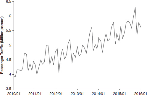
We focus on the monthly air travel demand for HKIA. Figure 6.1 shows the historical time series of the air passenger traffic in HKIA during the period of 2010 to 2015, and the historical data demonstrate a strong seasonality. In the following empirical analysis, the forecasting performance comparisons of various models are mainly based on two frequently used error measures: RMSE and MAPE, which were presented in Eq. (5.1) and Eq. (5.2).

6.2.2 Comparison results

The sample data in the period of years 2010 to 2014 are used for the model construction process, and then two approaches’ forecasting performance for the future 1- and 2-step, i.e., January and February in 2015, is compared. There are three models in total to be compared in this section. The first model is constructed with no CNY effect regressors. For the second model, we add several CNY effect regressors generated by the Genhol program, which represents a traditional and common approach as previously described. Note that the before-holiday effect (CNY_before) and the during-holiday effect (CNY_during) are both significant in our data, and note that the number in square brackets denotes the length of the predefined holiday intervals. Then for the third model, we add an exogenous variable constructed with the Google Trends data to capture the CNY effect. We tried several search key terms to get a good exogenous variable, and finally the Google Trends data of key term ‘Chinese new year’ were selected due to their good modeling performance. Besides the CNY effect regressors, the model selection process also chooses: 1) model orders for the SARIMA structure; 2) trading day effect (Leap Year); 3) Easter holiday effects (Easter); and 4) the outliers. The regression results and performance comparison results are shown in Table 6.1 and Table 6.2, respectively.

Figure 6.1 Historical air passenger traffic in HKIA

The comparison results in Table 6.2 show that the use of Google Trends data in model m3 can remarkably improve the forecasting performance for January and February. Thus, we can say that the use of Google Trends data is the best in quantifying the CNY effect. In the next section, we propose an air travel demand forecasting framework with the use of Google Trends data.

6.3 The proposed forecasting framework

The seasonal decomposition (SD)-based hybrid forecasting method has been proven to be a superior method in several demand forecasting studies. For example, Wang et al. (2011) proposed a SD-based LSSVR ensemble learning model for the Chinese hydropower consumption forecasting. Xie et al. (2014) confirmed the application of a SD-based forecasting method in the short-term air travel demand. However, there are two shortcomings in their methods. Firstly, neither of the studies considered the calendar effects when modeling the time series, which can have strong influence on special months such as the Januarys and Februarys. Secondly, they applied the LSSVR model, a nonlinear forecasting model, to model all components after the decomposition.

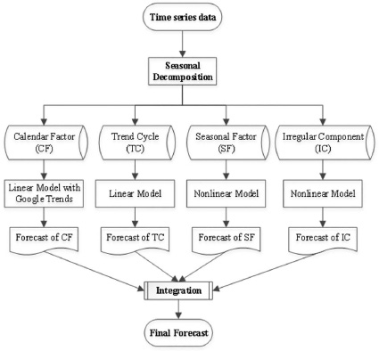
Hence, according to the principles of the TEI@I methodology, we propose a novel SD-based forecasting framework (Figure 6.2) in this section. The main aim is to provide a suitable forecasting method for the short-term air travel demand forecasting, especially for those special months that are influenced by the moving holiday effects.

6.3.1 Seasonal decomposition

In this chapter, we apply the X-13-ARIMA-SEATS program in most modeling processes. Firstly, we build a regARIMA model for the original time series y_t, to pre-adjust for the effects such as the outlier effects, the trading day effects and the holiday effects. We name the whole effect adjusted in the first step a calendar factor cf_t, in the following analysis. Secondly, the regression error of the regARIMA model, i.e., the pre-adjusted series y_t-cf_t, is typically decomposed into three components by the seasonal adjustment, namely trend cycle component tc_t, seasonal factor sf_t and irregular component ic_t. And an additive formulation is selected to integrate these four components, as follows:

Figure 6.2 The proposed SD-based forecasting framework

6.3.2 The overall forecasting process

The original time series is denoted as y_t(t = 1,2,...,T), and the forecasting horizon is defined as h, then according to our forecasting framework in Figure 6.2, the forecasts of y_t in the h step can be presented as follows:

There are three main steps contained in the proposed novel SD-based forecasting framework.

• Step 1: The original time series y_t is decomposed into four main components, cf_t, tc_t, sf_t and ic_t, through the X-13-ARIMA-SEATS program.
• Step 2: For each component obtained in the first step, the best single forecasting model is developed, where the calendar factor cf_t and trend cycle component tc_t are forecasted with linear models; and the seasonal factor sf_t and the irregular component ic_t are forecasted with the nonlinear models. Here, LSSVR models are constructed to forecast the sf_t and ic_t.
• Step 3: The h-step forecasts of cf_t, tc_t, sf_t and ic_t are integrated as a final forecast for the original time series according to Eq. (6.3).

6.3.3 Empirical analysis

In this section, the monthly air travel data shown in Figure 6.1 are used as a testing case to verify the effectiveness of our proposed forecasting framework. The sample data covering the period from January 2010 to December 2015 are separated into two subsets: the first 60 observations are taken as a training dataset; and the latter group of observations is taken as a testing dataset, to evaluate the short-term forecasting performance of our proposed forecasting framework, especially for January and February.

To further confirm the superior forecasting ability of our proposed forecasting framework, we also build several other popular forecasting models, including the SARIMA models, the LSSVR models and the hybrid forecasting method of Xie et al. (2014), where the original time series is first decomposed into three components, including the trend cycle component, seasonal factor and irregular component, respectively; then an LSSVR model is developed for each of the three components; a final forecast of the original time series is achieved by integrating all individual forecasts of the three components. This method of Xie et al. (2014) is named SD_LSSVR.

In this chapter, the X-13-ARIMA-SEATS program is adopted to implement seasonal decomposition with the R software package; and all SARIMA models are developed with the Eviews software package; while all LSSVR models are developed with the MATLAB software package. Table 6.3 lists the values of performance measurements MAPE and RMSE of different methods, for different forecasting time horizons. In addition, Figure 6.3 and Figure 6.4 show the forecasting performance comparison results visually.

From the comparison results of Table 6.3, it is clear that our proposed method is obviously outstanding in the short-term air travel demand, especially for January and February, which are greatly influenced by the CNY effects. We can draw several main conclusions as follows:

Firstly, these single models, including the SARIMA models and LSSVR models, perform poorly in this forecasting context. Possibly because there exist both the linear and nonlinear data patterns, and complex seasonal and calendar characteristics in the air travel demand time series, then a typical single linear model or a nonlinear model is not able to capture both patterns in the meantime. This result confirms our adoption of the decomposition-integration forecasting framework.

Secondly, as a SD-based forecasting method that does not consider the calendar effects, especially for the moving holiday effects, the SD_LSSVR model can achieve a better forecasting performance than those single models only in the 3-step’s and 6-step’s forecasting, while in the 1-step’s and 2-step’s forecasting, i.e., January and February, the forecasting error is not less than it is in single models. This reveals that the calendar effects can have significant influence on forecasting accuracy and should be modeled carefully. However, regardless of specific calendar effects, SD_LSSVR still performs more poorly than our proposed method in the 3-step’s and 6-step’s forecasting; this is mainly due to its adoption of the LSSVR models on the trend cycle component, ignoring the fact that linear pattern dominates in the trend cycle component and a linear model might be more proper.

Table 6.3 Forecasting performance comparison results

Figure 6.3 Performance comparison of different methods in terms of MAPE

Figure 6.4 Performance comparison of different methods in terms of RMSE

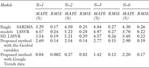
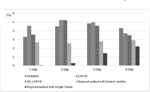
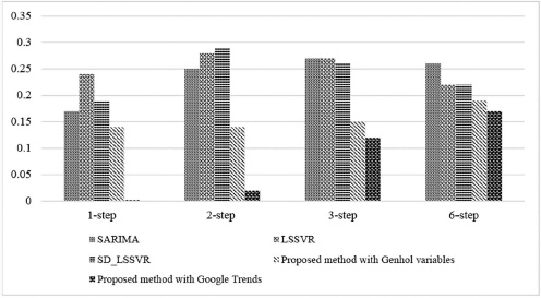
Finally, the forecasting performance of the proposed method with the Google Trends variables is significantly better compared to the model with Genhol variables, especially in 1-step and 2-step forecasting, i.e., for January and February. This confirms the superiority of using Google Trends data in quantifying the moving holiday effects.

6.4 Nowcasting

In this section, we will discuss and demonstrate the use of weekly Google Trends data for a nowcasting process. Many studies have discussed whether relevant intra-period information can help to forecast the target variable in the current period. This process is named ‘nowcasting’ in the literature (e.g., Nunes, 2005; Giannone et al., 2008). Nowcasting is especially important for making policy decisions in reality. Because in most cases the real economic data are released with a significant delay, the assessments of the current and future economic conditions can only be based on an incomplete dataset, thus making the assessment process difficult and inaccurate. Nowcasting has become a new release of data. And for the short-term demand forecasting, it is also meaningful to understand any information that is updated during the observation period and to explore this information’s value on improving the demand forecasting performance.

To prevent an unnecessary congestion or resource waste during the holiday periods, updated knowledge and information of the current state are especially important. As discussed previously, Google Trends data perform great in modeling the moving holiday effect. Hence, we will develop a proper model to incorporate the weekly Google Trends data that are available currently. The basic goal is to improve the forecasting accuracy of the holiday months, as new weekly information becomes available within the current month.

6.4.1 Methodology

The MIDAS models, representing the Mi(xed) Da(ta) S(ampling) models, were first introduced by Ghysels, Santa-Clara and Valkanov (2004). This model regresses the dependent variable on a distributed lag of independent variables which are sampled at a higher frequency. Compared to other methods that deal with mixed frequency problems, MIDAS models require parsimonious parameter specification and thus are computationally easier to implement.

(1) Basic MIDAS model

The basic MIDAS regression model with a single high-frequency explanatory variable and h-step ahead forecasting can be given as follows:

where the superscripts L and H denote low frequency/high frequency; u_t+h is the error term; ${\omega }_{N_H-j}\left({\theta }^H\right)$ is the weight function for the lagged high-frequency variables; and we assume that $\sum _{j=1}^{N_H-1}{\omega }_{N_H-j}\left({\theta }^H\right)\text{=}1$ to identify the slope coefficient β. The parameters $\left(\mu ,\beta ,{\theta }^H\right)$ are estimated by the nonlinear least squares method. Hence, a key feature of the MIDAS regression models is the utilization of a parsimonious and data-driven weighting scheme. Certainly, Eq. (6.4) can be extended to various model formulations, such as the DL-MIDAS, ARDL-MIDAS and GARCH-MIDAS, etc., according to specific data characteristics. In addition, there are various parameterizations of the weight scheme ${\omega }_{N_H-j}\left({\theta }^H\right)$ , which has been discussed comprehensively in Ghysels, Sinko and Valkanov (2007).

(2) MIDAS with leads

The nowcasting process can be implemented by specific MIDAS regression models with leads. In this section, the low-frequency variable is monthly air passenger traffic, and the high-frequency variable is weekly Google Trends data. Suppose now we are several weeks into month t+1, denoted as the number of leading weeks, $J_X^W$ , then we can achieve a basic MIDAS regression model with leads as follows:

where the superscripts M and W represent a monthly frequency and a weekly frequency, respectively. And a single weighting scheme is applied on the leads as well as the weekly lags. To account for other effects such as the autoregressive and exogenous effects, the final model formulation used in this study can be described as follows:

where $p_Y^M$ is the autoregressive order; E_i,t+1 denotes some exogenous variables that have a significant influence on the independent variable; and n_E is the number of exogenous variables. The parameters $\left(\mu ,{\mu }_{j+1},{\alpha }_i,\beta ,{\theta }^W\right)$ are to be estimated in Eq. (6.6).

6.4.2 Nowcasting results

Firstly, the forecasting performance for the holiday months, i.e., Januarys and Februarys, of the forecasting model with Genhol regressors and the nowcasting model in Eq. (6.6) is compared (see Table 6.4). Note that for the CNY effects, the forecasting model includes a CNY_before regressor and a CNY_during regressor generated from the Genhol program; for the nowcasting model, i.e., the MIDAS regression model with leads, Google Trends data are available several weeks ahead, and empirical results showed that models with Google Trends data of the first 2 weeks in the current month and the last week in the last month performed best. The results shown in Table 6.4 confirm that the nowcasting model with the weekly Google Trends data can improve the forecasting accuracy significantly in the current month.

Secondly, we then describe a nowcasting process for the future January 2016 in detail. The dataset of the period from January 2010 to December 2015 is used to estimate the parameters in Eq. (6.6). We are trying to nowcast the air travel demand in January 2016 with the two leading weeks’ Google Trends data in January 2016. The estimation process is implemented via the MIDAS MATLAB toolbox Version 2.0.

For model specification of Eq. (6.6), the calendar factor cf_t resulting from a SD process is taken as the independent monthly variable, and the weekly Google Trends data of key terms ‘Chinese new year’ are taken as a high-frequency explanatory weekly variable. Beyond that, we include an Easter holiday variable as an exogenous variable. The estimation results for Eq. (6.6) are described in Table 6.5. Except for the weekly explanatory variables, the regression model also includes a constant term (Constant), a three-order autoregressive term (Ylag3) and an exogenous variable for the Easter holiday effect (Easter). Also note that according to historical forecasting performance, i.e., MAPE and RMSE, and other criteria such as log likelihood and Akaike criteria, an Almon lag polynomial with order 2 is chosen as the weighting scheme for the high-frequency variables. The Almon lag polynomial specification of order P can be described as $\beta {\omega }_i\left({\theta }_0,\dots ,{\theta }_P\right)=\sum _{p=1}^P{\theta }_p{i}^p$ , where the parameters $\left({\theta }_0,\dots ,{\theta }_P\right)$ are to be estimated (denoted as AlmonDegree0, …, AlmonDegreeP in Table 6.5). Then $\beta {\omega }_i\left(\theta \right)$ in Eq. (6.6) can be estimated jointly.

The nowcasting value of calendar factor cf_t, achieved with estimated coefficient in Table 6.5, equals 0.1504. Then within our proposed framework in Figure 6.2, the values of trend cycle component tc_t, seasonal factor sf_t and irregular component ic_t in January 2016 are forecasted in the meantime. Finally, predicted values of the four components are integrated, equal to a demand forecast of about 5.615 million persons.

6.5 Conclusions

When implementing a short-term air travel demand forecasting with monthly or quarterly historical data, the seasonality is one of the most significant data patterns. Thus, it is natural to measure and adjust the seasonality in order to understand the underlying trends and then to achieve a good forecasting performance. Among all seasonal effects in the time series, the moving holiday effect is considered as the most difficult effect to quantify. In the literature of air travel demand forecasting research, seasonal adjustment is usually implemented by the popular methods such as the X-11 methods and the TRAMO/SEATS methods with the default settings, but few people have discussed the data-specific seasonal characteristics such as the moving holiday effects. Even though there are several built-in options provided in the existing programs to deal with the trading day effects and holiday effects such as the Easter holiday, Thanksgiving holiday, etc., a general method is still absent for managing the data-specific moving holiday effects. For example, the CNY holiday is the most important holiday in China and has great influence on almost every Chinese economic activity. However, the specific date of the Chinese New Year’s Day is moving year by year within the Gregorian calendar, which would lead to a misleading result applying the common seasonal adjustment method. Due to the strong influence on economic activities occurring in January and February, the CNY effect could result in a biased empirical finding if not modeled properly. In literature of the short-term Chinese air travel demand forecasting, we found that the forecasting errors for Januarys and Februarys are usually larger than for other months. This is mainly due to the moving holiday effects, i.e., the CNY effect, to a great extent.

Hence, modeling the moving holiday effects is one big problem that we should deal with in the first place when doing short-term air travel demand forecasting. Therefore, in this chapter, we proposed a seasonal decomposition-based forecasting framework with a novel use of Google Trends data, for modeling economic time series with complex seasonality patterns and especially to deal with the tough forecasting problem for those periods suffering moving holiday effects. The air passenger traffic of HKIA was taken as the historical data for an empirical analysis, where the CNY holiday effect was our main concern in this chapter. Firstly, we introduced two types of exogenous variables to capture the moving holiday effects based on either the holiday calendar or the Google Trends data, and then provided an empirical comparison for the two types of exogenous variables. The comparison results showed that constructing the exogenous variables with the Google Trends data, i.e., the users’ search data with proper key terms, is a better way to model the moving holiday effects. Secondly, we proposed a forecasting framework based on the seasonal decomposition method, with the novel use of Google Trends data as the exogenous variables to capture the moving holiday effects. In addition, we also presented a nowcasting process in detail with the weekly Google Trends data by adopting a MIDAS model with leads, to show that the information of a higher frequency in the current period can effectively help to improve the forecasting accuracy.

The empirical analysis was mainly focused on the Chinese New Year holiday, and the performance comparison results proved that the proposed method can not only solve the tough forecasting problem for those holiday periods, but also demonstrates superior forecasting performance in other forecasting time horizons. Firstly, to model specific moving holiday effects accurately, our proposed method can also be applied to other moving holiday effects in other types of economic time series. And another contribution of this chapter was that we presented a novel way to apply Google Trends data in the short-term air travel demand forecasting, which was a successful attempt and can be extended for other applications in the further research.

References

Bell, W. R., and Hillmer, S. C. (1984). Issues involved with the seasonal adjustment of economic time series. Journal of Business & Economic Statistics, 2(4), 291–320.
Choi, H., and Varian, H. (2012). Predicting the present with Google Trends. Economic Record, 88(s1), 2–9.
Ghysels, E., Santa-Clara, P., and Valkanov, R. (2004). The MIDAS Touch: Mixed Data Sampling Regression Models. Montreal, CIRANO.
Ghysels, E., Sinko, A., and Valkanov, R. (2007). MIDAS regressions: Further results and new directions. Econometric Reviews, 26(1), 53–90.
Giannone, D., Reichlin, L., and Small, D. (2008). Nowcasting: The real-time informational content of macroeconomic data. Journal of Monetary Economics, 55(4), 665–676.
Goel, S., Hofman, J. M., Lahaie, S., Pennock, D. M., and Watts, D. J. (2010). Predicting consumer behavior with Web search. Proceedings of the National Academy of Sciences, 107(41), 17486–17490.
Lin, J. L., and Liu, T. S. (2002). Modeling lunar calendar holiday effects in Taiwan. Taiwan Economic Forecast and Policy, 33(1), 1–37.
Nunes, L. C. (2005). Nowcasting quarterly GDP growth in a monthly coincident indicator model. Journal of Forecasting, 24(8), 575–592.
Wang, S., Yu, L., Tang, L., and Wang, S. (2011). A novel seasonal decomposition based least squares support vector regression ensemble learning approach for hydropower consumption forecasting in China. Energy, 36(11), 6542–6554.
Wu, L., and Brynjolfsson, E. (2015). The future of prediction: How Google searches foreshadow housing prices and sales. In: Goldfarb, A., Greenstein, S. M., and Tucker, C. E. (eds.), Economic Analysis of the Digital Economy. Chicago, University of Chicago Press, 89–118.
Xie, G., Wang, S., and Lai, K. K. (2014). Air Passenger Forecasting by Using a Hybrid Seasonal Decomposition and Least Squares Support Vector Regression Approach. DOI: http://2013.isiproceedings.org/Files/CPS205-P37-S.pdf