5   An integrated short-term forecasting framework with empirical mode decomposition method

In this chapter, we mainly focus on the model selection and construction of the short-term air travel demand framework, especially for the complex and volatile economic circumstances, where the common forecasting models such as the ARIMA models may fail with a relatively high probability. Thus, a novel and effective forecasting method is required. To achieve a better forecasting performance under complex and volatile economic circumstances, this chapter proposes an integrated short-term forecasting framework based on the TEI@I methodology, with the empirical mode decomposition method as a decomposition method. The final empirical results, based on historical air travel data of the Hong Kong International Airport, confirm the superior forecasting performance of our proposed method.

This chapter is organized as follows: section 5.1 briefly introduces the motivations of our proposal for a short-term air travel demand forecasting; section 5.2 describes the theoretical basis of the proposed forecasting method and the main implementation steps; then section 5.3 provides an empirical analysis for our method and section 5.4 concludes this chapter.

5.1 Introduction

Short-term air travel demand forecasting normally spans a forecasting time horizon of 1 to 12 months. And the short-term demand forecasts are often required in the management operations such as staffing, evaluating competitiveness and projecting equipment needs. For example, an airport might rely on the short-term forecast of total airport passenger arrivals as a key input for making daily operation decisions such as aircraft scheduling, maintenance planning, etc. Thus, forecasting accuracy is particularly important for reducing daily operation cost which could be huge when inappropriate decisions occur. Therefore, how to generate a good demand forecast becomes an inevitable challenge for both researchers and practitioners. Common methods and models for the short-term air travel demand forecasting include univariate time series models, AI-based forecasting models and multivariate regression models relying on macroeconomic variables such as GDP and population. The combination models of the aforementioned individual models are discussed and investigated widely in literature. Univariate time series models, such as the ARIMA models and the SARIMA models, are most popular mainly due to the low-cost implementation process and a good fitting effect. However, when the economic circumstance behaves with high uncertainty and volatility, the superiority of these traditional econometrical models becomes less evident. Hence, AI-based forecasting models, which exhibit great nonlinearity fitting performance, were developed to deal with this forecasting problem. Modeling nonlinearity is one main advantage of AI-based forecasting models. In addition to those univariate models, multivariate regression models with multiple macroeconomic variables can quantify the effects of other demand influencing factors and provide a better demand forecast when significant changes occur, but the main drawback of these models is the release delay of most macroeconomic variables, which could lead to the forecasts not being updated in time.

In fact, besides the periodic characteristics, the demand variation in a short-term future mainly results from the economic fluctuations and irregular events such as a financial crisis, earthquakes and terrorist attacks, etc. Consequently, under highly volatile and complex economic circumstances, demand forecasting becomes abnormally difficult. Common methods, including univariate time series models, multivariate causal-effect models and AI-based models which are all based on single structured historical data, seem not quite suitable under complex circumstances. Combination forecasting techniques have been discussed widely in literature and accepted by most researchers; see Timmermann (2006) for a comprehensive review. However, combining the individual models in an improper way cannot significantly improve the forecasting performance, or will even get a worse forecasting result. To deal with these challenges and obtain a higher forecasting accuracy, this chapter proposes an integrated short-term forecasting framework based on the TEI@I methodology (Wang, 2004). Therefore, one big contribution of this chapter is that we propose a novel combination method to the combination forecasting family, to face highly volatile circumstances. Then the Hong Kong International Airport is taken as an empirical case to test the superiority of our proposed framework. Empirical results show that the proposed method outperforms other competitive forecasting models, indicating that the proposed framework is a promising tool to forecast the short-term air travel demand, especially under volatile and complex economic circumstances.

5.2 The proposed forecasting framework

Under the volatile and complex economic circumstances, the air travel market would be strongly influenced by many irregular events (either natural or man-made) such as earthquakes, disease transmissions, terrorist attacks, etc., which will make the air travel demand particularly uncertain and fluctuating. Especially during some particular time periods, those irregular events are occurring more frequently. Under this type of background, the forecasting errors resulting from various traditional models will demonstrate a strong correlation. Hence, a traditional combination method, i.e., combining the forecasts of several individual models, cannot guarantee a better forecasting performance compared to that of those individual models.

Therefore, under volatile economic circumstances, it is far from easy to forecast the short-term air travel demand accurately due to the intrinsic complexity of its influencing factors. To deal with this difficult forecasting problem, we mainly employ the principle of ‘decompose, then assemble’, which is also called the ‘divide and conquer’ strategy in this chapter, to simplify a difficult forecasting task into several relatively easy subtasks. Considering the intrinsic complexity and nonlinearity in the historical data, the empirical mode decomposition (EMD) method is applied for a decomposition purpose. EMD, introduced by Huang et al. (1998), is to decompose original time series into several independent nearly periodic intrinsic modes. With the EMD method, any complex data can be decomposed into a finite number of components, to break down the original data. These nearly independent components can also be described as the intrinsic mode functions (IMFs). Since the EMD method can be applied to those nonlinear and nonstationary processes, it has been widely and successfully applied in the demand forecasting literature (e.g., Zhang et al., 2008; Wei and Chen, 2012; Chen et al., 2012). However, different from previous studies, the decomposition process in this chapter is implemented on the residual series of a linear forecasting model, instead of the original time series.

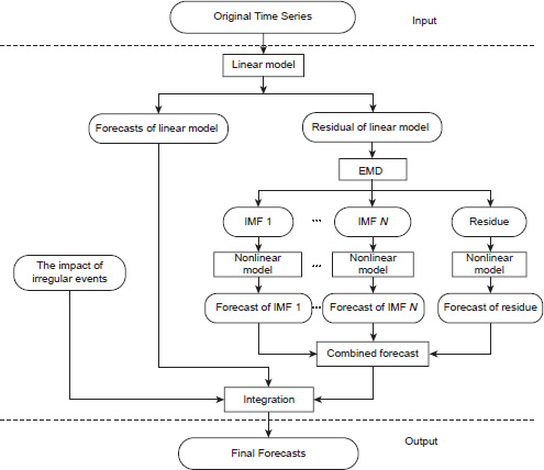
There are three main steps in our proposed integrated forecasting framework (see Figure 5.1). In the first step, the linear models are applied to modeling the original time series and capturing the linear component of the original time series; in the second step, the remaining nonlinear component, i.e., the residual component of the best linear model in the first step, is decomposed into several independent components with the EMD method, resulting in several IMFs and a residue, and suitable nonlinear models are constructed for every IMF and the residue. Then, all individual forecasts from those nonlinear models are combined to achieve a final forecast for the nonlinear components. Finally, in the third step, along with additive impact analysis of some irregular events with experts’ knowledge and experience, the best forecast of the linear component and the combined forecast of those nonlinear components are integrated into a final forecast. Within this proposed integrated air travel demand forecasting framework, the special part is that we only combine different forecasts for nonlinear components.

In the following empirical analysis, SARIMA models with several exogenous variables are selected as the linear model to forecast the linear component, while the LSSVR model is chosen as the nonlinear modeling technique. Denote the original time series by {y_t}, t = 1, 2,…,T. In terms of the general forecasting framework in Figure 5.1 and the previously introduced single techniques, a detailed implementation process of the proposed forecasting framework can be described as follows.

In the first step, adopt the SARIMA models to analyze the original time series {y_t}, and obtain the corresponding forecast ${\hat{y}}_t$ . Then in the meanwhile capture and extract the nonlinear component out of the original series y_t. In the second step, apply the EMD method to the residual series (i.e., $e_t=y_t-{\hat{y}}_t$ ) of the first step, where the residual series is considered as the remaining nonlinear component of the original series. As a result, we will achieve $e_t=im{f}_{t1}+im{f}_{t2}+\dots +im{f}_{tN}+residu{e}_t$ . Then with the application of LSSVR models on modeling every subcomponent, we will obtain a series of forecasts, denoted as ${\widehat{imf}}_1,{\widehat{imf}}_2,\dots {\widehat{imf}}_N,\widehat{residue}$ , respectively, and the overall forecast of e_t equals ${\hat{e}}_t={\widehat{imf}}_1\text{+}{\widehat{imf}}_2\text{+}\dots {\widehat{\text{+}imf}}_N\text{+}\widehat{residue}$ . This is the final forecast of the nonlinear component for the original time series. In the third step, according to the framework of the TEI@I methodology, along with experts’ knowledge and experience, judgmental adjustment is made when integrating all the aforementioned forecasting components, i.e., $y_f=f(y_t,e_t)$ , to obtain a final forecast of original time series. In order to verify the effectiveness of the proposed forecasting framework, air travel demand of Hong Kong International Airport is used as a case in the following empirical analysis.

Figure 5.1 General forecasting framework for short-term air travel demand

5.3 Empirical analysis

Hong Kong International Airport (HKIA) is a leading air passenger gateway and logistics hub in the Asia-Pacific region and also one of the world’s busiest airports in terms of international passenger and cargo movement. In the year 2015, HKIA served about 68.5 million passengers and handled 4.38 million tons of cargo, which made a significant economic contribution to the development of Hong Kong. According to the HKIA Authority, the airport is supporting the four pillar industries of Hong Kong’s economy, including the financial services industry, the trading and logistics industry, the tourism industry and the professional service industry. For years, the air transportation industry has played an important role in the development of the local economy, so it is necessary to provide more accurate demand forecasts for the future development and planning of HKIA.

5.3.1 Data description and evaluation criteria

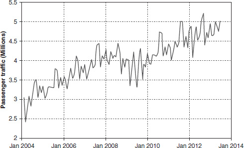
In this empirical analysis, the historical passenger movements of HKIA are used as the proxies for air travel demand. It is notable that we keep the data during the period from January 2004 to June 2013 instead of the latest data in our study. This is mainly because during the selected time window, the economic circumstances of the air transportation industry were very complex and volatile due to some unusual factors such as the snow disaster of the year 2008 in southern China, the SiChuan earthquake, the US subprime debit crisis and the European debit crisis, etc. It is valuable and suitable for testing the forecasting performance of our proposed forecasting framework under such a complex economic circumstance. The original data are downloaded from the CEIC macroeconomic database and are demonstrated in Figure 5.2. As Figure 5.2 shows, the historical passenger traffic in HKIA demonstrates a significant seasonality and some irregularity within this time window.

Figure 5.2 The monthly passenger traffic of HKIA

The sample data are divided into two subsets, i.e., the training subset and the testing subset. The training subset from January 2004 to December 2012 is used for the data modeling, and the remaining six observations from January 2013 to June 2013 are used for a model evaluation. Various individual forecasting models and different combination forecasting models are also generated in the meantime, to serve as the forecasting accuracy comparisons for the proposed forecasting framework. These accuracy comparisons are mainly based on the following two frequently used error measures, the Root Mean Squared Error (RMSE) and the Mean Absolute Percentage Error (MAPE), which are presented as follows:

where N is the number of observations in the testing dataset.

5.3.2 Modeling the linear component

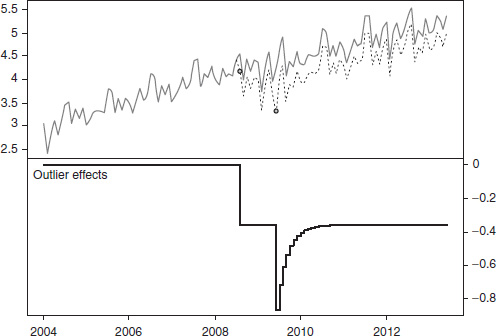
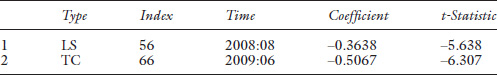
Figure 5.2 shows a strong seasonality and growth trend in the air travel demand of HKIA. However, there are also some outliers located in the historical time series. The effects of outliers are typically nonsystematic and should be specially quantified before modeling and forecasting, or the effects of those outliers may lead to a model misspecification, biased parameter estimation and poor forecasts with a large probability. Hence, before developing the SARIMA models, we firstly implement an automatic outlier detection procedure based on the approach described in Chen and Liu (1993) for time series with R package. The typical outlier types included in the detection procedure are Innovational Outliers (IO), Additive Outliers (AO), Level Shifts (LS) and Temporary Changes (TC), where for those TC outliers, the delta is setting as 0.5. Figure 5.3 shows the outlier detection results and the corresponding outlier effects, and Table 5.1 lists the detailed information about the detected outliers.

Based on the outlier detection results, a linear regression model that captures the outlier effects can be constructed as follows:

where u_t is the error term in Eq. (5.3); LS_t and TC_t are the effects of level shift outliers and temporary changes, respectively, and are constructed based on the results in Table 5.1, as follows:

Figure 5.3 The original series (dashed line) and the adjusted series (solid line) with corresponding outlier effects

Table 5.1 Outlier detection results

Then applying the SARIMA structure on the error term {u_t} and along with several common model selection criteria, we can develop a final linear model for the original series, as follows:

Eq. (5.4) is the final forecasting model for the linear component in our framework. Table 5.2 summarizes the estimation results of Eq. (5.4) in detail.

5.3.3 Modeling the nonlinear component

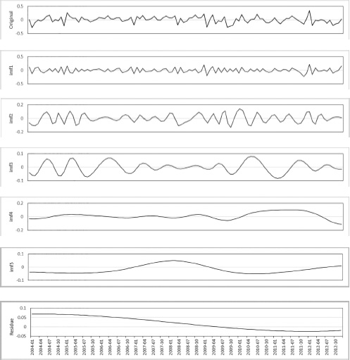
Through Eq. (5.4) and the estimation results in Table 5.2, we can obtain the nonlinear component of the original time series, i.e., the residual series $e_t=y_t-{\hat{y}}_t$ . The IMFs and residue are then derived by applying the EMD method to the residual series $e_t=y_t-{\hat{y}}_t$ , which are shown in Figure 5.4.

Then, the LSSVR models are constructed to fit the IMFs and residue in Figure 5.4, separately, and the forecasts derived from each of those LSSVR models are combined together into a final forecast of the nonlinear component $e_t=y_t-{\hat{y}}_t$ . Note that in the LSSVR modeling process, a Gaussian radial basis function is selected as the kernel function; and a grid search method is adopted to determine the optimal values of parameters to make the forecasting error in the training dataset smallest (Tay and Cao, 2001).

5.3.4 Model comparisons

Along with the experts’ judgmental adjustment, a final forecast of the future air travel demand is achieved by an integration of all forecasting results from the previous two forecasting steps. And we name our proposed forecasting model the ‘Partially-EMD’ model.

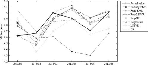
In the meanwhile, to confirm the superiority of our forecasting method compared to those traditional and common forecasting models, we build three popular single forecasting models including the linear regression model (regression), i.e., Eq. (5.4), LSSVR and GP. As for the GP models, we introduce the R square indicator as the measurement for identifying forecasting equations with a satisfactory goodness-of-fit for reproduction. We also build two popular combination forecasting models, named the Reg-LSSVR and Reg-GP, for a further comparison purpose on the same original time series, where the linear regression model Eq. (5.4) is applied for modeling the linear component and LSSVR or GP is applied for modeling the nonlinear component. Moreover, to confirm the effectiveness of our proposed method, we also build a ‘Fully-EMD’ forecasting model, where the EMD method is applied to the time series in Figure 5.2, and the LSSVR models are constructed for each component achieved from the EMD method, then the final forecast of a Fully-EMD forecasting model is achieved by combining all single forecasts from the last step. Figure 5.5 demonstrates the visual comparison of the actual value and forecasts from different forecasting models in this chapter. The forecasting performance comparisons of different models in terms of RMSE and MAPE are shown in Table 5.3.

Figure 5.4 The IMFs and residue for the nonlinear component

Figure 5.5 Forecasts of various methods

Table 5.3 Forecasting performance comparison

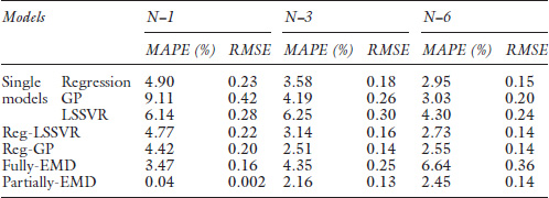
The empirical comparison results in Table 5.3 show that our proposed Partially-EMD method performs best in all forecasting time horizons in terms of both MAPE and RMSE. There are several conclusions as follows.

Firstly, comparing the forecasting performances of the three single forecasting models and the two popular combination forecasting models, we find that the Reg-LSSVR and Reg-GP models have effectively improved the forecasting accuracy. This result generally confirms that the common single models cannot perform very well under the volatile circumstances, mostly because the original time series contains both complex linear patterns and nonlinear patterns. Furthermore, the fact that our proposed Partially-EMD method performs better than the Reg-LSSVR and Reg-GP models confirms our assumptions, that is, under the volatile circumstances, the intrinsic and complex nonlinearity make the short-term forecasting exceptionally tough. Hence, for the nonlinear component, a single nonlinear forecasting model is not able to capture all characteristics. Thus, the EMD method applied for decomposing the nonlinear time series into several independent nearly periodic intrinsic modes is proven effective especially when dealing with a complex time series.

Secondly, the proposed Partially-EMD method significantly achieves a better forecasting performance than the Fully-EMD method, in terms of both MAPE and RMSE. These facts confirm the reasonableness of our proposed forecasting framework from another point of view. It is notable that the ‘partially combination’ strategy is more effective than the ‘fully combination’ strategy, mainly due to the dominance of the linearity in the time series of air passenger movement.

To sum up, the proposed forecasting model is significantly superior to all other forecasting models in terms of the forecasting accuracy, making it an effective model for short-term air travel demand forecasting under complex economic circumstances.

5.4 Conclusions

In a short-term future, besides the periodic factors, the variation of air travel demand mainly results from the economic fluctuations and irregular events such as a financial crisis, earthquakes and terrorist attacks, etc. And furthermore, under the highly volatile and complex economic circumstances, the irregular events will occur with a relatively high frequency. Consequently, the demand forecasting becomes abnormally difficult under volatile circumstances, and common forecasting methods, such as the univariate time series models, multivariate causal-effect models and AI-based models, seem not quite suitable in these situations. Hence, to deal with these challenges and obtain a higher forecasting accuracy, this chapter proposed an integrated short-term forecasting framework based on the TEI@I methodology. The integrated forecasting framework incorporates the empirical mode decomposition method in a partial way, to address the intrinsic complexity of air travel demand when the economic circumstances are unstable and uncertain. Specifically, the dominant linear trend in the original time series is captured and modeled by the linear models such as SARIMA models, and the corresponding residual series, considered as a nonlinear component for the original series, is firstly decomposed into several independent intrinsic mode functions and then each intrinsic mode function is modeled with an efficient nonlinear model such as the LSSVR model. The empirical comparison results, based on historical air travel data of the Hong Kong International Airport, show that this integrated forecasting framework can significantly improve the prediction performance.

In this chapter, we first briefly summarized the common forecasting models for the short-term air travel demand and introduced the motivations of our proposal for an integrated short-term air travel demand forecasting framework. Then based on the motivations, we proposed an integrated short-term air travel demand forecasting framework based on the TEI@I methodology, and described the main components and implementation steps in detail. Finally, we provided an empirical analysis for our proposed forecasting method with historical data of the Hong Kong International Airport, and the empirical results proved the superiority of our method, indicating that the proposed framework is a promising tool to forecast the short-term air travel demand, especially under volatile and complex economic circumstances. This is the first contribution of this chapter. The other big contribution is that we propose a novel combination method to the combination forecasting family, to face highly volatile circumstances.

It is notable that this framework is especially suitable for complex economic circumstances, where traditional forecasting models cannot achieve high forecasting performance. Under stable circumstances, traditional models like the SARIMA models are good enough to gain high forecasting accuracy, and the improvement by this forecasting framework will possibly be limited. Besides, this framework can also be applied to forecast other complex systems, such as container throughput forecasting, crude oil price forecasting, foreign trade volume forecasting, etc.

References

Chen, C. F., Lai, M. C., and Yeh, C. C. (2012). Forecasting tourism demand based on empirical mode decomposition and neural network. Knowledge-Based Systems, 26, 281–287.
Chen, C., and Liu, L. M. (1993). Joint estimation of model parameters and outlier effects in time series. Journal of the American Statistical Association, 88(421), 284–297.
Huang, N. E., Shen, Z., Long, S. R., Wu, M. C., Shih, H. H., Zheng, Q., Yen, N. C., Tung, C. C., and Liu, H. H. (1998). The empirical mode decomposition and the Hilbert spectrum for nonlinear and non-stationary time series analysis. Proceedings of the Royal Society of London A: Mathematical, Physical and Engineering Sciences, 454(1971), 903–995.
Tay, F. E. H., and Cao, L. (2001). Application of support vector machines in financial time series forecasting. Omega, 29(4), 309–317.
Timmermann, A. (2006). Forecast combinations. Handbook of Economic Forecasting, 1,135–196.
Wang, S. Y. (2004). TEI@I: A New Methodology for Studying Complex Systems. Proceedings of the International Workshop on Complexity Science, Tsukuba, Japan.
Wei, Y., and Chen, M. C. (2012). Forecasting the short-term metro passenger flow with empirical mode decomposition and neural networks. Transportation Research Part C: Emerging Technologies, 21(1), 148–162.
Zhang, X., Lai, K. K., and Wang, S. Y. (2008). A new approach for crude oil price analysis based on empirical mode decomposition. Energy Economics, 30(3), 905–918.