Search in book...
Toggle Font Controls
Create new playlist

Name your new playlist

Playlist description (optional)
Sign In

Email address

Password

Forgot Password?

or

Continue with Facebook

Continue with Google
Sign Up

Full Name

Email address

Confirm Email Address

Password

or

Continue with Facebook

Continue with Google

This chapter raises the research topic of unconstrained demand estimation and forecasting. Unconstrained demand forecasting is often difficult due to the unobservability of the applicable historical demand series. In this chapter, we propose a demand forecasting method based on the stochastic frontier analysis method and a model average technique. An empirical application of the medium-term air travel demand forecasting is implemented. The results of a forecasting performance comparison show that in addition to its ability to estimate unconstrained demand, our method outperforms other common forecasting methods in terms of forecasting passenger traffic.

The plan of this chapter is as follows: section 7.1 introduces the research backgrounds and motivations; section 7.2 describes our proposed demand forecasting methodology, and also introduces the stochastic frontier analysis method and the model average technique adopted in this methodology; section 7.3 presents an empirical application on the medium-term air travel demand forecasting and compares the proposed method with other common forecasting methods; section 7.4 concludes this chapter.

7.1 Introduction

Demand forecasting has long been investigated in related literature, and it is still a rapidly evolving research field. Researchers are now seeking to ‘exploit the availability of ever more plentiful data observations, greater computational power, and increasingly sophisticated economic and statistical theory’ (Clements and Hendry (Eds.), 2011). Common demand forecasting methods include statistical methods such as the linear multivariate regression models and univariate time series models (Cho, 2001; Goh and Law, 2002; Gil-Alana, 2005; Ediger and Akar, 2007), and artificial intelligence methods such as neural networks (Cho, 2003; Kon and Turner, 2005; Alekseev and Seixas, 2009) and support vector regression (Tay and Cao, 2001; Chen and Wang, 2007). Additionally, combination techniques are widely applied with the aforementioned models (Armstrong, 2001; Oh and Morzuch, 2005; Karlaftis, 2008; Xiao et al., 2014).

Conventionally, for demand modeling and forecasting purposes, the historical consumption quantities of a product or service are taken as proxies of the unobservable demands. However, the consumption quantity is usually not equal to the quantity that consumers actually demand. In addition to being led by demand, consumers’ behavior can be constrained by other factors, such as supply shortages and poor logistics service. These factors can be referred to as inefficiency of the producers. Unconstrained demand forecasting is an important issue, and methods for estimating unconstrained demand have been discussed mostly in hotel and airline revenue management (Weatherford and Kimes, 2003) by using either reservation denial data (Orkin, 1998) or various mathematical models (Wickham, 1995; Weatherford and Pölt, 2002). This chapter addresses the unconstrained demand forecasting problem, and in contrast to previous studies, we focus on demand at a more macro level, such as national demand. Although the existing forecasting methods have become more sophisticated and their forecasting accuracy has been markedly improved, the forecasting issue for this type of unconstrained demand is still ignored by most researchers.

The main purpose of this chapter is to develop a method that can estimate and forecast the unconstrained demand, i.e., the ‘true demand’, properly and scientifically. To achieve this goal, we propose a demand forecasting method based on stochastic frontier analysis (SFA) models and a model average technique. SFA is a parametric method that was developed to estimate efficient frontier and efficiency scores. It has been widely applied in efficiency assessment (e.g., Battese and Coelli, 1995; Jacobs R., 2001; Cullinane et al., 2006). The application of SFA in demand forecasting is one contribution of this chapter. Additionally, considering uncertainty in the selection of SFA models, cross-validation type model averaging is applied to improve the forecasting accuracy.

Model averaging, i.e., setting weights (which have values between 0 and 1, and sum to 1) to candidate models in some way, can prevent us from putting all of our inferential eggs in one unevenly woven basket (Longford, 2005). Model averaging often reduces the risk in regression estimation, as ‘betting’ on multiple models provides a type of insurance against a poor singly selected model (Leung and Barron, 2006). Bayesian model averaging (BMA) has long been a popular statistical technique; see Hoeting et al. (1999) for a comprehensive review. Recently, frequentist model averaging (FMA) has also been garnering interest; see, for example, Buckland et al. (1997), Hansen (2007), Zhang and Liang (2011) and Hansen and Racine (2012). In the current chapter, we follow the idea in Hansen and Racine (2012) and use cross-validation type model averaging to combine demand forecasts based on SFA models.

In the empirical application section, we aim to forecast Chinese air travel demand. To the best of our knowledge, all previous studies used historical passenger traffic as the proxy for travel demand and actually forecasted passenger traffic. However, by using our proposed method, we can estimate and forecast the unconstrained air travel demand based on historical passenger traffic data and several other demand explanatory variables.

7.2 Methodology

7.2.1 Stochastic frontier analysis models

The standard parametric SFA was proposed independently by Aigner et al. (1977) and Meeusen and van den Broeck (1977). The general setup is

y_{i} = x_{i}^{T} β - u_{i} + v_{i}, i = 1, \dots, n

$y_{i} = x_{i}^{T} β - u_{i} + v_{i}, i = 1, \dots, n$

(7.1)

where x is the exogenous explanatory variables vector, β is the coefficient vector, y_i is the response variable, u_i≥0 captures inefficiency of the producer and v_i captures outside influences beyond the control of the producer. It is assumed that u_i and v_i are independent of one other.

To estimate parameters in Eq. (7.1), some distribution assumptions on both u_i and v_i are often imposed. Then, all parameters in the model can be estimated using the maximum likelihood estimation method. Typically, v_i is assumed to be normally distributed with a mean 0 and variance $σ_{v}^{2}$ $σ_{v}^{2}$ , and the most common distributions for u_i are the truncated normal distribution $N^{+} (0, σ_{u}^{2})$ $N^{+} (0, σ_{u}^{2})$ and exponential distribution Exp(σ_u).

In the current study, we propose a demand forecasting method based on SFA models, using observable consumption quantities and demand explanatory variables. Following the general setup of the SFA model in Eq. (7.1), we assume that

\begin{array}{l} C_{i} = D_{i} - u_{i} \\ D_{i} = f (x_{i}) + v_{i} \end{array}

$\begin{array}{l} C_{i} = D_{i} - u_{i} \\ D_{i} = f (x_{i}) + v_{i} \end{array}$

(7.2)

where C_i denotes the actual consumption quantity, D_i denotes the unconstrained demand, f(x_i) is an unknown function and x_i contains exogenous explanatory variables that determine the demand. Thus, we have our proposed demand estimation SFA model as follows:

C_{i} = f (x_{i}) - u_{i} + v_{i}

$C_{i} = f (x_{i}) - u_{i} + v_{i}$

(7.3)

7.2.2 Model average

Assume that we have a total of S candidate SFA models and that the sth candidate model is

C_{i} = x_{(s), i}^{T} β_{(s),}_{i} - u_{(s), i} + v_{(s), i}

$C_{i} = x_{(s), i}^{T} β_{(s),}_{i} - u_{(s), i} + v_{(s), i}$

(7.4)

where $s \in {1, ..., S}$ $s \in {1, ..., S}$ . We use a simple linear function to approximate the unknown function f (x_i) in Eq. (7.2). Because it is uncertain which variables should be included in Eq. (7.4), we allow different variable combinations x_(s) to be used in different candidate models. For the sth candidate model, we assume $v_{(s), i} \sim N o r m a l_{(s)} (0, σ_{v, (s)}^{2})$ $v_{(s), i} \sim N o r m a l_{(s)} (0, σ_{v, (s)}^{2})$ and $u_{(s), i} \sim D_{(s)}^{+} (μ_{(s)}, σ_{u, (s)}^{2})$ $u_{(s), i} \sim D_{(s)}^{+} (μ_{(s)}, σ_{u, (s)}^{2})$ , using which we can calculate E(u_(s),i), which is denoted by $δ_{(s)} (μ_{(s)}, σ_{u, (s)})$ $δ_{(s)} (μ_{(s)}, σ_{u, (s)})$ . The distribution $D_{(s)}^{+}$ $D_{(s)}^{+}$ is chosen between the truncated normal and exponential distributions.

For the truncated normal distribution $D_{(s)}^{+} (μ_{(s)}, σ_{u, (s)}^{2}) = N o r m a l^{+} (μ, σ_{u}^{2})$ $D_{(s)}^{+} (μ_{(s)}, σ_{u, (s)}^{2}) = N o r m a l^{+} (μ, σ_{u}^{2})$ ,

δ_{(s)} (μ_{(s)}, σ_{u, (s)}) = μ_{(s)} + σ_{u, (s)} \frac{ϕ (μ_{(s)} / σ_{u, (s)})}{Φ (μ_{(s)} / σ_{u, (s)})}

$δ_{(s)} (μ_{(s)}, σ_{u, (s)}) = μ_{(s)} + σ_{u, (s)} \frac{ϕ (μ_{(s)} / σ_{u, (s)})}{Φ (μ_{(s)} / σ_{u, (s)})}$

(7.5)

For the exponential distribution $D_{(s)}^{+} (μ_{(s)}, σ_{u, (s)}^{2}) = \exp (σ_{u, (s)})$ $D_{(s)}^{+} (μ_{(s)}, σ_{u, (s)}^{2}) = \exp (σ_{u, (s)})$ ,

δ_{(s)} (μ_{(s)}, σ_{u, (s)}) = σ_{u, (s)}^{- 1}

$δ_{(s)} (μ_{(s)}, σ_{u, (s)}) = σ_{u, (s)}^{- 1}$

(7.6)

Under the sth candidate model, the unknown parameters β_(s), μ_(s), σ_u_,(s) and σ_v_,(s) can be estimated by maximum likelihood estimation. Let ${\hat{β}}_{(s)}$ ${\hat{β}}_{(s)}$ and ${\hat{σ}}_{v, (s)}$ ${\hat{σ}}_{v, (s)}$ be the maximum likelihood estimators of β_(s), μ_(s), σ_u_,(s) and σ_v_,(s), respectively. Then, for a new observation x_n₊₁, the forecast of demand is

{\hat{D}}_{n + 1, (s)} = x_{n + 1, (s)}^{T} {\hat{β}}_{(s)}

${\hat{D}}_{n + 1, (s)} = x_{n + 1, (s)}^{T} {\hat{β}}_{(s)}$

(7.7)

The forecast of consumption quantity is

{\hat{C}}_{n + 1, (s)} = {\hat{D}}_{n + 1, (s)} - δ_{(s)} ({\hat{μ}}_{(s)}, {\hat{σ}}_{u, (s)})

${\hat{C}}_{n + 1, (s)} = {\hat{D}}_{n + 1, (s)} - δ_{(s)} ({\hat{μ}}_{(s)}, {\hat{σ}}_{u, (s)})$

(7.8)

Write $w = {(w_{1}, \dots, w_{S})}^{T}$ $w = {(w_{1}, \dots, w_{S})}^{T}$ as the weight vector for model averaging, belonging to set $W = {w \in {[0, 1]}^{S} : \sum_{s = 1}^{S} w_{s} = 1}$ $W = {w \in {[0, 1]}^{S} : \sum_{s = 1}^{S} w_{s} = 1}$ . Then, the model average forecasts of demand and consumption quantity are as follows:

{\hat{D}}_{n + 1} (w) = \sum_{s = 1}^{S} w_{s} {\hat{D}}_{n + 1, (s)}

${\hat{D}}_{n + 1} (w) = \sum_{s = 1}^{S} w_{s} {\hat{D}}_{n + 1, (s)}$

(7.9)

{\hat{C}}_{n + 1} (w) = \sum_{s = 1}^{S} w_{s} {\hat{C}}_{n + 1, (s)}

${\hat{C}}_{n + 1} (w) = \sum_{s = 1}^{S} w_{s} {\hat{C}}_{n + 1, (s)}$

(7.10)

To choose the weight vector W in Eq. (7.9) and Eq. (7.10), we propose a cross-validation (CV) method as follows. Let

{\hat{D}}_{i, (s)} = x_{i, (s)}^{T} {\hat{β}}_{(s)}, {\hat{C}}_{i, (s)} = {\hat{D}}_{i, (s)} - δ_{(s)} ({\hat{μ}}_{(s)}, {\hat{σ}}_{u, (s)}), {\hat{D}}_{i} (w) = \sum_{s = 1}^{S} w_{s} {\hat{D}}_{i, (s)}, {\hat{C}}_{i} (w) = \sum_{s = 1}^{S} w_{s} {\hat{C}}_{i, (s)}

${\hat{D}}_{i, (s)} = x_{i, (s)}^{T} {\hat{β}}_{(s)}, {\hat{C}}_{i, (s)} = {\hat{D}}_{i, (s)} - δ_{(s)} ({\hat{μ}}_{(s)}, {\hat{σ}}_{u, (s)}), {\hat{D}}_{i} (w) = \sum_{s = 1}^{S} w_{s} {\hat{D}}_{i, (s)}, {\hat{C}}_{i} (w) = \sum_{s = 1}^{S} w_{s} {\hat{C}}_{i, (s)}$

and ${\hat{C}}_{i}^{(- i)} (w)$ ${\hat{C}}_{i}^{(- i)} (w)$ be the estimator of C_i without using the ith observation ${C_{i}, x_{i, (1)}, \dots, x_{i, (S)}}$ ${C_{i}, x_{i, (1)}, \dots, x_{i, (S)}}$ . Thus, our CV criterion is formulated as

C V (w) = \sum_{s = 1}^{S} {{\hat{C}}_{i}^{(- i)} (w) - C_{i}}^{2}

$C V (w) = \sum_{s = 1}^{S} {{\hat{C}}_{i}^{(- i)} (w) - C_{i}}^{2}$

(7.11)

The resulting weight vector is

_{w \in W} C V (w)

$_{w \in W} C V (w)$

(7.12)

The resulting model average forecasts for demand and consumption quantity are ${\hat{D}}_{n + 1} ()$ ${\hat{D}}_{n + 1} ()$ , respectively. It is straightforward to obtain that

\frac{1}{n} C V (w) \approx E {{\hat{C}}_{n + 1} (w) - C_{n + 1}}^{2}

$\frac{1}{n} C V (w) \approx E {{\hat{C}}_{n + 1} (w) - C_{n + 1}}^{2}$

(7.13)

Thus, by minimizing the CV criterion, the squared forecasting risk $E {{\hat{C}}_{n + 1} (w) - C_{n + 1}}^{2}$ $E {{\hat{C}}_{n + 1} (w) - C_{n + 1}}^{2}$ is also minimized approximately.

The following theorem shows that the squared forecasting risk is indeed minimized in a large sample. Let the squared forecasting risk functions of consumption and demand be, respectively,

r i s k_{C} (w) = E {{\hat{C}}_{n + 1} (w) - C_{n + 1}}^{2} and r i s k_{D} (w) = E {{\hat{D}}_{n + 1} (w) - D_{n + 1}}^{2}

$r i s k_{C} (w) = E {{\hat{C}}_{n + 1} (w) - C_{n + 1}}^{2} and r i s k_{D} (w) = E {{\hat{D}}_{n + 1} (w) - D_{n + 1}}^{2}$

Theorem 1. If Assumptions C.1–C.5 in Appendix A.1 are satisfied, then

\frac{r i s k_{C} ()}{\inf_{w \in W} r i s k_{C} (w)} \to 1

$\frac{r i s k_{C} ()}{\inf_{w \in W} r i s k_{C} (w)} \to 1$

(7.14)

in probability, as n → ∞. If Assumption C.6 in Appendix A.1 is further satisfied, then

\frac{r i s k_{D} ()}{\inf_{w \in W} r i s k_{D} (w)} \to 1

$\frac{r i s k_{D} ()}{\inf_{w \in W} r i s k_{D} (w)} \to 1$

(7.15)

in probability, as n → ∞.

Theorem 1 states that our model average consumption quantity and demand forecasts ${\hat{C}}_{n + 1} ()$ ${\hat{C}}_{n + 1} ()$ and ${\hat{D}}_{n + 1} ()$ ${\hat{D}}_{n + 1} ()$ are asymptotically identical to those obtained by using the infeasible best possible model average consumption quantity and demand forecasts, which means that our method is asymptotically optimal. The detailed assumptions and proof for Theorem 1 are given in Appendix A.2.

7.2.3 Demand forecasting processes

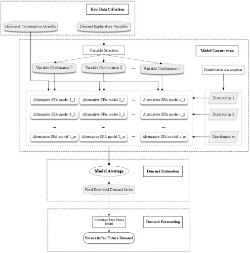
Figure 7.1 demonstrates our proposed demand forecasting framework based on SFA models and model averaging described in the previous section. There are four main steps in this method.

Step 1: Raw data collection. According to the experience of previous studies, the most important determinants and drivers that have a significant influence on demand are considered in the modeling process. Historical records of both consumption quantity and demand explanatory variables are collected.
Step 2: Model construction. Considering model uncertainty, a set of alternative SFA models with different combinations of explanatory variables and different distribution assumptions about u_i in Eq. (7.4) is constructed.
Step 3: Demand estimation. With model averaging, the average demand estimates are calculated based on the constructed SFA models from Step 2 and Eq. (7.9) and the final estimated demand series is generated.
Step 4: Demand forecasting. Finally, by using the average demand estimates as historical observations, the future demand forecasts can be achieved with standard forecasting models. In this study, a univariate time series model is applied to implement the future demand extrapolation.

Figure 7.1 Our proposed SFA-based demand forecasting framework

7.3 Empirical application

In this section, we provide an empirical application of our proposed demand forecasting method to air travel demand forecasting. The main objective is to forecast the air travel demand of Mainland China in the medium-term (3–5 years) future.

Hence, according to the framework shown in Figure 7.1, firstly, we select several explanatory variables for air travel demand modeling. Secondly, we construct all alternative SFA models with different explanatory variable combinations and two different distribution assumptions, i.e., truncated normal distribution and exponential distribution, of the inefficiency term in Eq. (7.4). Then, the unconstrained demand series is generated by a CV type model average technique. Finally, with the estimated demand series, future air travel demand forecasts are achieved with standard univariate time series models.

7.3.1 Data

For the application of our proposed framework, we use yearly passenger traffic of Mainland China as the dependent variable as well as several explanatory variables. All variables are defined and summarized in Table 7.1.

Table 7.1 Summary of variables
Variable	Definition	Category	Data source	Related studies
*Dependent variable*
Passenger traffic (P)	Yearly number of air passengers in Mainland China (million persons)		Civil Aviation Administration of China
*Explanatory variables*
Gross domestic product (GDP)	Yearly gross domestic product of China (billions of US dollars)	Economic factor	World Bank	e.g., Marazzo et al. (2010), Fernandes et al. (2010), Wang et al. (2010)
Trade value (TV)	Yearly total trade value of China (billions of US dollars)	Economic factor	UNCTAD STAT	e.g., Dargay and Hanly (2001), Abed et al. (2001)
Oil price (OP)	The price of crude oil (ten dollars per barrel)	Economic factor	WIND Database	e.g., Demirsoy (2012)
Urban population (UP)	Percentage of Chinese urban population to total population (%)	Demographic/social factor	World Bank	e.g., Lim (1997)

The yearly time series of historical data for Mainland China used in our analysis are during the period of years 1978 to 2014 (Figure 1.1). The figure shows a general tendency for sustained growth in the Chinese air transportation market. In the past decades, most of the yearly growth rate is located between 0 to 30 percent, and the average growth rate of the last 5 years is about 11.2 percent. In addition, Figure 7.2 shows the historical trends of all explanatory variables. In the subsequent modeling process, all value-related variables in Table 7.1 are recalculated in US dollars at constant prices (2005), to eliminate the inflation effects. All aggregative variables, i.e., gross domestic product and trade value, are used on a per capita basis, marked as GDP_pc and TV_pc, respectively.

In this study, we include the explanatory variable ‘urban population’, to replace the widely used ‘total population’ (e.g., Abed et al., 2001). In addition to reflecting the tendency of population size, ‘urban population’ can also reflect the nation’s urbanization degree, which has been proven to be a significant determinant of air travel demand. Table 7.2 lists the estimation results for these explanatory variables under a linear multivariate regression model.

Table 7.2 shows that all of the explanatory variables selected in this study are significant for explaining the dependent variable, i.e., passenger traffic. ‘GDP per capita’ and ‘trade value per capita’, as expected, have a positive influence on passenger traffic. These variables represent the level of economic activity and people’s living standards. In China’s present developing stage, people will fly relatively more often when their living standards are getting higher; the variable ‘urban population’, which represents the nation’s urbanization degree, is also proven to be a positive determinant for passenger traffic. In contrast, ‘oil price’, which is a proxy for traveling cost, is significantly negative, as expected.

Figure 7.2 Historical trends of explanatory variables

Table 7.2 The estimation results of a multiple regression model
Dependent variable: P *Sample period: 1978–2014*
Variable	Coefficient	Standard error	Prob.
GDP_pc	33.1520	4.2799	0.0000
TV_pc	7.1258	0.8736	0.0000
UP	0.3155	0.0964	0.0025
OP	–3.8260	0.5788	0.0000
R-squared	0.9949	Adjusted R-squared	0.9945

7.3.2 Method evaluation and comparison

To assess the forecasting performance of our proposed method, named MA-SFA by combining the abbreviations of model average (MA) and stochastic frontier analysis (SFA), we compare it with several other common methods in terms of their passenger traffic forecasting performance. According to the literature review, three widely applied methods, i.e., the linear multivariate regression model (Regression), autoregressive moving average (ARMA) model and back-propagation neural network (BPNN) algorithm, are constructed for performance comparison. The ARMA model and BPNN algorithm are applied on the single passenger traffic series, and the Regression model is built with all explanatory variables in Table 7.2. In this study, the Regression model and ARMA model are implemented in the Eviews software, and the BPNN and MA-SFA models are built in the MATLAB software. The original sample data are separated into two parts: the first 32 observations are used for model construction, and the remaining five observations are used for model evaluation.

The estimation results of the MA-SFA method are summarized in Table 7.3, where we list the top four SFA models according to the weights for each candidate SFA model. Note that with four explanatory variables and two distribution assumptions for u_i, we have $(C_{4}^{1} + C_{4}^{2} + C_{4}^{3} + C_{4}^{4}) \times 2 = 30$ $(C_{4}^{1} + C_{4}^{2} + C_{4}^{3} + C_{4}^{4}) \times 2 = 30$ candidate SFA models to calculate the average value, although most of them have lower weights than the SFA(4) model. Thus, in Table 7.3, we only list the top four for reference; the remaining models are available upon request.

Note that the distributions of u_i in those selected SFA models in Table 7.3 all happen to be truncated normal. Hence, the final average SFA model for air travel demand estimation, where the coefficients of each explanatory variable represent an average effect on air travel demand, can be described as follows:

\hat{P} = 26.6449 * G D P_p c + 8.0281 * T V_p c + 0.5027 * U P - 3.0543 * O P - 6 .3936

$\hat{P} = 26.6449 * G D P_p c + 8.0281 * T V_p c + 0.5027 * U P - 3.0543 * O P - 6 .3936$

(7.16)

Table 7.3 The main SFA models and corresponding estimated coefficients

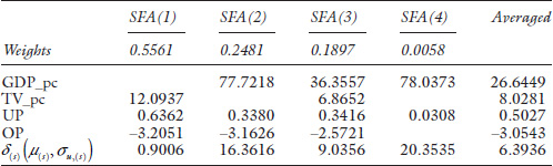
where 6.3936 is the average uncovered air travel demand in Mainland China, i.e., the inefficiency of the Chinese air travel market.

Eq. (7.16) shows the average effect of four key determinants on air travel demand. As expected, the GDP per capita and the trade value per capita have a positive influence on air travel demand. The estimated coefficient indicates that when the GDP per capita of China increases by one unit, the air travel demand will increase by approximately 26 units; when the percentage of urban population increases by one unit, the air travel demand will increase by approximately 0.5 of a unit. As expected, oil price, which is generally considered a proxy for passengers’ flying cost, has a negative impact on air travel demand. Our method does not provide standard errors for the estimated coefficients because it is very challenging, if not impossible, to study the distribution theory of our model average estimate.

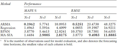
Figure 7.3 shows the actual passenger traffic, the air travel demand estimated by using our proposed MA-SFA method with sample data from the years 1978–2014 and the passenger traffic forecasts for the years 2010–2014 obtained from all four methods. The performance measures for various methods are also listed in Table 7.4.

From comparison results from both Table 7.4 and Figure 7.3, we can generally conclude that the forecasting performance of our proposed method is very promising. Several conclusions can be drawn from the aforementioned comparisons:

(a) In terms of both MAPE and RMSE, the MA-SFA method performs best in most forecasting time horizons, except for the 1-year forecast. These results suggest that although ARMA models are suitable for short-term forecasting, they tend to generate larger errors as the forecasting time horizons become longer. Thus, the proposed MA-SFA method is appropriate for medium-term demand forecasting, which is exactly the main forecasting objective in this empirical application.
(b) Compared to the ARMA and BPNN models, the multivariate models used in this study, i.e., the Regression model and MA-SFA method, perform better in longer forecasting time horizons, such as 5-year forecasting. The main reason for this difference is that the multivariate models consider the influence of other explanatory variables.
Figure 7.3 The actual passenger traffic and estimated demand series
Table 7.4 Performance comparison¹
(c) By comparing the forecasting performance of the MA-SFA method and the general multivariate linear regression method, there is a significant improvement in both MAPE and RMSE when applying the MA-SFA method. This result generally confirms the performance improvement that is observed when adopting the model average technique and SFA models.

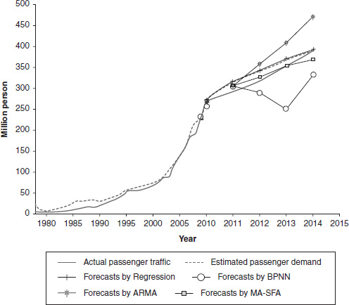
To sum up, on the one hand, the proposed method can estimate the unconstrained air travel demand (see Figure 7.3), which is the main contribution of this study; on the other hand, the proposed method also outperforms other commonly used models based on its performance in forecasting passenger traffic.

Finally, adopting standard ARIMA models for the estimated demand series, we forecast the Chinese air travel demand in 2017, 2018 and 2019 as 486.58, 529.50 and 578.11 million passengers, respectively.

7.4 Conclusions

In existing demand forecasting literature, the conventional way to quantify the unobservable demand is to take the actual consumption quantities as proxies for demands, which often leads to a substantial forecasting error. In this chapter, to overcome this problem, we proposed modeling demand by the SFA model. Also, a model average technique was developed to consider model uncertainty and to improve forecasting accuracy.

We further provided an empirical application on air travel demand forecasting. By our method, the underlying demand series was estimated with the historical passenger traffic and several explanatory variables of air travel demand. Then, an ARIMA model was applied on modeling the estimated demand series, to achieve the demand forecasts in future 3–5 years. Through the performance comparison with other commonly used methods, the performance of our methods was shown to be promising.

Lastly, we remark that this chapter proposed a general demand forecasting framework, which can also be applied in other industries for various forecasting time horizons.

References

Abed, S. Y., Ba-Fail, A. O., and Jasimuddin, S. M. (2001). An econometric analysis of international air travel demand in Saudi Arabia. Journal of Air Transport Management, 7(3), 143–148.

Aigner, D., Lovell, C. K., and Schmidt, P. (1977). Formulation and estimation of stochastic frontier production function models. Journal of Econometrics, 6(1), 21–37.

Alekseev, K. P. G., and Seixas, J. M. (2009). A multivariate neural forecasting modeling for air transport – preprocessed by decomposition: A Brazilian application. Journal of Air Transport Management, 15(5), 212–216.

Armstrong, J. S. (Ed.). (2001). Principles of Forecasting: A Handbook for Researchers and Practitioners. New York, Springer Science and Business Media.

Battese, G. E., and Coelli, T. J. (1995). A model for technical inefficiency effects in a stochastic frontier production function for panel data. Empirical Economics, 20(2), 325–332.

Buckland, S. T., Burnham, K. P., and Augustin, N. H. (1997). Model selection: An integral part of inference. Biometrics, 53(2), 603–618.

Chen, K. Y., and Wang, C. H. (2007). Support vector regression with genetic algorithms in forecasting tourism demand. Tourism Management, 28(1), 215–226.

Cho, V. (2001). Tourism forecasting and its relationship with leading economic indicators. Journal of Hospitality and Tourism Research, 25(4), 399–420.

Cho, V. (2003). A comparison of three different approaches to tourist arrival forecasting. Tourism Management, 24(3), 323–330.

Clements, M. P., and Hendry, D. F. (Eds.). (2011). The Oxford Handbook of Economic Forecasting. Oxford University Press, New York.

Cullinane, K., Wang, T. F., Song, D. W., and Ji, P. (2006). The technical efficiency of container ports: Comparing data envelopment analysis and stochastic frontier analysis. Transportation Research Part A: Policy and Practice, 40(4), 354–374.

Dargay, J., and Hanly, M. (2001). The determinants of the demand for international air travel to and from the UK. Proceedings of the 9th World Conference on Transport Research, Edinburgh, Scotland.

Demirsoy, C. (2012). Analysis of Stimulated Domestic Air Transport Demand in Turkey. Erasmus University Thesis Repository, Ankara, Turkey.

Ediger, V. Ş., and Akar, S. (2007). ARIMA forecasting of primary energy demand by fuel in Turkey. Energy Policy, 35(3), 1701–1708.

Fernandes, E., and Pacheco, R. R. (2010). The causal relationship between GDP and domestic air passenger traffic in Brazil. Transportation Planning and Technology, 33(7), 569–581.

Gil-Alana, L. A. (2005). Modelling international monthly arrivals using seasonal univariate long-memory processes. Tourism Management, 26(6), 867–878.

Goh, C., and Law, R. (2002). Modeling and forecasting tourism demand for arrivals with stochastic nonstationary seasonality and intervention. Tourism Management, 23(5), 499–510.

Hansen, B. E. (2007). Least squares model averaging. Econometrica, 75(4), 1175–1189.

Hansen, B. E., and Racine, J. S. (2012). Jackknife model averaging. Journal of Econometrics, 167(1), 38–46.

Hoeting, J. A., Madigan, D., Raftery, A. E., and Volinsky, C. T. (1999). Bayesian model averaging: A tutorial. Statistical Science, 14(4), 382–417.

Jacobs, R. (2001). Alternative methods to examine hospital efficiency: Data envelopment analysis and stochastic frontier analysis. Health Care Management Science, 4(2), 103–115.

Karlaftis, M. G. (2008). Demand forecasting in regional airports: dynamic Tobit models with GARCH errors. Sitraer, 7, 100–111.

Kon, S. C., and Turner, L. W. (2005). Neural network forecasting of tourism demand. Tourism Economics, 11(3), 301–328.

Leung, G., and Barron, A. R. (2006). Information theory and mixing least squares regressions. IEEE Transactions on Information Theory, 52(8), 3396–3410.

Lim, C. (1997). Review of international tourism demand models. Annals of Tourism Research, 24(4), 425–439.

Longford, N. T. (2005). Model selection and efficiency is ‘Which model… ?’ The right question? Journal of the Royal Statistical Society: Series A, 168(3), 469–472.

Marazzo, M., Scherre, R., and Fernandes, E. (2010). Air transport demand and economic growth in Brazil: A time series analysis. Transportation Research Part E: Logistics and Transportation Review, 46(2), 261–269.

Meeusen, W., and Van den Broeck, J. (1977). Efficiency estimation from Cobb-Douglas production functions with composed error. International Economic Review, 18(2), 435–444.

Oh, C. O., and Morzuch, B. J. (2005). Evaluating time-series models to forecast the demand for tourism in Singapore: Comparing within sample and post-sample results. Journal of Travel Research, 43(4), 404–413.

Orkin, E. B. (1998). Wishful thinking and rocket science: The essential matter of calculating unconstrained demand for revenue management. The Cornell Hotel and Restaurant Administration Quarterly, 39(4), 15–19.

Tay, F. E. H., and Cao, L. (2001). Application of support vector machines in financial time series forecasting. Omega, 29(4), 309–317.

Wang, S. J., Sui, D., and Hu, B. (2010). Forecasting technology of national-wide civil aviation traffic. Journal of Transportation Systems Engineering and Information Technology, 10(6), 95–102.

Weatherford, L. R., and Kimes, S. E. (2003). A comparison of forecasting methods for hotel revenue management. International Journal of Forecasting, 19(3), 401–415.

Weatherford, L. R., and Pölt, S. (2002). Better unconstraining of airline demand data in revenue management systems for improved forecast accuracy and greater revenues. Journal of Revenue and Pricing Management, 1(3), 234–254.

White, H. (1982). Maximum likelihood estimation of misspecified models. Econometrica: Journal of the Econometric Society, 50(1), 1–25.

Wickham, R. R. (1995). Evaluation of forecasting techniques for short-term demand of air transportation. Massachusetts Institute of Technology Thesis Repository, Cambridge, Massachusetts, US.

Xiao, Y., Liu, J. J., Hu, Y., Wang, Y., Lai, K. K., and Wang, S. (2014). A neuro-fuzzy combination model based on singular spectrum analysis for air transport demand forecasting. Journal of Air Transport Management, 39, 1–11.

Zhang, X., and Liang, H. (2011). Focused information criterion and model averaging for generalized additive partial linear models. Annals of Statistics, 39(1), 174–200.

..................Content has been hidden....................

You can't read the all page of ebook, please click here login for view all page.

Table of Contents for
7 A medium-term demand forecasting method based on stochastic frontier analysis and model average

7 A medium-term demand forecasting method based on stochastic frontier analysis and model average

7.1 Introduction

7.2 Methodology