8   Long-term air travel demand forecasting

An integrated method with ARDL bounds testing approach and scenario planning

The long-term air travel demand forecasting usually spans a period of 5 to 20 years and might be required in the management decisions such as facilities expansion or planning, long-term financial commitments, etc. Therefore, a long-term air travel demand forecast is of vital importance as a key basis for future infrastructure planning and construction decisions, especially for a fast-growing air transportation market like China. Scientific and effective planning can guarantee a sustainable development and prevent excess capacity. However, forecasting future demand over such a long time horizon is faced with challenges different from those in a short-term or medium-term forecasting. In this chapter, we propose an integrated long-term forecasting method for Chinese national air travel demand, based on the TEI@I methodology. The framework emphasizes the importance of experts’ domain knowledge in the demand forecasting process, especially for a long-term future.

This chapter is organized as follows: section 8.1 introduces the research backgrounds; section 8.2 presents our proposed integrated long-term demand forecasting method in detail; section 8.3 presents an empirical analysis with Chinese national air travel demand; finally section 8.4 concludes this chapter.

8.1 Introduction

Along with the process of economic globalization and urbanization, the Chinese air transportation industry has been experiencing a rapid and continuous growth in the past decades. In 2016, the air passenger traffic of China reached 487.9 million persons, which is almost 210 times that of the year 1978 and only surpassed by the United States. In the meantime, the sustainable growth of air travel demand also stimulates commercial airport construction in China. According to the planning of CAAC, the number of commercial airports will be more than 260 in the year 2020, to fulfill a future travel demand forecast of about 700 million persons. In addition, a modern airport system with wide airports coverage and a rational airports distribution will be built by the year 2025. At that time, there will be three world-class airport groups, 10 international transportation hubs and 29 regional transportation hubs in service, to support the development of the national economy and even the international economy. With the sustainable development of the national economy and the continuous improvement of people’s living standards, China has become one of the most promising air transportation markets in the world, and it is clear that the air transportation network has been considered as an indispensable engine of Chinese economic growth and become increasingly significant for the Chinese economy.

To support the growth of air travel demand and be wary of an excess capacity, an accurate long-term demand forecast is requisite. A long-term air travel forecast usually spans a period of 5 to 20 years and is often required in the management decisions such as facilities expansion or planning, long-term financial commitments, etc. The main objective of the long-term demand forecasting is to estimate the future air travel demand for a specific market with certain expected changes in the national economy and demography, or the development policy. Take IATA’s long-term traffic forecasting, for example; they use structural forecasting models calibrated largely on theory-derived parameters such as propensity to travel, which is linked to income.

However, forecasting future demand over such a long time horizon faces challenges different from those in the short-term or medium-term forecasting. Short-term data patterns will have little influence on the long-term behavior. The long-term forecasts rely greatly on researchers’ domain knowledge and opinion toward the target market and the assumed future value of some related variables such as economic growth. Hence, to fulfill such a complex job, a rigorous and mature forecasting methodology is the premise for satisfactory results.

From the literature, the most widely applied long-term forecasting methods often rely on multivariate econometric models, and implement trend extrapolation by assuming several alternative scenarios about the future. Specifically, for long-term air travel demand forecasting, Grubb and Mason (2001) applied Holt–Winters forecasting methods to a long time series of monthly air travel data since 1949. They believed that all variation was expressed in the historical data and the univariate methods might have some advantages over the multivariate models. Finally, three scenarios about future trends were set for the prediction. According to Samagaio and Wolters (2010), with respect to the long-term forecasts of air travel demand, there was no consensus on the ‘best’ forecasting model. They adopted a Holt–Winters forecasting model to capture the characteristics (i.e., trend and seasonality) for a monthly time series. And a smoothing factor was considered for possible future trends. Based on those two former studies, Scarpel (2013) proposed an integrated mixture of the local experts model to take advantage of both univariate methods and causal models. Scarpel stated that such an approach was suitable for rapidly changing situations, then following the study of Grubb and Mason (2001), he adopted three GDP growth scenarios for a 5-year forecast.

These studies all emphasized that the trend component was the most vital component for the air travel demand long-term forecasting, and then implemented a trend extrapolation basically relying on historical data and information. However, the assumption that the future will look like the past is usually not necessarily true in such a long-term future. The long-term forecasts also rely greatly on the researchers’ domain knowledge and opinion toward the target market. Hence, in this chapter, we propose an integrated method for long-term air travel demand forecasting in China, to extrapolate the main trend not only relying on our own historical information, but also learning the development experience from other developed markets, where experts’ knowledge plays a leading role in the main processes.

8.2 The proposed forecasting framework

Developing a sound demand forecasting framework is complex due to the uncertainty associated not only with the key explanatory variables’ value but also with the relationship between demand and its explanatory variables. In this chapter, we propose an integrated method for the long-term demand forecasting, which is composed of three core modules and relies on information from both the historical time series and experts’ knowledge. The proposed long-term demand forecasting framework is shown in Figure 8.1.

As Figure 8.1 shows, there are three core function modules in this forecasting framework, described as follows:

(1) Cointegration relationship

The ‘Cointegration relationship’ module is mainly aiming at seeking and quantifying the cointegration relationship between the air travel demand and its key explanatory variables. It is usually intuitive to associate the concept of cointegration when doing long-term demand forecasting because cointegration can represent the long-run equilibrium relationship to some extent.

(2) Long-term evolution pattern

The ‘Long-term evolution pattern’ module is mainly to explore and draw the possible future evolution patterns based on the development experience of other developed markets. The development experience of other developed markets usually has a great value of reference for China’s future development. In the common long-term demand forecasting methods, researchers seldom considered the reference information from other countries. This module is one of the highlights in our proposed long-term forecasting framework.

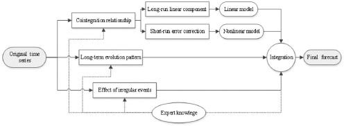
(3) Effect of irregular events

The ‘Effect of irregular events’ module is to analyze the effect of irregular events on air travel demand, and to judge if these effects are permanent or only transitory. The main objective of this module in the forecasting framework is to decide if there is any adjustment needed for our long-term forecasts.

Finally, by integrating all analysis results from each module, we can achieve a final long-term demand forecast. Note that the expert knowledge plays a vital role in almost every step in the forecasting framework. The corresponding methods and models involved in this study are described in detail next.

8.2.1 Cointegration relationship – the ARDL bounds testing approach

In the long-term demand forecasting literature, many studies have discussed the application of cointegration relationships in demand forecasting, and most of them adopted the traditional VEC framework of Engle and Granger (1987) to model the cointegration relationship. VEC models have a basic requirement that all variables should be an I(1) process, which is unsatisfied in many situations.

In this chapter, we apply the Autoregressive Distributed Lag (ARDL) bounds testing approach to investigate the cointegration relationship. Pesaran et al. (1999) presented that the ARDL model could also be applied to estimate the cointegration relationship, and proved that the estimated long-run and short-run parameters were unbiased and efficient. There are several advantages of the ARDL framework used for analyzing the cointegration relationship. Firstly, the variables involved can be either an I(0) or I(1) process, which loosens the strict assumptions when using the VEC models; secondly, an ARDL model does not require a symmetry of lag lengths for each variable, making it more proper for the small sample problems.

The original ARDL model can be written as follows:

$y_t={\alpha }_0+\sum _{i=1}^p{\gamma }_i{y}_{t-i}+\sum _{j=1}^k\sum _{i=0}^{q_j}{\beta }_{ji}{x}_{j,t-i}+{\epsilon }_t$

(8.1)

And the long-run equation can be written as follows:

$y_t\text{=}\alpha \text{+}\sum _{j=1}^k{\theta }_j{x}_{j,t}+u_t$

(8.2)

where, from Eq. (8.1) and Eq. (8.2), the estimated long-run coefficient is given by:

$\alpha =\frac{{\alpha }_0}{1-\sum _{i=1}^p{\gamma }_i}{\theta }_j=\frac{\sum _{i=1}^{q_j}{\beta }_{ji}}{1-\sum _{i=1}^p{\gamma }_i},u_t=\frac{{\epsilon }_t}{1-\sum _{i=1}^p{\gamma }_i}$

(8.3)

The cointegration regression form of an ARDL model, which is obtained by transforming Eq. (8.1) into the error correction (EC) form and substituting the long-run coefficients from Eq. (8.2), is written as follows:

$\Delta y_t=-\sum _{i=1}^{p-1}{\gamma }_i{}^{\text{*}}\Delta y_{t\text{-}1}\text{+}\sum _{j=1}^k\sum _{i=0}^{q_i-1}{\beta }_{ji}{}^{*}\Delta x_{j,t-i}-\hat{\varphi }E{C}_{t-1}+{\epsilon }_t$

(8.4)

where

The ARDL models are standard least square regressions which include lags of both the dependent variable and the explanatory variables as regressors. Although ARDL models have been used in econometrics literature for decades, they have gained popularity in recent years as a method of examining the long-run relationships and the cointegration relationships between variables.

8.2.2 Long-term evolution pattern – logistic growth model

The growth with saturation is frequently observed in the real world. This is economically natural due to the limited resources for a sustained growth. Logistic growth curves are widely and successfully applied to describe and forecast the evolution of these processes in research fields such as demographics, biology, economics, etc. (e.g., Berry et al., 1984; Bewley and Fiebig, 1988; To et al., 2012).

Many studies, such as Modis (2013) and Kwasnicki (2013), have presented the successful logistic curve fitting for the GDP growth. The growth of air travel demand is proven to be tightly related with the GDP growth. Therefore, in this chapter, we will fit the logistic growth curves on air passenger traffic of both China and several other developed air travel markets, trying to investigate and present some insights for the long-term air travel demand’s evolution patterns. The main purpose of a logistic growth model is to provide alternative long-term air travel demand forecasts with a trend analysis based on the well-known logistic curve theory.

The logistic growth model is described as follows:

$P{T}_t=\frac{K}{1+e^{-r(t-t_0)}}+C$

(8.5)

where PT_t denotes the passenger traffic in year t, K is the ceiling level of the logistic S-shaped pattern, r is the steepness of the logistic curve, t_o is the midpoint of the entire growth process and C is the eventual pedestal (positive or negative) on which the logistic may be sitting, often associated with missing early data. Thus, the growth curve is characterized by the four parameters $\left(K,r,t_0,C\right)$ . Let the estimators of those parameters be $\hat{K},\hat{r},{\hat{t}}_0,\hat{C}$ , respectively, then they are determined by minimizing the following objective function:

In this chapter, the curve fitting procedures are implemented with the MATLAB software package.

8.2.3 Effects of irregular events – Markov-switching regime approach

Macroeconomic variables are often affected by the unpredictable outside shocks which will create breaks in the time series immediately. In the past few decades, there have been several breaks in the Chinese air passenger traffic series. In general, these shocks correspond to some economic, financial and international events such as the economic recession or expansion, financial crises and political tensions, terrorist attacks, etc.

For the long-term demand forecasters and managers, it is an important question whether these exogenous shocks have a long-run influence on air travel demand or just a transitory effect. Njegovan (2006) discussed the question and dated the breaks through the sequential unit root testing approach, and the evidence for the United Kingdom, Germany and Australia showed that exogenous shocks to air passenger traffic were largely transitory. However, Njegovan’s approach can only date one break for the time series at one time.

Hence, to improve the performance of the breaks testing methods, in our proposed forecasting framework, we innovatively apply the Markov-switching (MS) regime approach to dating these break points, and this approach allows the users to date multiple breaks at one time. The MS regime model proposed by Hamilton (1989) is one of the most important structural change models in econometrics for several reasons. Firstly, the MS regime model allows for both changes in mean and variance; secondly, it also allows for multiple breaks dating, which is more proper in this context.

In general, a simple autoregressive model of order p with the M-state Markov-switching mean and variance may be written as

$y_t-{\mu }_{s_t}={\varphi }_1\left(y_{t-1}-{\mu }_{s_{t-1}}\right)+\cdots +{\varphi }_p\left(y_{t-p}-{\mu }_{s_{t-p}}\right)+{\epsilon }_t$

(8.6)

where ${\epsilon }_t\sim N\left(0,{\sigma }_{s_t}^2\right)$ and ${\mu }_{s_t}={\mu }_1{s}_{1t}+\cdots +{\mu }_M{s}_{Mt},{\sigma }_{s_t}^2={\sigma }_1^2{s}_{1t}+\cdots +{\sigma }_M^2{s}_{Mt}$ , and we have s_Mt=1 if s_t=M, and s_Mt=0, otherwise. The transition probability is $p\left[s_t=j|s_{t-1}=i\right]=p_{ij};i,j=1,2,\dots ,M;\sum _j{p}_{ij}=1$ .

8.2.4 Scenario planning

In addition to the aforementioned three core modules, we also incorporate the scenario planning technique into our long-term demand forecasting framework, to provide the assumptions for the future values of several explanatory variables. The systematic application of scenarios to picture possible futures generally began after World War II, and the US Department of Defense used it formally on military planning in the 1950s (Amer et al., 2013). In the 1960s, the scenario planning method was widely accepted in the fields such as social forecasting and public policy analysis. It has also been frequently adopted in the long-term demand forecasting literature. Scenarios, several alternative and reasonable assumptions for the plausible future, are able to explore the great complexities and uncertainties of the more distant future. It is reasonable to consider several scenarios when forecasting a long-term demand because the structure of future demand is of great uncertainty and highly likely to change.

There are also many international organizations applying the scenario planning technique in their long-term strategy analysis reports, including the latest versions of these organizations’ reports, such as International Energy Agency for world energy output, International Monetary Fund for world economic outlook, Intergovernmental Panel on Climate Change for climate change and United Nations for various reports about demography, etc.

Scenario planning has limited applications in the air transportation sector to date. It could become increasingly valuable for navigating major future challenges, and be used to develop a strategic vision for where air transportation would like to be in the future.

8.3 Empirical analysis

8.3.1 Data

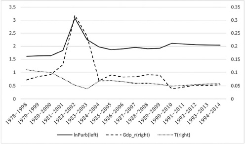
The availability of a consistent historical dataset allows the use of Chinese annual air passenger traffic for the period of the years 1978 to 2014 (Figure 1.1). Reviewing and gathering the previous studies that were already published on this demand forecasting subject has enabled us to make a list of possible explanatory variables, to develop the cointegration relationship of air travel demand with its influencing factors under the ARDL framework. Table 8.1 summarizes the brief definitions of all possible explanatory variables considered in the later modeling processes and their corresponding data sources. The data used in the model estimation process are collected from a variety of sources.

8.3.2 Cointegration relationship under ARDL framework

In this section, we develop the cointegration models through the ARDL bounds testing approach. Different combinations of possible explanatory variables listed in Table 8.1 have been constructed to develop the long-run relationships for air travel demand, then a model with the best forecasting performance has been selected out, where the MAPE is chosen as the performance criterion. All modeling processes are implemented through the Eviews 9.0 software. There are two main steps in the cointegration relationship modeling process.

Table 8.1 Summary of variables

Variable name	Definition	Unit	Source
Dependent variable
Passenger traffic (PT)	Yearly number of air passengers in Mainland China	Ten thousands	Civil Aviation Administration of China
Influencing factors
GDP per capita (Gpc)	Yearly GDP per capita of China	Current US dollars	World Bank
Trade value (Trade)	Total yearly value of exports and imports of China	Millions of US dollars	UNCTAD STAT
Population (Popu)	Total population of China	Ten thousands	National Bureau of Statistics of the People’s Republic of China
Oil price (OP)	The price of crude oil	Dollars per barrel	WIND Database
Total expenditure (Exp)	Yearly gross national expenditure	Billion dollars	World Bank
Growth of industry (Indu)	Annual growth of Chinese industry value added	%	World Bank
Population aged 15–64 (P15+)	Percentage of population aged 15–64 of Chinese total population	%	World Bank
Urban population (Purb)	Percentage of urban population of Chinese total population	%	World Bank
GDP growth rate (GDP_r)	Yearly growth rate of Chinese GDP	%	World Bank

Step 1: Unit root testing

The ARDL bounds testing approach to cointegration requires all regressors to be either an I(0) or I(1) process. Thus, the first step of modeling is the unit root testing. Table 8.2 presents the unit root test results for each possible variable included in the final model. The testing results show that all variables are either I(1) or I(0), which is satisfactory. Note that most of the variables in Table 8.1 have been logarithmically transformed for the following modeling.

Step 2: ARDL bounds testing approach to cointegration

Then, different combinations of explanatory variables are considered to develop long-run relationships for air travel demand. Through forecasting performance comparison results, the variables GDP growth rate (GDP_r), urban population percentage (lnPurb) and a time trend variable (T) are proven to be a powerful predictor combination, and a model with those three variables as the explanatory variables achieves the lowest MAPE value. In related literature, GDP growth rate has always been considered as the most important determinant for the air travel demand. However, in the context of the Chinese air travel market in its present stage, the rapid urbanization process and demographic advantage also play a vital role in the development of the air transportation industry.

After selecting the explanatory variables, we apply the rolling window technique to identify a proper estimation window for a future long-term forecast. Figure 8.2 shows that evolution path of the estimated coefficients for different estimation windows.

Finally, an estimation window of the period 1991–2011 with GDP growth rate (GDP_r), urban population percentage (lnPurb) and a time trend variable (T) as the explanatory variables is chosen to estimate the final coefficients. According to the bounds testing results in Table 8.3, the F-statistic is larger than any I1 Bound, which means that there is a significant long-run relationship existing between the logarithmic form of passenger traffic and the three explanatory variables.

Table 8.2 Summary of unit root test¹

Variable	Integration order	P-value
lnPT	I(1)	0.0066
lnTrade	I(1) with intercept	0.0002
lnPopu	I(0) with trend and intercept	0.0008
LnOP	I(1)	0.0000
lnGpc	I(1) with intercept	0.0126
lnExp	I(0) with intercept	0.0056
Indu	I(0) with intercept	0.0054
P15+	I(0) with trend and intercept	0.0172
GDP_r	I(0) with intercept	0.0044
lnPurb	I(1)	0.0867

Table 8.3 Bounds test for cointegration relationship

Null hypothesis: No long-run relationships exist
F-statistic	8.549190
Critical value bounds
Significance	I0 Bound	I1 Bound
10%	2.17	3.19
5%	2.72	3.83
2.5%	3.22	4.5
1%	3.88	5.3

The estimated model outlined next is based on minimizing the Schwarz Criterion. The derived long-run parameters, short-run parameters along with several diagnostic tests for the underlying ARDL model are reported in Table 8.4.

Thus, from equation CointEq=LNPT-(0.0459*GDP_r+2.0827*lnPurb+ 0.0517*T), we can get our final long-term forecasting equation as follows:

$\ln PT=0.0459*GDP\_r+2.0827*\ln Purb+0.0517*T+Co\mathrm{int}Eq$

(8.7)

where the forecasts of future GDP_r and lnPurb are setting with various scenarios; the error correction term CointEq is forecasted with the nonlinear models, e.g., least squares support vector regression models.

8.3.3 Logistic growth curve fitting

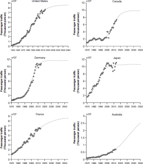
Figure 8.3 demonstrates the logistic growth fitting for six air travel markets, including the United States, Canada, Germany, Japan, France and Australia. These evolution patterns can be taken as the international experience references for the future’s evolution pattern of Chinese air travel demand. And the estimated parameters in Eq. (8.5) are listed in Table 8.5.

Table 8.4 ARDL model specifications

ARDL(1,0,0) is selected on Schwarz Criterion
Dependent variable: LnPT
21 observations used for estimation from 1991 to 2011
ARDL specifications
Regressors	Coefficient	Standard error	Prob.
LnPT(-1)	0.6049	0.1174	0.0001
GDP_r	0.0181	0.0072	0.0215
lnPurb	0.8229	0.2453	0.0038
T	0.0204	0.0076	0.0159
R-squared	0.9935	Schwarz Criterion	–2.2550
Log likelihood	29.7662	Durbin-Watson stat	2.1288
Long-run coefficients
Regressors	Coefficient	Standard error	Prob.
GDP_r	0.0459	0.0223	0.0557
LnPurb	2.0827	0.0899	0.0000
T	0.0517	0.0084	0.0000
Cointegration form
Regressors	Coefficient	Standard error	Prob.
D(GDP_r)	0.018117	0.0072	0.0215
D(lnPurb)	0.822859	0.2453	0.0038
D(T)	0.02041	0.0076	0.0159
CointEq(-1)	–0.3951	0.1174	0.0037
CointEq=LNPT-(0.0459*GDP_r+2.0827*lnPurb+0.0517*T)

The curve fitting results in Figure 8.3 show that except for Australia, all countries have passed through their midpoint, which is the inflection point of the logistic curve. And the curve of Japan has been 100 percent completed, followed by United States and Germany, which are nearly completed. In Japan, the air passenger traffic had already reached its ceiling in the beginning of the 21st century.

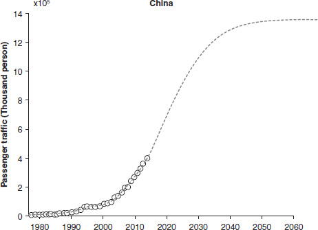
Figure 8.4 shows the fitting of the logistic curve on Chinese historical air passenger traffic. From the logistic point of view, the growth process of the air travel market in China is still in the very early stage, and can be expected to experience accelerating growth for several decades. According to the estimated parameters in Table 8.5, China will pass through its midpoint in the year 2021, and the passenger traffic for the years 2020 and 2030 is forecasted as 666,776 and 1,054,201 thousand persons, respectively.

The experience of other developed air travel markets can shed light on the general evolution and developing pattern of Chinese air travel demand. Due to the specific characteristics of an individual country, the results of logistic curve fitting can only be considered as a reference for long-term forecasting and further analysis is needed.

8.3.4 Effects of irregular events

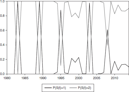
A two state Markov-switching regression model with the constant Markov transition probabilities for the difference form of LnPT, i.e., the growth rate of PT, is estimated. The transition probability is shown in Table 8.6, and the time path of smoothed probabilities for two regimes is shown in Figure 8.5.

The transition probabilities listed in Table 8.6 indicate that Regime 2 (i.e., S(t)=2) has the highest probability and duration. When the state is in Regime 1, it has the probability of almost 100 percent to transfer to Regime 2 (i.e., S(t)=1), which indicates that Regime 1 is an unsustainable or a transitory state. The time path of the smoothed probabilities demonstrated in Figure 8.5 has confirmed the same conclusion – that Regime 2 dominates almost all periods. As shown in Figure 8.5, the probabilities of Regime 1 are one or near one in the years 1983, 1989, 1995, 2003; and the probability of Regime 1 in year 2008 is larger than 0.6. From a historical point of view, these periods are just corresponding to several irregular events such as the second Gulf War and SARS in the year 2003, the 2007–2008 global financial crisis, etc. Hence, Figure 8.5 can be used to identify irregular events or shocks that have influenced the air travel market in China. From the results of both Table 8.6 and Figure 8.5, we can generally conclude that the effect of these irregular events on Chinese air travel demand is transitory and the air passenger traffic returns to its normal state following shocks, a conclusion similar to that reached in the study of Njegovan (2006).

Table 8.5 Estimated parameters of logistic curve fitting

	K	r	t0	C
United States	892912	0.0762	1987.477	–29220.997
China	1355409	0.1427	2020.244	841.594
Canada	84534	0.1802	2009.336	16712.280
Japan	86136	0.1850	1986.629	19095.322
France	93806	0.0644	1995.490	–6136.664
Germany	107245	0.2107	2000.613	10005.194
Australia	330050	0.0643	2035.125	3070.821

Table 8.6 Matrix of transition probability

	Regime 1	Regime 2	Duration	Probability
Regime 1	0.000008	0.999992	1.000008	0.1644
Regime 2	0.196809	0.803191	5.081066	0.8356

Hence, in long-term forecasting of the air travel demand, we can easily take on these irregular events and focus more on the underlying long-term trend.

8.3.5 Long-term demand forecasts with scenario planning

The long-term forecasts of air travel demand are obtained partly by implementing an out-of-sample forecasting of the estimated long-run Eq. (8.7). Then, one important step is to make several assumptions for the future values of those explanatory variables which have been identified in the long-run equilibration relationship. This is what the scenario planning does. The long-term air travel demand forecast presented next relies on crucial assumptions on two variables, and we set three assumptions for both of them.

For GDP growth, there are three assumptions as follows:

1. (a) ‘IMF GDP growth rate’ is based on the latest forecasts of GDP growth rates obtained from the IMF World Economic Outlook (WEO) Database.
2. (b) ‘Low GDP growth rates’, the IMF GDP growth rates projections, are decreased by 5 percent.
3. (c) ‘High GDP growth rates’, the IMF GDP growth rates projections, are increased by 5 percent.

For urban population percentage, there are three assumptions as follows:

1. (a) ‘UN urban population percentage’ is based on the annual percentage of population at mid-year residing in urban areas from the 2014 Revision of World Urbanization Prospects.
2. (b) ‘Low urban population percentage’, the UN projections of urban population percentage, is decreased by 5 percent.
3. (c) ‘High urban population percentage’, the UN projections of urban population percentage, is increased by 5 percent.

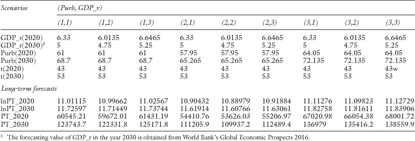
Then, we set (Purb, GDP_r) as a scenario. Thus with the assumptions for the GDP growth and urban population percentage, there are nine different scenarios in total. Table 8.7 lists the different long-term forecasts under the nine scenarios.

The driving effects of the GDP growth rate and urbanization population percentage on air travel demand can mainly be explained as three aspects. The first aspect can be summarized as the people’s living standards, which can mainly be reflected by the GDP growth rate. It is certain that a higher living standard results in more propensity and demand to fly. The other two aspects, named the demographical advantage and availability of air transportation mode, can both be reflected by the urban population percentage. The Chinese air transportation market is still in its early development stage, and we believe that those driving effects will still work in the following decades.

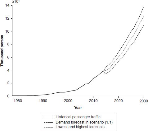
Finally, holding the forecasts of our long-run equation and the forecasts from logistic curve fitting, with the experts’ judgmental adjustment, we consider that the air travel demand in Mainland China will achieve about 600 to 660 million passengers in the year 2020; and will achieve 1.1 to 1.2 billion passengers in the year 2030, which is more conservative than IATA, who predicted that China will overtake the United States as the world’s largest passenger market by 2030. The long-term air travel demand forecasts are demonstrated in Figure 8.6.

8.4 Conclusions

Forecasting the future air travel demand over a time horizon longer than 5 years usually faces many challenges that have never been faced in the short-term or medium-term forecasting. The long-term forecasting relies much more on the researchers’ domain knowledge and opinions rather than the historical data and information. Hence, to fulfill such a complex job, a rigorous and mature forecasting methodology is the premise for satisfactory results. In the literature, the most widely applied long-term forecasting methods often rely on the historical time series, and implement a trend extrapolation with assumptions about several alternative scenarios about the future. These studies all emphasized that the trend component was the most vital component for a long-term demand, and then implemented a trend extrapolation basically relying on historical data and information. However, they usually missed the information of other markets’ developing experience, and the assumption that the future will look like the past is not necessarily true in such a long-term future.

Hence, in this chapter, we proposed an integrated method for long-term air travel demand forecasting in China mainly with an ARDL bounds testing approach to cointegration and scenario planning technique. This forecasting framework focuses on extrapolating the main trend not only relying on our own historical information, but also learning the development experience from other developed markets, where experts’ knowledge plays a leading role in the main processes. Using historical data of Chinese national air passenger traffic, we presented an empirical analysis to illustrate our proposed method. Within this forecasting framework, we can rely on not only China’s own development experience (i.e., the historical data pattern) by exploring the long-run relationship between demand and its drivers, but also learn the development experiences from other developed air travel markets with the logistic curve fitting technique.

Firstly, we introduced our proposed long-term forecasting framework in detail, and described the specific methods and models used in different modules, including the ARDL bound testing approach, the logistic growth model, the Markov-switching regime model and the scenario planning technique. Secondly, we implemented an empirical analysis with Chinese national air passenger time series. In the modeling of the long-run cointegration relationship, we found that the explanatory variables combination of GDP growth rate, urban population percentage and a time trend variable was proven to be a powerful predictor combination, and the model with those three variables as the explanatory variables achieved the lowest MAPE value. Then in the logistic curve fitting stage, the curve fitting results showed that except for Australia, all of the other five countries in this study have passed through the midpoint, and the curve of Japan has been 100 percent completed, followed by the United States and Germany, which are nearly completed. In Japan, the air passenger traffic had already reached its ceiling in the beginning of the 21st century. While in China, the growth process of the air travel market is still in the very early stage, and can be expected to experience accelerating growth for another several decades. In addition, we also adopted the Markov-switching regime models to date the break points for the air travel time series, and the results showed that the effect of these irregular shocks on Chinese air travel demand is transitory and the air passenger traffic returns to its normal state following shocks. Hence, in a long-term forecasting of the air travel demand, we can easily take on these irregular events and focus more on the underlying long-term trend. Finally, with several scenarios, we forecasted that the future air travel demand will be about 600 to 660 million passengers in the year 2020, and then will achieve 1.1 to 1.2 billion passengers in the year 2030.

It is worth noting that in this integrated forecasting framework, expert knowledge plays a leading role in almost every step. For example, expert knowledge also dominates the process of selecting proper explanatory variables for ARDL modeling. When we considered all possible variables in Table 8.1, variable population aged 15–64 was once proven to be a great predictor for air travel demand. However, later we found that the year 2015 will be an inflection point after which the percentage of population aged 15–64 will begin to drop. Combined with experts’ knowledge, we believe that a downward trend is not expected in the future Chinese air travel market. Hence, we excluded this variable even though it shows great forecasting performance.

One big contribution of this chapter is the general applicability of our proposed method, i.e., this forecasting method can also be applied to demand forecasting in other industries.

References

Amer, M., Daim, T. U., and Jetter, A. (2013). A review of scenario planning. Futures, 46, 23–40.
Berry, S. J., Coffey, D. S., Walsh, P. C., and Ewing, L. L. (1984). The development of human benign prostatic hyperplasia with age. The Journal of Urology, 132(3), 474–479.
Bewley, R., and Fiebig, D. G. (1988). A flexible logistic growth model with applications in telecommunications. International Journal of Forecasting, 4(2), 177–192.
Engle, R. F., and Granger, C. W. (1987). Co-integration and error correction: representation, estimation, and testing. Econometrica: Journal of the Econometric Society, 55(2), 251–276.
Grubb, H., and Mason, A. (2001). Long lead-time forecasting of UK air passengers by Holt-Winters methods with damped trend. International Journal of Forecasting, 17(1), 71–82.
Hamilton, J. D. (1989). A new approach to the economic analysis of nonstationary time series and the business cycle. Econometrica: Journal of the Econometric Society, 57(2), 357–384.
Kwasnicki, W. (2013). Logistic growth of the global economy and competitiveness of nations. Technological Forecasting and Social Change, 80(1), 50–76.
Modis, T. (2013). Long-term GDP forecasts and the prospects for growth. Technological Forecasting and Social Change, 80(8), 1557–1562.
Njegovan, N. (2006). Are shocks to air passenger traffic permanent or transitory? Implications for long-term air passenger forecasts for the UK. Journal of Transport Economics and Policy, 40(2), 315–328.
Pesaran, M. H., Shin, Y., and Smith, R. P. (1999). Pooled mean group estimation of dynamic heterogeneous panels. Journal of the American Statistical Association, 94(446), 621–634.
Samagaio, A., and Wolters, M. (2010). Comparative analysis of government forecasts for the Lisbon Airport. Journal of Air Transport Management, 16(4), 213–217.
Scarpel, R. A. (2013). Forecasting air passengers at São Paulo International Airport using a mixture of local experts model. Journal of Air Transport Management, 26, 35–39.
To, W. M., Lai, T. M., Lo, W. C., Lam, K. H., and Chung, W. L. (2012). The growth pattern and fuel life cycle analysis of the electricity consumption of Hong Kong. Environmental Pollution, 165, 1–10.