
12
Animation Systems
The majority of modern 3D games revolve around characters—often human or humanoid, sometimes animal or alien. Characters are unique because they need to move in a fluid, organic way. This poses a host of new technical challenges, over and above what is required to simulate and animate rigid objects like vehicles, projectiles, soccer balls and Tetris pieces. The task of imbuing characters with natural-looking motion is handled by an engine component known as the character animation system.
As we’ll see, an animation system gives game designers a powerful suite of tools that can be applied to non-characters as well as characters. Any game object that is not 100% rigid can take advantage of the animation system. So whenever you see a vehicle with moving parts, a piece of articulated machinery, trees waving gently in the breeze or even an exploding building in a game, chances are good that the object makes at least partial use of the game engine’s animation system.
12.1 Types of Character Animation
Character animation technology has come a long way since Donkey Kong. At first, games employed very simple techniques to provide the illusion of lifelike movement. As game hardware improved, more-advanced techniques became feasible in real time. Today, game designers have a host of powerful animation methods at their disposal. In this section, we’ll take a brief look at the evolution of character animation and outline the three most-common techniques used in modern game engines.
12.1.1 Cel Animation
The precursor to all game animation techniques is known as traditional animation, or hand-drawn animation. This is the technique used in the earliest animated cartoons. The illusion of motion is produced by displaying a sequence of still pictures known as frames in rapid succession. Real-time 3D rendering can be thought of as an electronic form of traditional animation, in that a sequence of still full-screen images is presented to the viewer over and over to produce the illusion of motion.
Cel animation is a specific type of traditional animation. A cel is a transparent sheet of plastic on which images can be painted or drawn. An animated sequence of cels can be placed on top of a fixed background painting or drawing to produce the illusion of motion without having to redraw the static background over and over.
The electronic equivalent to cel animation is a technology known as sprite animation. A sprite is a small bitmap that can be overlaid on top of a full-screen background image without disrupting it, often drawn with the aid of specialized graphics hardware. Hence, a sprite is to 2D game animation what a cel was to traditional animation. This technique was a staple during the 2D game era. Figure 12.1 shows the famous sequence of sprite bitmaps that were used to produce the illusion of a running humanoid character in almost every Mattel Intellivision game ever made. The sequence of frames was designed so that it animates smoothly even when it is repeated indefinitely—this is known as a looping animation. This particular animation would be called a run cycle in modern parlance, because it makes the character appear to be running. Characters typically have a number of looping animation cycles, including various idle cycles, a walk cycle and a run cycle.

12.1.2 Rigid Hierarchical Animation
Early 3D games like Doom continued to make use of a sprite-like animation system: Its monsters were nothing more than camera-facing quads, each of which displayed a sequence of texture bitmaps (known as an animated texture) to produce the illusion of motion. And this technique is still used today for low-resolution and/or distant objects—for example crowds in a stadium, or hordes of soldiers fighting a distant battle in the background. But for high-quality foreground characters, 3D graphics brought with it the need for improved character animation methods.
The earliest approach to 3D character animation is a technique known as rigid hierarchical animation. In this approach, a character is modeled as a collection of rigid pieces. A typical breakdown for a humanoid character might be pelvis, torso, upper arms, lower arms, upper legs, lower legs, hands, feet and head. The rigid pieces are constrained to one another in a hierarchical fashion, analogous to the manner in which a mammal’s bones are connected at the joints. This allows the character to move naturally. For example, when the upper arm is moved, the lower arm and hand will automatically follow it. A typical hierarchy has the pelvis at the root, with the torso and upper legs as its immediate children and so on as shown below:
Pelvis
 Torso
  UpperRightArm
    LowerRightArm
      RightHand
  UpperLeftArm
    UpperLeftArm
      LeftHand
  Head
 UpperRightLeg
  LowerRightLeg
    RightFoot
 UpperLeftLeg
  UpperLeftLeg
    LeftFoot
The big problem with the rigid hierarchy technique is that the behavior of the character’s body is often not very pleasing due to “cracking” at the joints. This is illustrated in Figure 12.2. Rigid hierarchical animation works well for robots and machinery that really are constructed of rigid parts, but it breaks down under scrutiny when applied to “fleshy” characters.
12.1.3 Per-Vertex Animation and Morph Targets
Rigid hierarchical animation tends to look unnatural because it is rigid. What we really want is a way to move individual vertices so that triangles can stretch to produce more natural-looking motion.
One way to achieve this is to apply a brute-force technique known as pervertex animation. In this approach, the vertices of the mesh are animated by an artist, and motion data is exported, which tells the game engine how to move each vertex at runtime. This technique can produce any mesh deformation imaginable (limited only by the tessellation of the surface). However, it is a data-intensive technique, since time-varying motion information must be stored for each vertex of the mesh. For this reason, it has little application to real-time games.
A variation on this technique known as morph target animation is used in some real-time games. In this approach, the vertices of a mesh are moved by an animator to create a relatively small set of fixed, extreme poses. Animations are produced by blending between two or more of these fixed poses at runtime. The position of each vertex is calculated using a simple linear interpolation (LERP) between the vertex’s positions in each of the extreme poses.
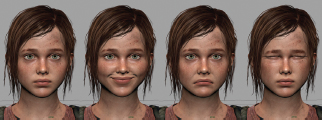
The morph target technique is often used for facial animation, because the human face is an extremely complex piece of anatomy, driven by roughly 50 muscles. Morph target animation gives an animator full control over every vertex of a facial mesh, allowing him or her to produce both subtle and extreme movements that approximate the musculature of the face well. Figure 12.3 shows a set of facial morph targets.
As computing power continues to increase, some studios are using jointed facial rigs containing hundreds of joints as an alternative to morph targets. Other studios combine the two techniques, using jointed rigs to achieve the primary pose of the face and then applying small tweaks via morph targets.

12.1.4 Skinned Animation
As the capabilities of game hardware improved further, an animation technology known as skinned animation was developed. This technique has many of the benefits of per-vertex and morph target animation—permitting the triangles of an animated mesh to deform. But it also enjoys the much more efficient performance and memory usage characteristics of rigid hierarchical animation. It is capable of producing reasonably realistic approximations to the movement of skin and clothing.
Skinned animation was first used by games like Super Mario 64, and it is still the most prevalent technique in use today, both by the game industry and the feature film industry. A host of famous modern game and movie characters, including the dinosaurs from Jurrassic Park, Solid Snake (Metal Gear Solid 4), Gollum (Lord of the Rings), Nathan Drake (Uncharted), Buzz Lightyear (Toy Story), Marcus Fenix (Gears of War) and Joel (The Last of Us) were all animated, in whole or in part, using skinned animation techniques. The remainder of this chapter will be devoted primarily to the study of skinned/skeletal animation.
In skinned animation, a skeleton is constructed from rigid “bones,” just as in rigid hierarchical animation. However, instead of rendering the rigid pieces on-screen, they remain hidden. A smooth continuous triangle mesh called a skin is bound to the joints of the skeleton; its vertices track the movements of the joints. Each vertex of the skin mesh can be weighted to multiple joints, so the skin can stretch in a natural way as the joints move.
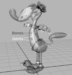
In Figure 12.4, we see Crank the Weasel, a game character designed by Eric Browning for Midway Home Entertainment in 2001. Crank’s outer skin is composed of a mesh of triangles, just like any other 3D model. However, inside him we can see the rigid bones and joints that make his skin move.
12.1.5 Animation Methods as Data Compression Techniques
The most flexible animation system conceivable would give the animator control over literally every infinitesimal point on an object’s surface. Of course, animating like this would result in an animation that contains a potentially infinite amount of data! Animating the vertices of a triangle mesh is a simplification of this ideal—in effect, we are compressing the amount of information needed to describe an animation by restricting ourselves to moving only the vertices. (Animating a set of control points is the analog of vertex animation for models constructed out of higher-order patches.) Morph targets can be thought of as an additional level of compression, achieved by imposing additional constraints on the system—vertices are constrained to move only along linear paths between a fixed number of predefined vertex positions. Skeletal animation is just another way to compress vertex animation data by imposing constraints. In this case, the motions of a relatively large number of vertices are constrained to follow the motions of a relatively small number of skeletal joints.
When considering the trade-offs between various animation techniques, it can be helpful to think of them as compression methods, analogous in many respects to video compression techniques. We should generally aim to select the animation method that provides the best compression without producing unacceptable visual artifacts. Skeletal animation provides the best compression when the motion of a single joint is magnified into the motions of many vertices. A character’s limbs act like rigid bodies for the most part, so they can be moved very efficiently with a skeleton. However, the motion of a face tends to be much more complex, with the motions of individual vertices being more independent. To convincingly animate a face using the skeletal approach, the required number of joints approaches the number of vertices in the mesh, thus diminishing its effectiveness as a compression technique. This is one reason why morph target techniques are often favored over the skeletal approach for facial animation. (Another common reason is that morph targets tend to be a more natural way for animators to work.)
12.2 Skeletons
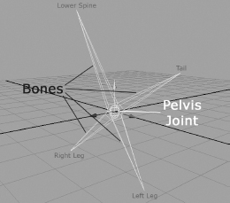
A skeleton is comprised of a hierarchy of rigid pieces known as joints. In the game industry, we often use the terms “joint” and “bone” interchangeably, but the term bone is actually a misnomer. Technically speaking, the joints are the objects that are directly manipulated by the animator, while the bones are simply the empty spaces between the joints. As an example, consider the pelvis joint in the Crank the Weasel character model. It is a single joint, but because it connects to four other joints (the tail, the spine and the left and right hip joints), this one joint appears to have four bones sticking out of it. This is shown in more detail in Figure 12.5. Game engines don’t care a whip about bones—only the joints matter. So whenever you hear the term “bone” being used in the industry, remember that 99% of the time we are actually speaking about joints.

12.2.1 The Skeleal Hierarchy
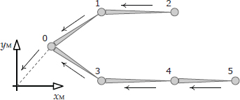
As we’ve mentioned, the joints in a skeleton form a hierarchy or tree structure. One joint is selected as the root, and all other joints are its children, grandchildren and so on. A typical joint hierarchy for skinned animation looks almost identical to a typical rigid hierarchy. For example, a humanoid character’s joint hierarchy might look something like the one depicted in Figure 12.6.
We usually assign each joint an index from 0 to N − 1. Because each joint has one and only one parent, the hierarchical structure of a skeleton can be fully described by storing the index of its parent with each joint. The root joint has no parent, so its parent index is usually set to an invalid value such as −1.
12.2.2 Representing a Skeleton in Memory
A skeleton is usually represented by a small top-level data structure that contains an array of data structures for the individual joints. The joints are usually listed in an order that ensures a child joint will always appear after its parent in the array. This implies that joint zero is always the root of the skeleton.
Joint indices are usually used to refer to joints within animation data structures. For example, a child joint typically refers to its parent joint by specifying its index. Likewise, in a skinned triangle mesh, a vertex refers to the joint or joints to which it is bound by index. This is much more efficient than referring to joints by name, both in terms of the amount of storage required (a joint index can be 8 bits wide, as long as we are willing to accept a maximum of 256 joints per skeleton) and in terms of the amount of time it takes to look up a referenced joint (we can use the joint index to jump immediately to a desired joint in the array).
Each joint data structure typically contains the following information:
A typical skeleton data structure might look something like this:
struct Joint
{
 Matrix4x3 m_invBindPose; // inverse bind pose
 // transform
const char* m_name;  // human-readable joint
 // name
 U8  m_iParent; // parent index or 0xFF
 // if root
};
struct Skeleton
{
 U32 m_jointCount; // number of joints
 Joint* m_aJoint;  // array of joints
};
12.3 Poses
No matter what technique is used to produce an animation, be it cel-based, rigid hierarchical or skinned/skeletal, every animation takes place over time. A character is imbued with the illusion of motion by arranging the character’s body into a sequence of discrete, still poses and then displaying those poses in rapid succession, usually at a rate of 30 or 60 poses per second. (Actually, as we’ll see in Section 12.4.1.1, we often interpolate between adjacent poses rather than displaying a single pose verbatim.) In skeletal animation, the pose of the skeleton directly controls the vertices of the mesh, and posing is the animator’s primary tool for breathing life into her characters. So clearly, before we can animate a skeleton, we must first understand how to pose it.
A skeleton is posed by rotating, translating and possibly scaling its joints in arbitrary ways. The pose of a joint is defined as the joint’s position, orientation and scale, relative to some frame of reference. A joint pose is usually represented by a 4 × 4 or 4 × 3 matrix, or by an SRT data structure (scale, quaternion rotation and vector translation). The pose of a skeleton is just the set of all of its joints’ poses and is normally represented as a simple array of matrices or SRTs.
12.3.1 Bind Pose
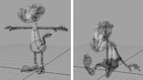
Two different poses of the same skeleton are shown in Figure 12.7. The pose on the left is a special pose known as the bind pose, also sometimes called the reference pose or the rest pose. This is the pose of the 3D mesh prior to being bound to the skeleton (hence the name). In other words, it is the pose that the mesh would assume if it were rendered as a regular, unskinned triangle mesh, without any skeleton at all. The bind pose is also called the T-pose because the character is usually standing with his feet slightly apart and his arms outstretched in the shape of the letter T. This particular stance is chosen because it keeps the limbs away from the body and each other, making the process of binding the vertices to the joints easier.
12.3.2 Local Poses
A joint’s pose is most often specified relative to its parent joint. A parent-relative pose allows a joint to move naturally. For example, if we rotate the shoulder joint, but leave the parent-relative poses of the elbow, wrist and fingers unchanged, the entire arm will rotate about the shoulder in a rigid manner, as we’d expect. We sometimes use the term local pose to describe a parent-relative pose. Local poses are almost always stored in SRT format, for reasons we’ll explore when we discuss animation blending.
Graphically, many 3D authoring packages like Maya represent joints as small spheres. However, a joint has a rotation and a scale, not just a translation, so this visualization can be a bit misleading. In fact, a joint actually defines a coordinate space no different in principle from the other spaces we’ve encountered (like model space, world space or view space). So it is best to picture a joint as a set of Cartesian coordinate axes. Maya gives the user the option of displaying a joint’s local coordinate axes—this is shown in Figure 12.8.
Mathematically, a joint pose is nothing more than an affine transformation. The pose of joint j can be written as the 4 × 4 affine transformation matrix Pj, which is comprised of a translation vector Tj, a 3 × 3 diagonal scale matrix Sj and a 3 × 3 rotation matrix Rj. The pose of an entire skeleton Pskel can be written as the set of all poses Pj, where j ranges from 0 to N − 1:

12.3.2.1 Joint Scale
Some game engines assume that joints will never be scaled, in which case Sj is simply omitted and assumed to be the identity matrix. Other engines make the assumption that scale will be uniform if present, meaning it is the same in all three dimensions. In this case, scale can be represented using a single scalar value sj. Some engines even permit nonuniform scale, in which case scale can be compactly represented by the three-element vector sj = [sjx sjy sjz]. The elements of the vector sj correspond to the three diagonal elements of the 3 × 3 scaling matrix Sj, so it is not really a vector per se. Game engines almost never permit shear, so Sj is almost never represented by a full 3 × 3 scale/shear matrix, although it certainly could be.
There are a number of benefits to omitting or constraining scale in a pose or animation. Clearly using a lower-dimensional scale representation can save memory. (Uniform scale requires a single floating-point scalar per joint per animation frame, while nonuniform scale requires three floats, and a full 3 × 3 scale-shear matrix requires nine.) Restricting our engine to uniform scale has the added benefit of ensuring that the bounding sphere of a joint will never be transformed into an ellipsoid, as it could be when scaled in a nonuniform manner. This greatly simplifies the mathematics of frustum and collision tests in engines that perform such tests on a per-joint basis.
12.3.2.2 Representing a Joint Pose in Memory
As we mentioned above, joint poses are usually stored in SRT format. In C++, such a data structure might look like this, where Q is first to ensure proper alignment and optimal structure packing. (Can you see why?)
struct JointPose
{
 Quaternion m_rot; // R
 Vector3  m_trans; // T
 F32   m_scale; // S (uniform scale only)
};
If nonuniform scale is permitted, we might define a joint pose like this instead:
struct JointPose
{
 Quaternion m_rot; // R
 Vector4  m_trans; // T
 Vector4  m_scale; // S
};
The local pose of an entire skeleton can be represented as follows, where it is understood that the array m_aLocalPose is dynamically allocated to contain just enough occurrences of JointPose to match the number of joints in the skeleton.
struct SkeletonPose
{
 Skeleton* m_pSkeleton; // skeleton + num joints
 JointPose* m_aLocalPose; // local joint poses
};
12.3.2.3 The Joint Pose as a Change of Basis
It’s important to remember that a local joint pose is specified relative to the joint’s immediate parent. Any affine transformation can be thought of as transforming points and vectors from one coordinate space to another. So when the joint pose transform Pj is applied to a point or vector that is expressed in the coordinate system of the joint j, the result is that same point or vector expressed in the space of the parent joint.
As we’ve done in earlier chapters, we’ll adopt the convention of using subscripts to denote the direction of a transformation. Since a joint pose takes points and vectors from the child joint’s space (C) to that of its parent joint (P), we can write it (PC→P)j. Alternatively, we can introduce the function p(j), which returns the parent index of joint j, and write the local pose of joint j as Pj→p(j).
On occasion we will need to transform points and vectors in the opposite direction—from parent space into the space of the child joint. This transformation is just the inverse of the local joint pose. Mathematically, Pp(j)→j = (Pj→p(j))−1.
12.3.3 Global Poses
Sometimes it is convenient to express a joint’s pose in model space or world space. This is called a global pose. Some engines express global poses in matrix form, while others use the SRT format.
Mathematically, the model-space pose of a joint (j → M) can be found by walking the skeletal hierarchy from the joint in question all the way to the root, multiplying the local poses (j → p(j)) as we go. Consider the hierarchy shown in Figure 12.9. The parent space of the root joint is defined to be model space, so p(0) ≡ M. The model-space pose of joint J2 can therefore be written as follows:
Likewise, the model-space pose of joint J5 is just
In general, the global pose (joint-to-model transform) of any joint j can be written as follows:
where it is understood that i becomes p(i) (the parent of joint i) after each iteration in the product, and p(0) ≡ M.
12.3.3.1 Representing a Global Pose in Memory
We can extend our SkeletonPose data structure to include the global pose as follows, where again we dynamically allocate the m_aGlobalPose array based on the number of joints in the skeleton:
struct SkeletonPose
{
 Skeleton* m_pSkeleton; // skeleton + num joints
 JointPose* m_aLocalPose; // local joint poses
 Matrix44* m_aGlobalPose; // global joint poses
};
12.4 Clips
In a film, every aspect of each scene is carefully planned out before any animations are created. This includes the movements of every character and prop in the scene, and even the movements of the camera. This means that an entire scene can be animated as one long, contiguous sequence of frames. And characters need not be animated at all whenever they are off-camera.
Game animation is different. A game is an interactive experience, so one cannot predict beforehand how the characters are going to move and behave. The player has full control over his or her character and usually has partial control over the camera as well. Even the decisions of the computer-driven non-player characters are strongly influenced by the unpredictable actions of the human player. As such, game animations are almost never created as long, contiguous sequences of frames. Instead, a game character’s movement must be broken down into a large number of fine-grained motions. We call these individual motions animation clips, or sometimes just animations.
Each clip causes the character to perform a single well-defined action. Some clips are designed to be looped—for example, a walk cycle or run cycle. Others are designed to be played once—for example, throwing an object or tripping and falling to the ground. Some clips affect the entire body of the character—the character jumping into the air for instance. Other clips affect only a part of the body—perhaps the character waving his right arm. The movements of any one game character are typically broken down into literally thousands of clips.
The only exception to this rule is when game characters are involved in a noninteractive portion of the game, known as an in-game cinematic (IGC), non-interactive sequence (NIS) or full-motion video (FMV). Noninteractive sequences are typically used to communicate story elements that do not lend themselves well to interactive gameplay, and they are created in much the same way computer-generated films are made (although they often make use of in-game assets like character meshes, skeletons and textures). The terms IGC and NIS typically refer to noninteractive sequences that are rendered in real time by the game engine itself. The term FMV applies to sequences that have been prerendered to an MP4, WMV or other type of movie file and are played back at runtime by the engine’s full-screen movie player.
A variation on this style of animation is a semi-interactive sequence known as a quick time event (QTE). In a QTE, the player must hit a button at the right moment during an otherwise noninteractive sequence in order to see the success animation and proceed; otherwise, a failure animation is played, and the player must try again, possibly losing a life or suffering some other consequence as a result.
12.4.1 The Local Timeline
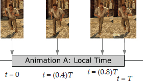
We can think of every animation clip as having a local timeline, usually denoted by the independent variable t. At the start of a clip, t = 0, and at the end, t = T, where T is the duration of the clip. Each unique value of the variable t is called a time index. An example of this is shown in Figure 12.10.
12.4.1.1 Pose Interpolation and Continuous Time
It’s important to realize that the rate at which frames are displayed to the viewer is not necessarily the same as the rate at which poses are created by the animator. In both film and game animation, the animator almost never poses the character every 1/30 or 1/60 of a second. Instead, the animator generates important poses known as key poses or key frames at specific times within the clip, and the computer calculates the poses in between via linear or curve-based interpolation. This is illustrated in Figure 12.11.
Because of the animation engine’s ability to interpolate poses (which we’ll explore in depth later in this chapter), we can actually sample the pose of the character at any time during the clip—not just on integer frame indices. In other words, an animation clip’s timeline is continuous. In computer animation, the time variable t is a real (floating-point) number, not an integer.
Film animation doesn’t take full advantage of the continuous nature of the animation timeline, because its frame rate is locked at exactly 24, 30 or 60 frames per second. In film, the viewer sees the characters’ poses at frames 1, 2, 3 and so on—there’s never any need to find a character’s pose on frame 3.7, for example. So in film animation, the animator doesn’t pay much (if any) attention to how the character looks in between the integral frame indices.
In contrast, a real-time game’s frame rate always varies a little, depending on how much load is currently being placed on the CPU and GPU. Also, game animations are sometimes time-scaled in order to make the character appear to move faster or slower than originally animated. So in a real-time game, an animation clip is almost never sampled on integer frame numbers. In theory, with a time scale of 1.0, a clip should be sampled at frames 1, 2, 3 and so on. But in practice, the player might actually see frames 1.1, 1.9, 3.2 and so on. And if the time scale is 0.5, then the player might actually see frames 1.1, 1.4, 1.9, 2.6, 3.2 and so on. A negative time scale can even be used to play an animation in reverse. So in game animation, time is both continuous and scalable.


12.4.1.2 Time Units
Because an animation’s timeline is continuous, time is best measured in units of seconds. Time can also be measured in units of frames, presuming we define the duration of a frame beforehand. Typical frame durations are 1/30 or 1/60 of a second for game animation. However, it’s important not to make the mistake of defining your time variable t as an integer that counts whole frames. No matter which time units are selected, t should be a real (floating-point) quantity, a fixed-point number or an integer that measures very small subframe time intervals. The goal is to have sufficient resolution in your time measurements for doing things like “tweening” between frames or scaling an animation’s playback speed.
12.4.1.3 Frame versus Sample
Unfortunately, the term frame has more than one common meaning in the game industry. This can lead to a great deal of confusion. Sometimes a frame is taken to be a period of time that is 1/30 or 1/60 of a second in duration. But in other contexts, the term frame is applied to a single point in time (e.g., we might speak of the pose of the character “at frame 42”).
I personally prefer to use the term sample to refer to a single point in time, and I reserve the word frame to describe a time period that is 1/30 or 1/60 of a second in duration. So for example, a one-second animation created at a rate of 30 frames per second would consist of 31 samples and would be 30 frames in duration, as shown in Figure 12.12. The term “sample” comes from the field of signal processing. A continuous-time signal (i.e., a function f(t)) can be converted into a set of discrete data points by sampling that signal at uniformly spaced time intervals. See Section 14.3.2.1 for more information on sampling.
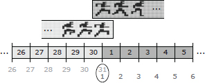
12.4.1.4 Frames, Samples and Looping Clips
When a clip is designed to be played over and over repeatedly, we say it is looped. If we imagine two copies of a 1 s (30-frame/31-sample) clip laid back-to-front, then sample 31 of the first clip will coincide exactly in time with sample 1 of the second clip, as shown in Figure 12.13. For a clip to loop properly, then, we can see that the pose of the character at the end of the clip must exactly match the pose at the beginning. This, in turn, implies that the last sample of a looping clip (in our example, sample 31) is redundant. Many game engines therefore omit the last sample of a looping clip.
This leads us to the following rules governing the number of samples and frames in any animation clip:
12.4.1.5 Normalized Time (Phase)
It is sometimes convenient to employ a normalized time unit u, such that u = 0 at the start of the animation, and u = 1 at the end, no matter what its duration T may be. We sometimes refer to normalized time as the phase of the animation clip, because u acts like the phase of a sine wave when the animation is looped. This is illustrated in Figure 12.14.
Normalized time is useful when synchronizing two or more animation clips that are not necessarily of the same absolute duration. For example, we might want to smoothly cross-fade from a 2-second (60-frame) run cycle into a 3-second (90-frame) walk cycle. To make the cross-fade look good, we want to ensure that the two animations remain synchronized at all times, so that the feet line up properly in both clips. We can accomplish this by simply setting the normalized start time of the walk clip, uwalk, to match the normalized time index of the run clip, urun. We then advance both clips at the same normalized rate so that they remain in sync. This is quite a bit easier and less error-prone than doing the synchronization using the absolute time indices twalk and trun.

12.4.2 The Global Timeline
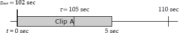
Just as every animation clip has a local timeline (whose clock starts at 0 at the beginning of the clip), every character in a game has a global timeline (whose clock starts when the character is first spawned into the game world, or perhaps at the start of the level or the entire game). In this book, we’ll use the time variable τ to measure global time, so as not to confuse it with the local time variable t.
We can think of playing an animation as simply mapping that clip’s local timeline onto the character’s global timeline. For example, Figure 12.15 illustrates playing animation clip A starting at a global time of τstart = 102 seconds.
As we saw above, playing a looping animation is like laying down an infinite number of back-to-front copies of the clip onto the global timeline. We can also imagine looping an animation a finite number of times, which corresponds to laying down a finite number of copies of the clip. This is illustrated in Figure 12.16.

Time-scaling a clip makes it appear to play back more quickly or more slowly than originally animated. To accomplish this, we simply scale the image of the clip when it is laid down onto the global timeline. Time-scaling is most naturally expressed as a playback rate, which we’ll denote R. For example, if an animation is to play back at twice the speed (R = 2), then we would scale the clip’s local timeline to one-half (1/R = 0.5) of its normal length when mapping it onto the global timeline. This is shown in Figure 12.17.
Playing a clip in reverse corresponds to using a time scale of −1, as shown in Figure 12.18.
In order to map an animation clip onto a global timeline, we need the following pieces of information about the clip:


Given this information, we can map from any global time τ to the corresponding local time t, and vice versa, using the following two relations:
If the animation doesn’t loop (N = 1), then we should clamp t into the valid range [0, T] before using it to sample a pose from the clip:
If the animation loops forever (N = ∞), then we bring t into the valid range by taking the remainder of the result after dividing by the duration T. This is accomplished via the modulo operator (mod, or % in C/C++), as shown below:
If the clip loops a finite number of times (1 < N < ∞), we must first clamp t into the range [0, NT] and then modulo that result by T in order to bring t into a valid range for sampling the clip:
Most game engines work directly with local animation timelines and don’t use the global timeline directly. However, working directly in terms of global times can have some incredibly useful benefits. For one thing, it makes synchronizing animations trivial.
12.4.3 Comparison of Local and Global Clocks
The animation system must keep track of the time indices of every animation that is currently playing. To do so, we have two choices:
The local clock approach has the benefit of being simple, and it is the most obvious choice when designing an animation system. However, the global clock approach has some distinct advantages, especially when it comes to synchronizing animations, either within the context of a single character or across multiple characters in a scene.
12.4.3.1 Synchronizing Animations with a Local Clock
With a local clock approach, we said that the origin of a clip’s local timeline (t = 0) is usually defined to coincide with the moment at which the clip starts playing. Thus, to synchronize two or more clips, they must be played at exactly the same moment in game time. This seems simple enough, but it can become quite tricky when the commands used to play the animations are coming from disparate engine subsystems.
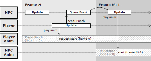
For example, let’s say we want to synchronize the player character’s punch animation with a non-player character’s corresponding hit reaction animation. The problem is that the player’s punch is initiated by the player subsystem in response to detecting that a button was hit on the joy pad. Meanwhile, the non-player character’s (NPC) hit reaction animation is played by the artificial intelligence (AI) subsystem. If the AI code runs before the player code in the game loop, there will be a one-frame delay between the start of the player’s punch and the start of the NPC’s reaction. And if the player code runs before the AI code, then the opposite problem occurs when an NPC tries to punch the player. If a message-passing (event) system is used to communicate between the two subsystems, additional delays might be incurred (see Section 16.8 for more details). This problem is illustrated in Figure 12.19.
void GameLoop()
{
 while (!quit)
 {
  // preliminary updates...
 UpdateAllNpcs(); // react to punch event
  // from last frame
 // more updates...
 UpdatePlayer(); // punch button hit - start punch
  // anim, and send event to NPC to
  // react
 // still more updates...
  }
}
12.4.3.2 Synchronizing Animations with a Global Clock
A global clock approach helps to alleviate many of these synchronization problems, because the origin of the timeline (τ = 0) is common across all clips by definition. If two or more animations’ global start times are numerically equal, the clips will start in perfect synchronization. If their playback rates are also equal, then they will remain in sync with no drift. It no longer matters when the code that plays each animation executes. Even if the AI code that plays the hit reaction ends up running a frame later than the player’s punch code, it is still trivial to keep the two clips in sync by simply noting the global start time of the punch and setting the global start time of the reaction animation to match it. This is shown in Figure 12.20.
Of course, we do need to ensure that the two characters’ global clocks match, but this is trivial to do. We can either adjust the global start times to take account of any differences in the characters’ clocks, or we can simply have all characters in the game share a single master clock.

12.4.4 A Simple Animation Data Format
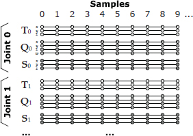
Typically, animation data is extracted from a Maya scene file by sampling the pose of the skeleton discretely at a rate of 30 or 60 samples per second. A sample comprises a full pose for each joint in the skeleton. The poses are usually stored in SRT format: For each joint j, the scale component is either a single floating-point scalar Sj or a three-element vector Sj = [Sjx Sjy Sjz]. The rotational component is of course a four-element quaternion Qj = [Qjx Qjy Qjz Qjw]. And the translational component is a three-element vector Tj = [Tjx Tjy Tjz]. We sometimes say that an animation consists of up to 10 channels per joint, in reference to the 10 components of Sj, Qj, and Tj. This is illustrated in Figure 12.21.
In C++, an animation clip can be represented in many different ways. Here is one possibility:
struct JointPose { … }; // SRT, defined as above
struct AnimationSample
{
 JointPose*  m_aJointPose; // array of joint
// poses
};
struct AnimationClip
{
  Skeleton* m_pSkeleton;
  F32  m_framesPerSecond;
  U32  m_frameCount;
  AnimationSample* m_aSamples; // array of samples
  bool  m_isLooping;
};
An animation clip is authored for a specific skeleton and generally won’t work on any other skeleton. As such, our example AnimationClip data structure contains a reference to its skeleton, m_pSkeleton. (In a real engine, this might be a unique skeleton id rather than a Skeleton* pointer. In this case, the engine would presumably provide a way to quickly and conveniently look up a skeleton by its unique id.)
The number of JointPoses in the m_aJointPose array within each sample is presumed to match the number of joints in the skeleton. The number of samples in the m_aSamples array is dictated by the frame count and by whether or not the clip is intended to loop. For a non-looping animation, the number of samples is (m_frameCount + 1). However, if the animation loops, then the last sample is identical to the first sample and is usually omitted. In this case, the sample count is equal to m_frameCount.
It’s important to realize that in a real game engine, animation data isn’t actually stored in this simplistic format. As we’ll see in Section 12.8, the data is usually compressed in various ways to save memory.
12.4.5 Continuous Channel Functions
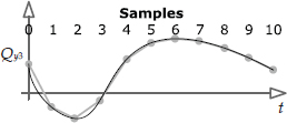
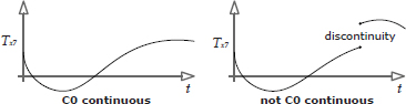
The samples of an animation clip are really just definitions of continuous functions over time. You can think of these as 10 scalar-valued functions of time per joint, or as two vector-valued functions and one quaternion-valued function per joint. Theoretically, these channel functions are smooth and continuous across the entire clip’s local timeline, as shown in Figure 12.22 (with the exception of explicitly authored discontinuities like camera cuts). In practice, however, many game engines interpolate linearly between the samples, in which case the functions actually used are piecewise linear approximations to the underlying continuous functions. This is depicted in Figure 12.23.
12.4.6 Metachannels
Many games permit additional “metachannels” of data to be defined for an animation. These channels can encode game-specific information that doesn’t have to do directly with posing the skeleton but which needs to be synchronized with the animation.
It is quite common to define a special channel that contains event triggers at various time indices, as shown in Figure 12.24. Whenever the animation’s local time index passes one of these triggers, an event is sent to the game engine, which can respond as it sees fit. (We’ll discuss events in detail in Chapter 16.) One common use of event triggers is to denote at which points during the animation certain sound or particle effects should be played. For example, when the left or right foot touches the ground, a footstep sound and a “cloud of dust” particle effect could be initiated.


Another common practice is to permit special joints, known in Maya as locators, to be animated along with the joints of the skeleton itself. Because a joint or locator is just an affine transform, these special joints can be used to encode the position and orientation of virtually any object in the game.
A typical application of animated locators is to specify how the game’s camera should be positioned and oriented during an animation. In Maya, a locator is constrained to a camera, and the camera is then animated along with the joints of the character(s) in the scene. The camera’s locator is exported and used in-game to move the game’s camera around during the animation. The field of view (focal length) of the camera, and possibly other camera attributes, can also be animated by placing the relevant data into one or more additional floating-point channels.
Other examples of non-joint animation channels include:
12.4.7 Relationship between Meshes, Skeletons and Clips
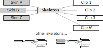
The UML diagram in Figure 12.25 shows how animation clip data interfaces with the skeletons, poses, meshes and other data in a game engine. Pay particular attention to the cardinality and direction of the relationships between these classes. The cardinality is shown just beside the tip or tail of the relationship arrow between classes—a one represents a single instance of the class, while an asterisk indicates many instances. For any one type of character, there will be one skeleton, one or more meshes and one or more animation clips. The skeleton is the central unifying element—the skins are attached to the skeleton but don’t have any relationship with the animation clips. Likewise, the clips are targeted at a particular skeleton, but they have no “knowledge” of the skin meshes. Figure 12.26 illustrates these relationships.
Game designers often try to reduce the number of unique skeletons in the game to a minimum, because each new skeleton generally requires a whole new set of animation clips. To provide the illusion of many different types of characters, it is usually better to create multiple meshes skinned to the same skeleton when possible, so that all of the characters can share a single set of animations.
12.4.7.1 Animation Retargeting
We said above that an animation is typically only compatible with a single skeleton. This limitation can be overcome via animation retargeting techniques.
Retargeting means using an animation authored for one skeleton to animate a different skeleton. If the two skeletons are morphologically identical, retargeting may boil down to a simple matter of joint index remapping. But when the two skeletons don’t match exactly, the retargeting problem becomes more complex. At Naughty Dog, the animators define a special pose known as the retarget pose. This pose captures the essential differences between the bind poses of the source and target skeletons, allowing the runtime retargeting system to adjust source poses so they will work more naturally on the target character.
Other more-advanced techniques exist for retargeting animations authored for one skeleton so that they work on a different skeleton. For more information, see “Feature Points Based Facial Animation Retargeting” by Ludovic Dutreve et al. (https://bit.ly/2HL9Cdr) and “Real-time Motion Retargeting to Highly Varied User-Created Morphologies” by Chris Hecker et al. (https://bit.ly/2vviG3x).

12.5 Skinning and Matrix Palette Generation
We’ve seen how to pose a skeleton by rotating, translating and possibly scaling its joints. And we know that any skeletal pose can be represented mathematically as a set of local (Pj→p(j)) or global (Pj→M) joint pose transformations, one for each joint j. Next, we will explore the process of attaching the vertices of a 3D mesh to a posed skeleton. This process is known as skinning.
12.5.1 Per-Vertex Skinning Information
A skinned mesh is attached to a skeleton by means of its vertices. Each vertex can be bound to one or more joints. If bound to a single joint, the vertex tracks that joint’s movement exactly. If bound to two or more joints, the vertex’s position becomes a weighted average of the positions it would have assumed had it been bound to each joint independently.
To skin a mesh to a skeleton, a 3D artist must supply the following additional information at each vertex:
The weighting factors are assumed to add to one, as is customary when calculating any weighted average.
Usually a game engine imposes an upper limit on the number of joints to which a single vertex can be bound. A four-joint limit is typical for a number of reasons. First, four 8-bit joint indices can be packed into a 32-bit word, which is convenient. Also, while it’s pretty easy to see a difference in quality between a two-, three- and even a four-joint-per-vertex model, most people cannot see a quality difference as the number of joints per vertex is increased beyond four.
Because the joint weights must sum to one, the last weight can be omitted and often is. (It can be calculated at runtime as w3 = 1 − (w0 + w1 + w2).) As such, a typical skinned vertex data structure might look as follows:
struct SkinnedVertex
{
 float m_position[3]; // (Px, Py, Pz)
 float m_normal[3];  // (Nx, Ny, Nz)
 float m_u, m_v;   // texture coords (u,v)
 U8  m_jointIndex[4]; // joint indices
 float m_jointWeight[3]; // joint weights (last
// weight omitted)
};
12.5.2 The Mathematics of Skinning
The vertices of a skinned mesh track the movements of the joint(s) to which they are bound. To make this happen mathematically, we would like to find a matrix that can transform the vertices of the mesh from their original positions (in bind pose) into new positions that correspond to the current pose of the skeleton. We shall call such a matrix a skinning matrix.
Like all mesh vertices, the position of a skinned vertex is specified in model space. This is true whether its skeleton is in bind pose or in any other pose. So the matrix we seek will transform vertices from model space (bind pose) to model space (current pose). Unlike the other transforms we’ve seen thus far, such as the model-to-world transform or the world-to-view transform, a skinning matrix is not a change of basis transform. It morphs vertices into new positions, but the vertices are in model space both before and after the transformation.
12.5.2.1 Simple Example: One-Jointed Skeleton
Let us derive the basic equation for a skinning matrix. To keep things simple at first, we’ll work with a skeleton consisting of a single joint. We therefore have two coordinate spaces to work with: model space, which we’ll denote with the subscript M, and the joint space of our one and only joint, which will be indicated by the subscript J. The joint’s coordinate axes start out in bind pose, which we’ll denote with the superscript B. At any given moment during an animation, the joint’s axes move to a new position and orientation in model space—we’ll indicate this current pose with the superscript C.
Now consider a single vertex that is skinned to our joint. In bind pose, its model-space position is . The skinning process calculates the vertex’s new model-space position in the current pose, . This is illustrated in Figure 12.27.
The “trick” to finding the skinning matrix for a given joint is to realize that the position of a vertex bound to a joint is constant when expressed in that joint’s coordinate space. So we take the bind-pose position of the vertex in model space, convert it into joint space, move the joint into its current pose, and finally convert the vertex back into model space. The net effect of this round trip from model space to joint space and back again is to “morph” the vertex from bind pose into the current pose.
Referring to the illustration in Figure 12.28, let’s assume that the coordinates of the vertex are (4, 6) in model space (when the skeleton is in bind pose). We convert this vertex into its equivalent joint-space coordinates vj, which are roughly (1, 3) as shown in the diagram. Because the vertex is bound to the joint, its joint-space coordinates will always be (1, 3) no matter how the joint may move. Once we have the joint in the desired current pose, we convert the vertex’s coordinates back into model space, which we’ll denote with the symbol . In our diagram, these coordinates are roughly (18, 2). So the skinning transformation has morphed our vertex from (4, 6) to (18, 2) in model space, due entirely to the motion of the joint from its bind pose to the current pose shown in the diagram.


Looking at the problem mathematically, we can denote the bind pose of the joint j in model space by the matrix Bj→M. This matrix transforms a point or vector whose coordinates are expressed in joint j’s space into an equivalent set of model-space coordinates. Now, consider a vertex whose coordinates are expressed in model space with the skeleton in bind pose. To convert these vertex coordinates into the space of joint j, we simply multiply it by the inverse bind pose matrix, BM→j = (Bj→M)−1:
Likewise, we can denote the joint’s current pose (i.e., any pose that is not bind pose) by the matrix Cj→M. To convert vj from joint space back into model space, we simply multiply it by the current pose matrix as follows:
If we expand vj using Equation (12.3), we obtain an equation that takes our vertex directly from its position in bind pose to its position in the current pose:
The combined matrix Kj = (Bj→M)−1 Cj→M is known as a skinning matrix.
12.5.2.2 Extension to Multijointed Skeletons
In the example above, we considered only a single joint. However, the math we derived above actually applies to any joint in any skeleton imaginable, because we formulated everything in terms of global poses (i.e., joint space to model space transforms). To extend the above formulation to a skeleton containing multiple joints, we therefore need to make only two minor adjustments:
We should note here that the current pose matrix Cj→M changes every frame as the character assumes different poses over time. However, the inverse bind-pose matrix is constant throughout the entire game, because the bind pose of the skeleton is fixed when the model is created. Therefore, the matrix (Bj→M)−1 is generally cached with the skeleton, and needn’t be calculated at runtime. Animation engines generally calculate local poses for each joint (Cj→p(j)), then use Equation (12.1) to convert these into global poses (Cj→M), and finally multiply each global pose by the corresponding cached inverse bind pose matrix (Bj→m)−1 in order to generate a skinning matrix (Kj) for each joint.
12.5.2.3 Incorporating the Model-to-World Transform
Every vertex must eventually be transformed from model space into world space. Some engines therefore premultiply the palette of skinning matrices by the object’s model-to-world transform. This can be a useful optimization, as it saves the rendering engine one matrix multiply per vertex when rendering skinned geometry. (With hundreds of thousands of vertices to process, these savings can really add up!)
To incorporate the model-to-world transform into our skinning matrices, we simply concatenate it to the regular skinning matrix equation, as follows:
Some engines bake the model-to-world transform into the skinning matrices like this, while others don’t. The choice is entirely up to the engineering team and is driven by all sorts of factors. For example, one situation in which we would definitely not want to do this is when a single animation is being applied to multiple characters simultaneously—a technique known as animation instancing that is sometimes used for animating large crowds of characters. In this case we need to keep the model-to-world transforms separate so that we can share a single matrix palette across all characters in the crowd.
12.5.2.4 Skinning a Vertex to Multiple Joints
When a vertex is skinned to more than one joint, we calculate its final position by assuming it is skinned to each joint individually, calculating a model-space position for each joint and then taking a weighted average of the resulting positions. The weights are provided by the character rigging artist, and they must always sum to one. (If they do not sum to one, they should be renormalized by the tools pipeline.)
The general formula for a weighted average of N quantities a0 through aN−1, with weights w0 through wN−1 and with ∑ wi = 1 is:
This works equally well for vector quantities ai. So, for a vertex skinned to N joints with indices j0 through jN−1 and weights w0 through wN−1, we can extend Equation (12.4) as follows:
where Kji is the skinning matrix for the joint ji.
12.6 Animation Blending
The term animation blending refers to any technique that allows more than one animation clip to contribute to the final pose of the character. To be more precise, blending combines two or more input poses to produce an output pose for the skeleton.
Blending usually combines two or more poses at a single point in time, and generates an output at that same moment in time. In this context, blending is used to combine two or more animations into a host of new animations, without having to create them manually. For example, by blending an injured walk animation with an uninjured walk, we can generate various intermediate levels of apparent injury for our character while he is walking. As another example, we can blend between an animation in which the character is aiming to the left and one in which he’s aiming to the right, in order to make the character aim along any desired angle between the two extremes. Blending can be used to interpolate between extreme facial expressions, body stances, locomotion modes and so on.
Blending can also be used to find an intermediate pose between two known poses at different points in time. This is used when we want to find the pose of a character at a point in time that does not correspond exactly to one of the sampled frames available in the animation data. We can also use temporal animation blending to smoothly transition from one animation to another, by gradually blending from the source animation to the destination over a short period of time.
12.6.1 LERP Blending
Given a skeleton with N joints, and two skeletal poses and , we wish to find an intermediate pose between these two extremes. This can be done by performing a linear interpolation (LERP) between the local poses of each individual joint in each of the two source poses. This can be written as follows:
The interpolated pose of the whole skeleton is simply the set of interpolated poses for all of the joints:
In these equations, β is called the blend percentage or blend factor. When β = 0, the final pose of the skeleton will exactly match ; when β = 1, the final pose will match . When β is between zero and one, the final pose is an intermediate between the two extremes. This effect is illustrated in Figure 12.11.
We’ve glossed over one small detail here: We are linearly interpolating joint poses, which means interpolating 4 × 4 transformation matrices. But, as we saw in Chapter 5, interpolating matrices directly is not practical. This is one of the reasons why local poses are usually expressed in SRT format—doing so allows us to apply the LERP operation defined in Section 5.2.5 to each component of the SRT individually. The linear interpolation of the translation component T of an SRT is just a straightforward vector LERP:
The linear interpolation of the rotation component is a quaternion LERP or SLERP (spherical linear interpolation):
or
Finally, the linear interpolation of the scale component is either a scalar or vector LERP, depending on the type of scale (uniform or nonuniform scale) supported by the engine:
or
When linearly interpolating between two skeletal poses, the most natural-looking intermediate pose is generally one in which each joint pose is interpolated independently of the others, in the space of that joint’s immediate parent. In other words, pose blending is generally performed on local poses. If we were to blend global poses directly in model space, the results would tend to look biomechanically implausible.
Because pose blending is done on local poses, the linear interpolation of any one joint’s pose is totally independent of the interpolations of the other joints in the skeleton. This means that linear pose interpolation can be performed entirely in parallel on multiprocessor architectures.
12.6.2 Applications of LERP Blending
Now that we understand the basics of LERP blending, let’s have a look at some typical gaming applications.
12.6.2.1 Temporal Interpolation
As we mentioned in Section 12.4.1.1, game animations are almost never sampled exactly on integer frame indices. Because of variable frame rate, the player might actually see frames 0.9, 1.85 and 3.02, rather than frames 1, 2 and 3 as one might expect. In addition, some animation compression techniques involve storing only disparate key frames, spaced at uneven intervals across the clip’s local timeline. In either case, we need a mechanism for finding intermediate poses between the sampled poses that are actually present in the animation clip.
LERP blending is typically used to find these intermediate poses. As an example, let’s imagine that our animation clip contains evenly spaced pose samples at times 0, Δt, 2Δt, 3Δt and so on. To find a pose at time t = 2.18Δt, we simply find the linear interpolation between the poses at times 2Δt and 3Δt, using a blend percentage of β = 0.18.
In general, we can find the pose at time t given pose samples at any two times t1 and t2 that bracket t, as follows:
where the blend factor β(t) can be determined by the ratio
12.6.2.2 Motion Continuity: Cross-Fading
Game characters are animated by piecing together a large number of fine-grained animation clips. If your animators are any good, the character will appear to move in a natural and physically plausible way within each individual clip. However, it is notoriously difficult to achieve the same level of quality when transitioning from one clip to the next. The vast majority of the “pops” we see in game animations occur when the character transitions from one clip to the next.
Ideally, we would like the movements of each part of a character’s body to be perfectly smooth, even during transitions. In other words, the three-dimensional paths traced out by each joint in the skeleton as it moves should contain no sudden “jumps.” We call this CO continuity; it is illustrated in Figure 12.29.
Not only should the paths themselves be continuous, but their first derivatives (velocity) should be continuous as well. This is called C1 continuity (or continuity of velocity and momentum). The perceived quality and realism of an animated character’s movement improves as we move to higher- and higher-order continuity. For example, we might want to achieve C2 continuity, in which the second derivatives of the motion paths (acceleration curves) are also continuous.
Strict mathematical continuity up to C1 or higher is often infeasible to achieve. However, LERP-based animation blending can be applied to achieve a reasonably pleasing form of CO motion continuity. It usually also does a pretty good job of approximating C1 continuity. When applied to transitions between clips in this manner, LERP blending is sometimes called cross-fading. LERP blending can introduce unwanted artifacts, such as the dreaded “sliding feet” problem, so it must be applied judiciously.
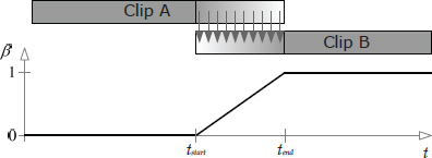
To cross-fade between two animations, we overlap the timelines of the two clips by some reasonable amount, and then blend the two clips together. The blend percentage β starts at zero at time tstart, meaning that we see only clip A when the cross-fade begins. We gradually increase β until it reaches a value of one at time tend. At this point only clip B will be visible, and we can retire clip A altogether. The time interval over which the cross-fade occurs (Δtblend = tend − tstart) is sometimes called the blend time.
Types of Cross-Fades
There are two common ways to perform a cross-blended transition:
We can also control how the blend factor β varies during the transition. In Figure 12.30 and Figure 12.31, the blend factor varied linearly with time. To achieve an even smoother transition, we could vary β according to a cubic function of time, such as a one-dimensional Bézier. When such a curve is applied to a currently running clip that is being blended out, it is known as an ease-out curve; when it is applied to a new clip that is being blended in, it is known as an ease-in curve. This is shown in Figure 12.32.

The equation for a Bézier ease-in/ease-out curve is given below. It returns the value of β at any time t within the blend interval. βstart is the blend factor at the start of the blend interval tstart, and βend is the final blend factor at time tend. The parameter u is the normalized time between tstart and tend, and for convenience we’ll also define v = 1 − u (the inverse normalized time). Note that the Bézier tangents Tstart and Tend are taken to be equal to the corresponding blend factors βstart and βend, because this yields a well-behaved curve for our purposes:
Core Poses
This is an appropriate time to mention that motion continuity can actually be achieved without blending if the animator ensures that the last pose in any given clip matches the first pose of the clip that follows it. In practice, animators often decide upon a set of core poses—for example, we might have a core pose for standing upright, one for crouching, one for lying prone and so on. By making sure that the character starts in one of these core poses at the beginning of every clip and returns to a core pose at the end, C0 continuity can be achieved by simply ensuring that the core poses match when animations are spliced together. C1 or higher-order motion continuity can also be achieved by ensuring that the character’s movement at the end of one clip smoothly transitions into the motion at the start of the next clip. This can be achieved by authoring a single smooth animation and then breaking it into two or more clips.


12.6.2.3 Directional Locomotion
LERP-based animation blending is often applied to character locomotion. When a real human being walks or runs, he can change the direction in which he is moving in two basic ways: First, he can turn his entire body to change direction, in which case he always faces in the direction he’s moving. I’ll call this pivotal movement, because the person pivots about his vertical axis when he turns. Second, he can keep facing in one direction while walking forward, backward or sideways (known as strafing in the gaming world) in order to move in a direction that is independent of his facing direction. I’ll call this targeted movement, because it is often used in order to keep one’s eye—or one’s weapon—trained on a target while moving. These two movement styles are illustrated in Figure 12.33.
Targeted Movement
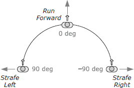
To implement targeted movement, the animator authors three separate looping animation clips—one moving forward, one strafing to the left, and one strafing to the right. I’ll call these directional locomotion clips. The three directional clips are arranged around the circumference of a semicircle, with forward at 0 degrees, left at 90 degrees and right at −90 degrees. With the character’s facing direction fixed at 0 degrees, we find the desired movement direction on the semicircle, select the two adjacent movement animations and blend them together via LERP-based blending. The blend percentage β is determined by how close the angle of movement is to the angles of two adjacent clips. This is illustrated in Figure 12.34.
Note that we did not include backward movement in our blend, for a full circular blend. This is because blending between a sideways strafe and a backward run cannot be made to look natural in general. The problem is that when strafing to the left, the character usually crosses its right foot in front of its left so that the blend into the pure forward run animation looks correct. Likewise, the right strafe is usually authored with the left foot crossing in front of the right. When we try to blend such strafe animations directly into a backward run, one leg will start to pass through the other, which looks extremely awkward and unnatural. There are a number of ways to solve this problem. One feasible approach is to define two hemispherical blends, one for forward motion and one for backward motion, each with strafe animations that have been crafted to work properly when blended with the corresponding straight run. When passing from one hemisphere to the other, we can play some kind of explicit transition animation so that the character has a chance to adjust its gait and leg crossing appropriately.
Pivotal Movement
To implement pivotal movement, we can simply play the forward locomotion loop while rotating the entire character about its vertical axis to make it turn. Pivotal movement looks more natural if the character’s body doesn’t remain bolt upright when it is turning—real humans tend to lean into their turns a little bit. We could try slightly tilting the vertical axis of the character as a whole, but that would cause problems with the inner foot sinking into the ground while the outer foot comes off the ground. A more natural-looking result can be achieved by animating three variations on the basic forward walk or run—one going perfectly straight, one making an extreme left turn and one making an extreme right turn. We can then LERP-blend between the straight clip and the extreme left turn clip to implement any desired lean angle.
12.6.3 Complex LERP Blends
In a real game engine, characters make use of a wide range of complex blends for various purposes. It can be convenient to “prepackage” certain commonly used types of complex blends for ease of use. In the following sections, we’ll investigate a few popular types of prepackaged complex blends.
12.6.3.1 Generalized One-Dimensional LERP Blending
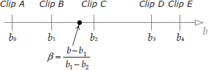
LERP blending can be easily extended to more than two animation clips, using a technique I call one-dimensional LERP blending. We define a new blend parameter b that lies in any linear range desired (e.g., from −1 to +1, or from 0 to 1, or even from 27 to 136). Any number of clips can be positioned at arbitrary points along this range, as shown in Figure 12.35. For any given value of b, we select the two clips immediately adjacent to it and blend them together using Equation (12.5). If the two adjacent clips lie at points b1 and b2, then the blend percentage β can be determined using a technique analogous to that used in Equation (12.14), as follows:

Targeted movement is just a special case of one-dimensional LERP blending. We simply straighten out the circle on which the directional animation clips were placed and use the movement direction angle θ as the parameter b (with a range of −90 to 90 degrees). Any number of animation clips can be placed onto this blend range at arbitrary angles. This is shown in Figure 12.36.
12.6.3.2 Simple Two-Dimensional LERP Blending
Sometimes we would like to smoothly vary two aspects of a character’s motion simultaneously. For example, we might want the character to be capable of aiming his weapon vertically and horizontally. Or we might want to allow our character to vary her pace length and the separation of her feet as she moves. We can extend one-dimensional LERP blending to two dimensions in order to achieve these kinds of effects.
If we know that our 2D blend involves only four animation clips, and if those clips are positioned at the four corners of a square region, then we can find a blended pose by performing two 1D blends. Our generalized blend factor b becomes a two-dimensional blend vector b = [bx by]. If b lies within the square region bounded by our four clips, we can find the resulting pose by following these steps:
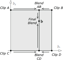
This technique is illustrated in Figure 12.37.
12.6.3.3 Triangular Two-Dimensional LERP Blending
The simple 2D blending technique we investigated in the previous section only works when the animation clips we wish to blend lie at the corners of a rectangular region. How can we blend between an arbitrary number of clips positioned at arbitrary locations in our 2D blend space?
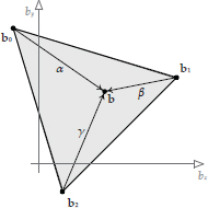
Let’s imagine that we have three animation clips that we wish to blend together. Each clip, designated by the index i, corresponds to a particular blend coordinate bi = [bix biy] in our two-dimensional blend space; these three blend coordinates form a triangle within the blend space. Each of the three clips defines a set of joint poses , where (Pi )j is the pose of joint j as defined by clip i, and N is the number of joints in the skeleton. We wish to find the interpolated pose of the skeleton corresponding to an arbitrary point b within the triangle, as illustrated in Figure 12.38.
But how can we calculate a LERP blend between three animation clips? Thankfully, the answer is simple: the LERP function can actually operate on any number of inputs, because it is really just a weighted average. As with any weighted average, the weights must add to one. In the case of a two-input LERP blend, we used the weights β and (1 − β), which of course add to one. For a three-input LERP, we simply use three weights, α, β and γ = (1 − α − β).

Then we calculate the LERP as follows:
Given the two-dimensional blend vector b, we find the blend weights α, β and γ by finding the barycentric coordinates of the point b relative to the triangle formed by the three clips in two-dimensional blend space (http://en.wikipedia.org/wiki/Barycentric_coordinates_%28mathematics%29). In general, the barycentric coordinates of a point b within a triangle with vertices b1, b2 and b3 are three scalar values (α, β, γ) that satisfy the relations
and
These are exactly the weights we seek for our three-clip weighted average. Barycentric coordinates are illustrated in Figure 12.39.
Note that plugging the barycentric coordinate (1, 0, 0) into Equation (12.17) yields b0, while (0, 1, 0) gives us b1 and (0, 0, 1) produces b2. Likewise, plugging these blend weights into Equation (12.16) gives us poses (P0)j, (P1)j and (P2)j for each joint j, respectively. Furthermore, the barycentric coordinate (, ,) lies at the centroid of the triangle and gives us an equal blend between the three poses. This is exactly what we’d expect.
12.6.3.4 Generalized Two-Dimensional LERP Blending
The barycentric coordinate technique can be extended to an arbitrary number of animation clips positioned at arbitrary locations within the two-dimensional blend space. We won’t describe it in its entirety here, but the basic idea is to use a technique known as Delaunay triangulation (http://en.wikipedia.org/wiki/Delaunay_triangulation) to find a set of triangles given the positions of the various animation clips bi. Once the triangles have been determined, we can find the triangle that encloses the desired point b and then perform a three-clip LERP blend as described above. This technique was used in FIFA soccer by EA Sports in Vancouver, implemented within their proprietary “ANT” animation framework. It is shown in Figure 12.40.
12.6.4 Partial-Skeleton Blending
A human being can control different parts of his or her body independently. For example, I can wave my right arm while walking and pointing at something with my left arm. One way to implement this kind of movement in a game is via a technique known as partial-skeleton blending.

Recall from Equations (12.5) and (12.6) that when doing regular LERP blending, the same blend percentage β was used for every joint in the skeleton. Partial-skeleton blending extends this idea by permitting the blend percentage to vary on a per-joint basis. In other words, for each joint j, we define a separate blend percentage βj. The set of all blend percentages for the entire skeleton is sometimes called a blend mask because it can be used to “mask out” certain joints by setting their blend percentages to zero.
As an example, let’s say we want our character to wave at someone using his right arm and hand. Moreover, we want him to be able to wave whether he’s walking, running or standing still. To implement this using partial blending, the animator defines three full-body animations: Walk, Run and Stand. The animator also creates a single waving animation, Wave. A blend mask is created in which the blend percentages are zero everywhere except for the right shoulder, elbow, wrist and finger joints, where they are equal to one:
When Walk, Run or Stand is LERP-blended with Wave using this blend mask, the result is a character who appears to be walking, running or standing while waving his right arm.
Partial blending is useful, but it has a tendency to make a character’s movements look unnatural. This occurs for two basic reasons:
12.6.5 Additive Blending
Additive blending approaches the problem of combining animations in a totally new way. It introduces a new kind of animation called a difference clip, which, as its name implies, represents the difference between two regular animation clips. A difference clip can be added onto a regular animation clip in order to produce interesting variations in the pose and movement of the character. In essence, a difference clip encodes the changes that need to be made to one pose in order to transform it into another pose. Difference clips are often called additive animation clips in the game industry. We’ll stick with the term difference clip in this book because it more accurately describes what is going on.
Consider two input clips called the source clip (S) and the reference clip (R). Conceptually, the difference clip is D = S − R. If a difference clip D is added to its original reference clip, we get back the source clip (S = D + R). We can also generate animations that are partway between R and S by adding a percentage of D to R, in much the same way that LERP blending finds intermediate animations between two extremes. However, the real beauty of the additive blending technique is that once a difference clip has been created, it can be added to other unrelated clips, not just to the original reference clip. We’ll call these animations target clips and denote them with the symbol T.
As an example, if the reference clip has the character running normally and the source clip has him running in a tired manner, then the difference clip will contain only the changes necessary to make the character look “tired” while running. If this difference clip is now applied to a clip of the character walking, the resulting animation can make the character look tired while walking. A whole host of interesting and very natural-looking animations can be created by adding a single difference clip onto various “regular” animation clips, or a collection of difference clips can be created, each of which produces a different effect when added to a single target animation.
12.6.5.1 Mathematical Formulation
A difference animation D is defined as the difference between some source animation S and some reference animation R. So conceptually, the difference pose (at a single point in time) is D = S − R. Of course, we’re dealing with joint poses, not scalar quantities, so we cannot simply subtract the poses. In general, a joint pose is a 4 × 4 affine transformation matrix that transforms points and vectors from the child joint’s local space to the space of its parent joint. The matrix equivalent of subtraction is multiplication by the inverse matrix. So given the source pose Sj and the reference pose Rj for any joint j in the skeleton, we can define the difference pose Dj at that joint as follows. (For this discussion, we’ll drop the C − P or j − p(j) subscript, as it is understood that we are dealing with child-to-parent pose matrices.)
“Adding” a difference pose Dj onto a target pose Tj yields a new additive pose Aj. This is achieved by simply concatenating the difference transform and the target transform as follows:
We can verify that this is correct by looking at what happens when the difference pose is “added” back onto the original reference pose:
In other words, adding the difference animation D back onto the original reference animation R yields the source animation S, as we’d expect.
Temporal Interpolation of Difference Clips
As we learned in Section 12.4.1.1, game animations are almost never sampled on integer frame indices. To find a pose at an arbitrary time t, we must often temporally interpolate between adjacent pose samples at times t1 and t2. Thankfully, difference clips can be temporally interpolated just like their non-additive counterparts. We can simply apply Equations (12.12) and (12.14) directly to our difference clips as if they were ordinary animations.
Note that a difference animation can only be found when the input clips S and R are of the same duration. Otherwise there would be a period of time during which either S or R is undefined, meaning D would be undefined as well.
Additive Blend Percentage
In games, we often wish to blend in only a percentage of a difference animation to achieve varying degrees of the effect it produces. For example, if a difference clip causes the character to turn his head 80 degrees to the right, blending in 50% of the difference clip should make him turn his head only 40 degrees to the right.
To accomplish this, we turn once again to our old friend LERP. We wish to interpolate between the unaltered target animation and the new animation that would result from a full application of the difference animation. To do this, we extend Equation (12.18) as follows:
As we saw in Chapter 5, we cannot LERP matrices directly. So Equation (11.16) must be broken down into three separate interpolations for S, Q and T, just as we did in Equations (12.7) through (12.11).
12.6.5.2 Additive Blending versus Partial Blending
Additive blending is similar in some ways to partial blending. For example, we can take the difference between a standing clip and a clip of standing while waving the right arm. The result will be almost the same as using a partial blend to make the right arm wave. However, additive blends suffer less from the “disconnected” look of animations combined via partial blending. This is because, with an additive blend, we are not replacing the animation for a subset of joints or interpolating between two potentially unrelated poses. Rather, we are adding movement to the original animation—possibly across the entire skeleton. In effect, a difference animation “knows” how to change a character’s pose in order to get him to do something specific, like being tired, aiming his head in a certain direction, or waving his arm. These changes can be applied to a reasonably wide variety of animations, and the result often looks very natural.
12.6.5.3 Limitations of Additive Blending
Of course, additive animation is not a silver bullet. Because it adds movement to an existing animation, it can have a tendency to over-rotate the joints in the skeleton, especially when multiple difference clips are applied simultaneously. As a simple example, imagine a target animation in which the character’s left arm is bent at a 90 degree angle. If we add a difference animation that also rotates the elbow by 90 degrees, then the net effect would be to rotate the arm by 90 + 90 = 180 degrees. This would cause the lower arm to interpenetrate the upper arm—not a comfortable position for most individuals!
Clearly we must be careful when selecting the reference clip and also when choosing the target clips to which to apply it. Here are some simple rules of thumb:
These rules of thumb can be a helpful starting point, but the only way to really learn how to create and apply difference clips is by trial and error or by apprenticing with animators or engineers who have experience creating and applying difference animations. If your team hasn’t used additive blending in the past, expect to spend a significant amount of time learning the art of additive blending.
12.6.6 Applications of Additive Blending
12.6.6.1 Stance Variation
One particularly striking application of additive blending is stance variation. For each desired stance, the animator creates a one-frame difference animation. When one of these single-frame clips is additively blended with a base animation, it causes the entire stance of the character to change drastically while he continues to perform the fundamental action he’s supposed to perform. This idea is illustrated in Figure 12.41.

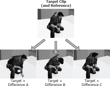
12.6.6.2 Locomotion Noise
Real humans don’t run exactly the same way with every footfall—there is variation in their movement over time. This is especially true if the person is distracted (for example, by attacking enemies). Additive blending can be used to layer randomness, or reactions to distractions, on top of an otherwise entirely repetitive locomotion cycle. This is illustrated in Figure 12.42.
12.6.6.3 Aim and Look-At
Another common use for additive blending is to permit the character to look around or to aim his weapon. To accomplish this, the character is first animated doing some action, such as running, with his head or weapon facing straight ahead. Then the animator changes the direction of the head or the aim of the weapon to the extreme right and saves off a one-frame or multiframe difference animation. This process is repeated for the extreme left, up and down directions. These four difference animations can then be additively blended onto the original straight-ahead animation clip, causing the character to aim right, left, up, down or anywhere in between.
The angle of the aim is governed by the additive blend factor of each clip. For example, blending in 100% of the right additive causes the character to aim as far right as possible. Blending 50% of the left additive causes him to aim at an angle that is one-half of his leftmost aim. We can also combine this with an up or down additive to aim diagonally. This is demonstrated in Figure 12.43.

12.6.6.4 Overloading the Time Axis
It’s interesting to note that the time axis of an animation clip needn’t be used to represent time. For example, a three-frame animation clip could be used to provide three aim poses to the engine—a left aim pose on frame 1, a forward aim pose on frame 2 and a right aim pose on frame 3. To make the character aim to the right, we can simply fix the local clock of the aim animation on frame 3. To perform a 50% blend between aiming forward and aiming right, we can dial in frame 2.5. This is a great example of leveraging existing features of the engine for new purposes.
12.7 Post-Processing
Once a skeleton has been posed by one or more animation clips and the results have been blended together using linear interpolation or additive blending, it is often necessary to modify the pose prior to rendering the character. This is called animation post-processing. In this section, we’ll look at a few of the most common kinds of animation post-processing.
12.7.1 Procedural Animations
A procedural animation is any animation generated at runtime rather than being driven by data exported from an animation tool such as Maya. Sometimes, hand-animated clips are used to pose the skeleton initially, and then the pose is modified in some way via procedural animation as a post-processing step. A procedural animation can also be used as an input to the system in place of a hand-animated clip.
For example, imagine that a regular animation clip is used to make a vehicle appear to be bouncing up and down on the terrain as it moves. The direction in which the vehicle travels is under player control. We would like to adjust the rotation of the front wheels and steering wheel so that they move convincingly when the vehicle is turning. This can be done by post-processing the pose generated by the animation. Let’s assume that the original animation has the front tires pointing straight ahead and the steering wheel in a neutral position. We can use the current angle of turn to create a quaternion about the vertical axis that will deflect the front tires by the desired amount. This quaternion can be multiplied with the front tire joints’ Q channel to produce the final pose of the tires. Likewise, we can generate a quaternion about the axis of the steering column and multiply it into the steering wheel joint’s Q channel to deflect it. These adjustments are made to the local pose, prior to global pose calculation and matrix palette generation (see Section 12.5).
As another example, let’s say that we wish to make the trees and bushes in our game world sway naturally in the wind and get brushed aside when characters move through them. We can do this by modeling the trees and bushes as skinned meshes with simple skeletons. Procedural animation can be used, in place of or in addition to hand-animated clips, to cause the joints to move in a natural-looking way. We might apply one or more sinusoids, or a Perlin noise function, to the rotation of various joints to make them sway in the breeze, and when a character moves through a region containing a bush or grass, we can deflect its root joint quaternion radially outward to make it appear to be pushed over by the character.
12.7.2 Inverse Kinematics
Let’s say we have an animation clip in which a character leans over to pick up an object from the ground. In Maya, the clip looks great, but in our production game level, the ground is not perfectly flat, so sometimes the character’s hand misses the object or appears to pass through it. In this case, we would like to adjust the final pose of the skeleton so that the hand lines up exactly with the target object. A technique known as inverse kinematics (IK) can be used to make this happen.

A regular animation clip is an example of forward kinematics (FK). In forward kinematics, the input is a set of local joint poses, and the output is a global pose and a skinning matrix for each joint. Inverse kinematics goes in the other direction: The input is the desired global pose of a single joint, which is known as the end effector. We solve for the local poses of other joints in the skeleton that will bring the end effector to the desired location.
Mathematically, IK boils down to an error minimization problem. As with most minimization problems, there might be one solution, many or none at all. This makes intuitive sense: If I try to reach a doorknob that is on the other side of the room, I won’t be able to reach it without walking over to it. IK works best when the skeleton starts out in a pose that is reasonably close to the desired target. This helps the algorithm to focus in on the “closest” solution and to do so in a reasonable amount of processing time. Figure 12.44 shows IK in action.
Imagine a two-joint skeleton, each of which can rotate only about a single axis. The rotation of these two joints can be described by a two-dimensional angle vector θ = [θ1 θ2]. The set of all possible angles for our two joints forms a two-dimensional space called configuration space. Obviously, for more complex skeletons with more degrees of freedom per joint, configuration space becomes multidimensional, but the concepts described here work equally well no matter how many dimensions we have.
Now imagine plotting a three-dimensional graph, where for each combination of joint rotations (i.e., for each point in our two-dimensional configuration space), we plot the distance from the end effector to the desired target. An example of this kind of plot is shown in Figure 12.45. The “valleys” in this three-dimensional surface represent regions in which the end effector is as close as possible to the target. When the height of the surface is zero, the end effector has reached its target. Inverse kinematics, then, attempts to find minima (low points) on this surface.

We won’t get into the details of solving the IK minimization problem here. You can read more about IK at http://en.wikipedia.org/wiki/Inverse_kinematics and in Jason Weber’s article, “Constrained Inverse Kinematics” [47].
12.7.3 Rag Dolls
A character’s body goes limp when he dies or becomes unconscious. In such situations, we want the body to react in a physically realistic way with its surroundings. To do this, we can use a rag doll. A rag doll is a collection of physically simulated rigid bodies, each one representing a semi-rigid part of the character’s body, such as his lower arm or his upper leg. The rigid bodies are constrained to one another at the joints of the character in such a way as to produce natural-looking “lifeless” body movement. The positions and orientations of the rigid bodies are determined by the physics system and are then used to drive the positions and orientations of certain key joints in the character’s skeleton. The transfer of data from the physics system to the skeleton is typically done as a post-processing step.
To really understand rag doll physics, we must first have an understanding of how the collision and physics systems work. Rag dolls are covered in more detail in Sections 13.4.8.7 and 13.5.3.8.
12.8 Compression Techniques
Animation data can take up a lot of memory. A single joint pose might be composed of ten floating-point channels (three for translation, four for rotation and up to three more for scale). Assuming each channel contains a 4-byte floating-point value, a one-second clip sampled at 30 samples per second would occupy 4 bytes × 10 channels × 30 samples/second = 1200 bytes per joint per second, or a data rate of about 1.17 KiB per joint per second. For a 100-joint skeleton (which is small by today’s standards), an uncompressed animation clip would occupy 117 KiB per joint per second. If our game contained 1,000 seconds of animation (which is on the low side for a modern game), the entire dataset would occupy a whopping 114.4 MiB. That’s quite a lot, considering that a PlayStation 3 has only 256 MiB of main RAM and 256 MiB of video RAM. Sure, the PS4 has 8 GiB of RAM. But even so—we would rather have much richer animations with a lot more variety than waste memory unnecessarily. Therefore, game engineers invest a significant amount of effort into compressing animation data in order to permit the maximum richness and variety of movement at the minimum memory cost.
12.8.1 Channel Omission
One simple way to reduce the size of an animation clip is to omit channels that are irrelevant. Many characters do not require nonuniform scaling, so the three scale channels can be reduced to a single uniform scale channel. In some games, the scale channel can actually be omitted altogether for all joints (except possibly the joints in the face). The bones of a humanoid character generally cannot stretch, so translation can often be omitted for all joints except the root, the facial joints and sometimes the collar bones. Finally, because quaternions are always normalized, we can store only three components per quat (e.g., x, y and z) and reconstruct the fourth component (e.g., w) at runtime.
As a further optimization, channels whose pose does not change over the course of the entire animation can be stored as a single sample at time t = 0 plus a single bit indicating that the channel is constant for all other values of t.
Channel omission can significantly reduce the size of an animation clip. A 100-joint character with no scale and no translation requires only 303 channels—three channels for the quaternions at each joint, plus three channels for the root joint’s translation. Compare this to the 1,000 channels that would be required if all ten channels were included for all 100 joints.
12.8.2 Quantization
Another way to reduce the size of an animation is to reduce the size of each channel. A floating-point value is normally stored in 32-bit IEEE format. This format provides 23 bits of precision in the mantissa and an 8-bit exponent. However, it’s often not necessary to retain that kind of precision and range in an animation clip. When storing a quaternion, the channel values are guaranteed to lie in the range [−1, 1]. At a magnitude of 1, the exponent of a 32-bit IEEE float is zero, and 23 bits of precision give us accuracy down to the seventh decimal place. Experience shows that a quaternion can be encoded well with only 16 bits of precision, so we’re really wasting 16 bits per channel if we store our quats using 32-bit floats.
Converting a 32-bit IEEE float into an n-bit integer representation is called quantization. There are actually two components to this operation: Encoding is the process of converting the original floating-point value to a quantized integer representation. Decoding is the process of recovering an approximation to the original floating-point value from the quantized integer. (We can only recover an approximation to the original data—quantization is a lossy compression method because it effectively reduces the number of bits of precision used to represent the value.)
To encode a floating-point value as an integer, we first divide the valid range of possible input values into N equally sized intervals. We then determine within which interval a particular floating-point value lies and represent that value by the integer index of its interval. To decode this quantized value, we simply convert the integer index into floating-point format and shift and scale it back into the original range. N is usually chosen to correspond to the range of possible integer values that can be represented by an n-bit integer. For example, if we’re encoding a 32-bit floating-point value as a 16-bit integer, the number of intervals would be N = 216 = 65,536.
Jonathan Blow wrote an excellent article on the topic of floating-point scalar quantization in the Inner Product column of Game Developer Magazine, available at https://bit.ly/2J92oiU. The article presents two ways to map a floating-point value to an interval during the encoding process: We can either truncate the float to the next lowest interval boundary (T encoding), or we can round the float to the center of the enclosing interval (R encoding). Likewise, it describes two approaches to reconstructing the floating-point value from its integer representation: We can either return the value of the left-hand side of the interval to which our original value was mapped (L reconstruction), or we can return the value of the center of the interval (C reconstruction). This gives us four possible encode/decode methods: TL, TC, RL and RC. Of these, TL and RC are to be avoided because they tend to remove or add energy to the dataset, which can often have disastrous effects. TC has the benefit of being the most efficient method in terms of bandwidth, but it suffers from a severe problem—there is no way to represent the value zero exactly. (If you encode 0.0f, it becomes a small positive value when decoded.) RL is therefore usually the best choice and is the method we’ll demonstrate here.
The article only talks about quantizing positive floating-point values, and in the examples, the input range is assumed to be [0, 1] for simplicity. However, we can always shift and scale any floating-point range into the range [0, 1]. For example, the range of quaternion channels is [−1, 1], but we can convert this to the range [0, 1] by adding one and then dividing by two.
The following pair of routines encode and decode an input floating-point value lying in the range [0, 1] into an n-bit integer, according to Jonathan Blow’s RL method. The quantized value is always returned as a 32-bit unsigned integer (U32), but only the least-significant n bits are actually used, as specified by the nBits argument. For example, if you pass nBits==16, you can safely cast the result to a U16.
U32 CompressUnitFloatRL(F32 unitFloat, U32 nBits)
{
 // Determine the number of intervals based on the
 // number of output bits we’ve been asked to produce.
 U32 nIntervals = 1u ≪ nBits;
 // Scale the input value from the range [0, 1] into
 // the range [0, nIntervals − 1]. We subtract one
 // interval because we want the largest output value
 // to fit into nBits bits.
 F32 scaled = unitFloat * (F32)(nIntervals − 1u);
 // Finally, round to the nearest interval center. We
 // do this by adding 0.5f and then truncating to the
 // next-lowest interval index (by casting to U32).
 U32 rounded = (U32)(scaled + 0.5f);
 // Guard against invalid input values.
 if (rounded > nIntervals − 1u)
 rounded = nIntervals − 1u;
 return rounded;
}
F32 DecompressUnitFloatRL(U32 quantized, U32 nBits)
{
 // Determine the number of intervals based on the
 // number of bits we used when we encoded the value.
 U32 nIntervals = 1u ≪ nBits;
 // Decode by simply converting the U32 to an F32, and
 // scaling by the interval size.
 F32 intervalSize = 1.0f / (F32)(nIntervals − 1u);
 F32 approxUnitFloat = (F32)quantized * intervalSize;
 return approxUnitFloat;
}
To handle arbitrary input values in the range [min, max], we can use these routines:
U32 CompressFloatRL(F32 value, F32 min, F32 max,
   U32 nBits)
{
 F32 unitFloat = (value - min) / (max - min);
 U32 quantized = CompressUnitFloatRL(unitFloat,
    nBits);
 return quantized;
}
F32 DecompressFloatRL(U32 quantized, F32 min, F32 max,
   U32 nBits)
{
 F32 unitFloat = DecompressUnitFloatRL(quantized,
    nBits);
 F32 value = min + (unitFloat * (max - min));
 return value;
}
Let’s return to our original problem of animation channel compression. To compress and decompress a quaternion’s four components into 16 bits per channel, we simply call CompressFloatRL() and DecompressFloatRL() with min = −1, max = 1 and n = 16:
inline U16 CompressRotationChannel(F32 qx)
{
 return (U16)CompressFloatRL(qx, −1.0f, 1.0f, 16u);
}
inline F32 DecompressRotationChannel(U16 qx)
{
 return DecompressFloatRL((U32)qx, −1.0f, 1.0f, 16u);
}
Compression of translation channels is a bit trickier than rotations, because unlike quaternion channels, the range of a translation channel could theoretically be unbounded. Thankfully, the joints of a character don’t move very far in practice, so we can decide upon a reasonable range of motion and flag an error if we ever see an animation that contains translations outside the valid range. In-game cinematics are an exception to this rule—when an IGC is animated in world space, the translations of the characters’ root joints can grow very large. To address this, we can select the range of valid translations on a per-animation or per-joint basis, depending on the maximum translations actually achieved within each clip. Because the data range might differ from animation to animation, or from joint to joint, we must store the range with the compressed clip data. This will add a tiny amount of data to each animation clip, but the impact is generally negligible.
// We’ll use a 2 m range -- your mileage may vary.
F3 2 MAX_TRANSLATION = 2.0f;
inline U16 CompressTranslationChannel(F32 vx)
{
 // Clamp to valid range…
 if (vx < −MAX_TRANSLATION)
  vx = −MAX_TRANSLATION;
 if (vx > MAX_TRANSLATION)
  vx = MAX_TRANSLATION;
 return (U16)CompressFloatRL(vx,
   −MAX_TRANSLATION, MAX_TRANSLATION, 16);
}
inline F32 DecompressTranslationChannel(U16 vx)
{
 return DecompressFloatRL((U32)vx,
   −MAX_TRANSLATION, MAX_TRANSLATION, 16);
}
12.8.3 Sampling Frequency and Key Omission
Animation data tends to be large for three reasons: first, because the pose of each joint can contain upwards of ten channels of floating-point data; second, because a skeleton contains a large number of joints (250 or more for a humanoid character on PS3 or Xbox 360, and more than 800 on some PS4 and Xbox One games); third, because the pose of the character is typically sampled at a high rate (e.g., 30 frames per second). We’ve seen some ways to address the first problem. We can’t really reduce the number of joints for our high-resolution characters, so we’re stuck with the second problem. To attack the third problem, we can do two things:
The latter technique is a bit involved, and it requires us to store information about the time of each sample. This additional data can erode the savings we achieved by omitting samples in the first place. However, some game engines have used this technique successfully.
12.8.4 Curve-Based Compression
One of the most powerful, easiest-to-use and best-thought-out animation APIs I’ve ever worked with is Granny, by Rad Game Tools. Granny stores animations not as a regularly spaced sequence of pose samples but as a collection of nth-order, nonuniform, nonrational B-splines, describing the paths of a joint’s S, Q and T channels over time. Using B-splines allows channels with a lot of curvature to be encoded using only a few data points.
Granny exports an animation by sampling the joint poses at regular intervals, much like traditional animation data. For each channel, Granny then fits a set of B-splines to the sampled dataset to within a user-specified tolerance. The end result is an animation clip that is usually significantly smaller than its uniformly sampled, linearly interpolated counterpart. This process is illustrated in Figure 12.46.

12.8.5 Wavelet Compression
Another way to compress animation data is to apply signal processing theory to the problem, via a technique known as wavelet compression. A wavelet is a function whose amplitude oscillates like a wave but whose duration is very short, like a brief ripple in a pond. Wavelet functions are carefully crafted to give them desirable properties for use in signal processing.
In wavelet compression, an animation curve is decomposed into a sum of orthonormal wavelets, in much the same way that an arbitrary signal can be represented as a train of delta functions or a sum of sinusoids. We discuss signal processing and linear time-invariant systems in some depth in Section 14.2; the concepts presented there form the foundations necessary to understand wavelet compression. A full discussion of wavelet-based compression techniques is well beyond the scope of this book, but you can read more about it online. Search for “wavelet” to find introductory articles on the topic, and then try searching for “Animation Compression: Signal Processing” on Nicholas Frechette’s blog for a great article on how wavelet compression was implemented for Thief (2014) by Eidos Montreal.
12.8.6 Selective Loading and Streaming
The cheapest animation clip is the one that isn’t in memory at all. Most games don’t need every animation clip to be in memory simultaneously. Some clips apply only to certain classes of character, so they needn’t be loaded during levels in which that class of character is never encountered. Other clips apply to one-off moments in the game. These can be loaded or streamed into memory just before being needed and dumped from memory once they have played.
Most games load a core set of animation clips into memory when the game first boots and keep them there for the duration of the game. These include the player character’s core move set and animations that apply to objects that reappear over and over throughout the game, such as weapons or power-ups. All other animations are usually loaded on an as-needed basis. Some game engines load animation clips individually, but many package them together into logical groups that can be loaded and unloaded as a unit.
12.9 The Animation Pipeline
The operations performed by the low-level animation engine form a pipeline that transforms its inputs (animation clips and blend specifications) into the desired outputs (local and global poses, plus a matrix palette for rendering).
For each animating character and object in the game, the animation pipeline takes one or more animation clips and corresponding blend factors as input, blends them together, and generates a single local skeletal pose as output. It also calculates a global pose for the skeleton and a palette of skinning matrices for use by the rendering engine. Post-processing hooks are usually provided, which permit the local pose to be modified prior to final global pose and matrix palette generation. This is where inverse kinematics (IK), rag doll physics and other forms of procedural animation are applied to the skeleton. The stages of this pipeline are:
A typical animation pipeline is depicted in Figure 12.47.
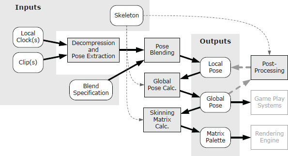
12.10 Action State Machines
The actions of a game character (standing, walking, running, jumping, etc.) are usually best modeled via a finite state machine, commonly known as the action state machine (ASM). The ASM subsystem sits atop the animation pipeline and provides a state-driven animation interface for use by virtually all higher-level game code.
Each state in an ASM corresponds to an arbitrarily complex blend of simultaneous animation clips. Some states might be very simple—for example, the “idle” state might be comprised of a single full-body animation. Other states might be more complex. A “running” state might correspond to a semicircular blend, with strafing left, running forward and strafing right at the −90 degree, 0 degree and +90 degree points, respectively. The “running while shooting” state might include a semicircular directional blend, plus additive or partial-skeleton blend nodes for aiming the character’s weapon up, down, left and right, and additional blends to permit the character to look around with its eyes, head and shoulders. More additive animations might be included to control the character’s overall stance, gait and foot spacing while locomoting and to provide a degree of “humanness” through random movement variations.
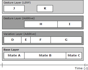
A character’s ASM also ensures that characters can transition smoothly from state to state. During a transition from state A to state B, the final output poses of both states are usually blended together to provide a smooth cross-fade between them.
Most high-quality animation engines also permit different parts of a character’s body to be doing different, independent or semi-independent actions simultaneously. For instance, a character might be running, aiming and firing a weapon with its arms, and speaking a line of dialog with its facial joints. The movements of different parts of the body aren’t generally in perfect sync either—certain parts of the body tend to “lead” the movements of other parts (e.g., the head leads a turn, followed by the shoulders, the hips and finally the legs). In traditional animation, this well-known technique is known as anticipation [51]. This kind of complex movement can be realized by allowing multiple independent state machines to control a single character. Usually each state machine exists in a separate state layer, as shown in Figure 12.48. The output poses from each layer’s ASM are blended together into a final composite pose.
All of this means that at any given moment in time, multiple animation clips are contributing to the final pose of a character’s skeleton. For each character, then, we need a way to track all of the currently-playing clips, and to describe how exactly they should be blended together in order to produce the character’s final pose. Generally speaking, there are two ways to do this:
12.10.1 The Flat Weighted Average Approach
In the flat weighted average approach, every animation clip that is currently playing on a given character is associated with a blend weight indicating how much it should contribute to its final pose. A flat list of all active animation clips (i.e., clips whose blend weights are nonzero) is maintained. To calculate the final pose of the skeleton, we extract a pose at the appropriate time index for each of the N active clips. Then, for each joint of the skeleton, we calculate a simple N-point weighted average of the translation vectors, rotation quaternions and scale factors extracted from the N active animations. This yields the final pose of the skeleton.
The equation for the weighted average of a set of N vectors {vi} is as follows:
If the weights are normalized, meaning they sum to one, then this equation can be simplified to the following:
In the case of N = 2, if we let w0 = (1 − β) and w1 = β, the weighted average reduces to the familiar equation for the linear interpolation (LERP) between two vectors:
We can apply this same weighted average formulation equally well to quaternions by simply treating them as four-element vectors.
12.10.1.1 Example: OGRE
The OGRE animation system works in exactly this way. An Ogre::Entity represents an instance of a 3D mesh (e.g., one particular character walking around in the game world). The Entity aggregates an object called an Ogre∷AnimationStateSet, which in turn maintains a list of Ogre∷AnimationState objects, one for each active animation. The Ogre∷AnimationState class is shown in the code snippet below. (A few irrelevant details have been omitted for clarity.)
/** Represents the state of an animation clip and the
 weight of its influence on the overall pose of the
 character.
*/
class AnimationState
{
protected:
 String  mAnimationName; // reference to
 // clip
 Real  mTimePos; // local clock
 Real  mWeight; // blend weight
 bool  mEnabled; // is this anim
   // running?
 bool  mLoop; // should the
   // anim loop?
public:
 /// API functions…
};
Each AnimationState keeps track of one animation clip’s local clock and its blend weight. When calculating the final pose of the skeleton for a particular Ogre::Entity, OGRE’s animation system simply loops through each active AnimationState in its AnimationStateSet. A skeletal pose is extracted from the animation clip corresponding to each state at the time index specified by that state’s local clock. For each joint in the skeleton, an N-point weighted average is then calculated for the translation vectors, rotation quaternions and scales, yielding the final skeletal pose.
It is interesting to note that OGRE has no concept of a playback rate (R). If it did, we would have expected to see a data member like this in the Ogre∷AnimationState class:
Real mPlaybackRate;
Of course, we can still make animations play more slowly or more quickly in OGRE by simply scaling the amount of time we pass to the addTime() function, but unfortunately, OGRE does not support animation time scaling out of the box.
12.10.1.2 Example: Granny
The Granny animation system, by Rad Game Tools (http://www.radgametool.com/granny.html), provides a flat, weighted average animation blending system similar to OGRE’s. Granny permits any number of animations to be played on a single character simultaneously. The state of each active animation is maintained in a data structure known as a granny_control. Granny calculates a weighted average to determine the final pose, automatically normalizing the weights of all active clips. In this sense, its architecture is virtually identical to that of OGRE’s animation system.
Where Granny really shines is in its handling of time. Granny uses the global clock approach discussed in Section 12.4.3. It allows each clip to be looped an arbitrary number of times or infinitely. Clips can also be time-scaled; a negative time scale allows an animation to be played in reverse.
12.10.1.3 Cross-Fades with a Flat Weighted Average
In an animation engine that employs the flat weighted average architecture, cross-fades are implemented by adjusting the weights of the clips themselves. Recall that any clip whose weight wi = 0 will not contribute to the current pose of the character, while those whose weights are nonzero are averaged together to generate the final pose. If we wish to transition smoothly from clip A to clip B, we simply ramp up clip B’s weight wB, while simultaneously ramping down clip A’s weight wA. This is illustrated in Figure 12.49.
Cross-fading in a weighted average architecture becomes a bit trickier when we wish to transition from one complex blend to another. As an example, let’s say we wish to transition the character from walking to jumping. Let’s assume that the walk movement is produced by a three-way average between clips A, B and C, and that the jump movement is produced by a two-way average between clips D and E.
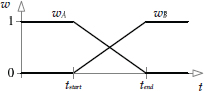
We want the character to look like he’s smoothly transitioning from walking to jumping, without affecting how the walk or jump animations look individually. So during the transition, we want to ramp down the ABC clips and ramp up the DE clips while keeping the relative weights of the ABC and DE clip groups constant. If the cross-fade’s blend factor is denoted by λ, we can meet this requirement by simply setting the weights of both clip groups to their desired values and then multiplying the weights of the source group by (1 − λ) and the weights of the destination group by λ.
Let’s look at a concrete example to convince ourselves that this will work properly. Imagine that before the transition from ABC to DE, the nonzero weights are as follows: wA = 0.2, wB = 0.3 and wC = 0.5. After the transition, we want the nonzero weights to be wD = 0.33 and wE = 0.66. So, we set the weights as follows:
From Equations (12.20), you should be able to convince yourself of the following:
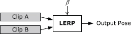
For this approach to work, the implementation must keep track of the logical groupings between clips (even though, at the lowest level, all of the clips’ states are maintained in one big, flat array—for example, the Ogre∷AnimationStateSet in OGRE). In our example above, the system must “know” that A, B and C form a group, that D and E form another group, and that we wish to transition from group ABC to group DE. This requires additional metadata to be maintained, on top of the flat array of clip states.
12.10.2 Blend Trees
Some animation engines represent a character’s clip state not as a flat weighted average but rather as a tree of blend operations. An animation blend tree is an example of what is known in compiler theory as an expression tree or a syntax tree. The interior nodes of such a tree are operators, and the leaf nodes serve as the inputs to those operators. (More correctly, the interior nodes represent the nonterminals of the grammar, while the leaf nodes represent the terminals.)
In the following sections, we’ll briefly revisit the various kinds of animation blends we learned about in Sections 12.6.3 and 12.6.5 and see how each can be represented by an expression tree.
12.10.2.1 Binary LERP Blend Trees
As we saw in Section 12.6.1, a binary linear interpolation (LERP) blend takes two input poses and blends them together into a single output pose. A blend weight β controls the percentage of the second input pose that should appear at the output, while (1 − β) specifies the percentage of the first input pose. This can be represented by the binary expression tree shown in Figure 12.50.
12.10.2.2 Generalized One-Dimensional Blend Trees
In Section 12.6.3.1, we learned that it can be convenient to define a generalized one-dimensional LERP blend by placing an arbitrary number of clips along a linear scale. A blend factor b specifies the desired blend along this scale. Such a blend can be pictured as an n-input operator, as shown in Figure 12.51.
Given a specific value for b, such a linear blend can always be transformed into a binary LERP blend. We simply use the two clips immediately adjacent to b as the inputs to the binary blend and calculate the blend weight β as specified in Equation (12.15)
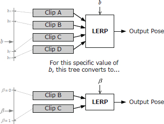

12.10.2.3 Two-Dimensional LERP Blend Trees
In Section 12.6.3.2, we saw how a two-dimensional LERP blend can be realized by simply cascading the results of two binary LERP blends. Given a desired two-dimensional blend point b = [bx by], Figure 12.52 shows how this kind of blend can be represented in tree form.
12.10.2.4 Additive Blend Trees
Section 12.6.5 described additive blending. This is a binary operation, so it can be represented by a binary tree node, as shown in Figure 12.53. A single blend weight β controls the amount of the additive animation that should appear at the output—when β = 0, the additive clip does not affect the output at all, while when β = 1, the additive clip has its maximum effect on the output.

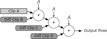
Additive blend nodes must be handled carefully, because the inputs are not interchangeable (as they are with most types of blend operators). One of the two inputs is a regular skeletal pose, while the other is a special kind of pose known as a difference pose (also known as an additive pose). A difference pose may only be applied to a regular pose, and the result of an additive blend is another regular pose. This implies that the additive input of a blend node must always be a leaf node, while the regular input may be a leaf or an interior node. If we want to apply more than one additive animation to our character, we must use a cascaded binary tree with the additive clips always applied to the additive inputs, as shown in Figure 12.54.
12.10.2.5 Layered Blend Trees
We said at the beginning of Section 12.10 that complex character movement can be produced by arranging multiple independent state machines into state layers. The output poses from each layer’s ASM are blended together into a final composite pose. When this is implemented using blend trees, the net effect is to combine the blend trees of each active state together into one über tree, as illustrated in Figure 12.55.

12.10.2.6 Cross-Fades with Blend Trees
As a character transitions from state to state within each layer of a layered ASM, we often wish to provide a smooth cross-fade between states. Implementing a cross-fade in an expression tree based ASM is a bit more intuitive than it is in a weighted average architecture. Whether we’re transitioning from one clip to another or from one complex blend to another, the approach is always the same: We simply introduce a transient binary LERP node between the roots of the blend trees of each state to handle the cross-fade.
We’ll denote the blend factor of the cross-fade node with the symbol λ as before. Its top input is the source state’s blend tree (which can be a single clip or a complex blend), and its bottom input is the destination state’s tree (again a clip or a complex blend). During the transition, λ is ramped from zero to one. Once λ = 1, the transition is complete, and the cross-fade LERP node and its top input tree can be retired. This leaves its bottom input tree as the root of the overall blend tree for the given state layer, thus completing the transition. This process is illustrated in Figure 12.56.

12.10.3 State and Blend Tree Specifications
Animators, game designers and programmers usually cooperate to create the animation and control systems for the central characters in a game. These developers need a way to specify the states that make up a character’s ASM, to lay out the tree structure of each blend tree, and to select the clips that will serve as their inputs. Although the states and blend trees could be hard-coded, most modern game engines provide a data-driven means of defining animation states. The goal of a data-driven approach is to permit a user to create new animation states, remove unwanted states, fine-tune existing states and then see the effects of his or her changes reasonably quickly. In other words, the central goal of a data-driven animation engine is to enable rapid iteration.
To build an arbitrarily complex blend tree, we really only require four atomic types of blend nodes: clips, binary LERP blends, binary additive blends and possibly ternary (triangular) LERP blends. Virtually any blend tree imaginable can be created as compositions of these atomic nodes.
A blend tree built exclusively from atomic nodes can quickly become large and unwieldy. As a result, many game engines permit custom compound node types to be predefined for convenience. The N-dimensional linear blend node discussed in Sections 12.6.3.4 and 12.10.2.2 is an example of a compound node. One can imagine myriad complex blend node types, each one addressing a particular problem specific to the particular game being made. A soccer game might define a node that allows the character to dribble the ball. A war game could define a special node that handles aiming and firing a weapon. A brawler could define custom nodes for each fight move the characters can perform. Once we have the ability to define custom node types, the sky’s the limit.
The means by which the users enter animation state data varies widely. Some game engines employ a simple, bare-bones approach, allowing animation states to be specified in a text file with a simple syntax. Other engines provide a slick, graphical editor that permits animation states to be constructed by dragging atomic components such as clips and blend nodes onto a canvas and linking them together in arbitrary ways. Such editors usually provide a live preview of the character so that the user can see immediately how the character will look in the final game. In my opinion, the specific method chosen has little bearing on the quality of the final game—what matters most is that the user can make changes and see the results of those changes reasonably quickly and easily.
12.10.3.1 Example: The Naughty Dog Engine
The animation engine used in Naughty Dog’s Uncharted and The Last of Us franchises employs a simple, text-based approach to specifying animation states. For reasons related to Naughty Dog’s rich history with the Lisp language (see Section 16.9.5.1), state specifications in the Naughty Dog engine are written in a customized version of the Scheme programming language (which itself is a Lisp variant). Two basic state types can be used: simple and complex.
Simple States
A simple state contains a single animation clip. For example:
(define-state simple
 :name “pirate-b-bump-back”
 :clip “pirate-b-bump-back”
 :flags (anim-state-flag no-adjust-to-ground)
)
Don’t let the Lisp-style syntax throw you. All this block of code does is to define a state named “pirate-b-bump-back” whose animation clip also happens to be named “pirate-b-bump-back.” The :flags parameter allows users to specify various Boolean options on the state.
Complex States
A complex state contains an arbitrary tree of LERP or additive blends. For example, the following state defines a tree that contains a single binary LERP blend node, with two clips (“walk-l-to-r” and “run-l-to-r”) as its inputs:
(define-state complex
 :name “move-l-to-r”
 :tree
  (anim-node-lerp
   (anim-node-clip “walk-1-to-r”)
   (anim-node-clip “run-1-to-r”)
  )
)
The :tree argument allows the user to specify an arbitrary blend tree, composed of LERP or additive blend nodes and nodes that playindividual animation clips.
From this, we can see how the (define-state simple …) example shown above might really work under the hood—it probably defines a complex blend tree containing a single “clip” node, like this:
(define-state complex
 :name “pirate-b-unimog-bump-back”
 :tree (anim-node-clip “pirate-b-unimog-bump-back”)
 flags (anim-state-flag no-adjust-to-ground)
)
The following complex state shows how blend nodes can be cascaded into arbitrarily deep blend trees:
(define-state complex
 :name “move-b-to-f”
 :tree
  (anim-node-lerp
  (anim-node-additive
  (anim-node-additive
  (anim-node-clip “move-f”)
  (anim-node-clip “move-f-look-lr”)
 )
  (anim-node-clip “move-f-look-ud”)
 )
 (anim-node-additive
  (anim-node-additive
  (anim-node-clip “move-b”)
  (anim-node-clip “move-b-look-lr”)
 )
 (anim-node-clip “move-b-look-ud”)
)
)
)
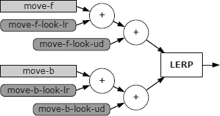
This corresponds to the tree shown in Figure 12.57.
Rapid Iteration
Naughty Dog’s animation team achieves rapid iteration with the help of four important tools:
12.10.3.2 Example: Unreal Engine 4
Unreal Engine 4 (UE4) provides its users with five tools for working with skeletal animations and skeletal meshes: The Skeleton Editor, the Skeletal Mesh Editor, the Animation Editor, the Animation Blueprint Editor, and the Physics Editor.
A complete discussion of Unreal Engine’s animation tools is beyond our scope here, but you can read more about it by searching for “Unreal Skeletal Mesh Animation System” online.
12.10.4 Transitions
To create a high-quality animating character, we must carefully manage the transitions between states in the action state machine to ensure that the splices between animations do not have a jarring and unpolished appearance. Most modern animation engines provide a data-driven mechanism for specifying exactly how transitions should be handled. In this section, we’ll explore how this mechanism works.
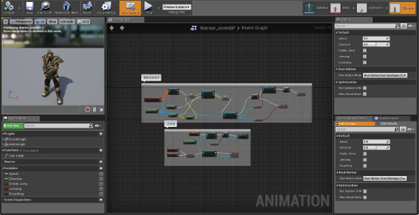
12.10.4.1 Kinds of Transitions
There are many different ways to manage the transition between states. If we know that the final pose of the source state exactly matches the first pose of the destination state, we can simply “pop” from one state to another. Otherwise, we can cross-fade from one state to the next. Cross-fading is not always a suitable choice when transitioning from state to state. For example, there is no way that a cross-fade can produce a realistic transition from lying on the ground to standing upright. For this kind of state transition, we need one or more custom animations. This kind of transition is often implemented by introducing special transitional states into the state machine. These states are intended for use only when going from one state to another—they are never used as a steady-state node. But because they are full-fledged states, they can be comprised of arbitrarily complex blend trees. This provides maximum flexibility when authoring custom-animated transitions.
12.10.4.2 Transition Parameters
When describing a particular transition between two states, we generally need to specify various parameters, controlling exactly how the transition will occur. These include but are not limited to the following.
12.10.4.3 The Transition Matrix
Specifying transitions between states can be challenging, because the number of possible transitions is usually very large. In a state machine with n states, the worst-case number of possible transitions is n2. We can imagine a two-dimensional square matrix with every possible state listed along both the vertical and horizontal axes. Such a table can be used to specify all of the possible transitions from any state along the vertical axis to any other state along the horizontal axis.
In a real game, this transition matrix is usually quite sparse, because not all state-to-state transitions are possible. For example, transitions are usually disallowed from a death state to any other state. Likewise, there is probably no way to go from a driving state to a swimming state (without going through at least one intermediate state that causes the character to jump out of his vehicle). The number of unique transitions in the table may be significantly less even than the number of valid transitions between states. This is because we can often reuse a single transition specification between many different pairs of states.
12.10.4.4 Implementing a Transition Matrix
There are all sorts of ways to implement a transition matrix. We could use a spreadsheet application to tabulate all the transitions in matrix form, or we might permit transitions to be authored in the same text file used to author our action states. If a graphical user interface is provided for state editing, transitions could be added to this GUI as well. In the following sections, we’ll take a brief look at a few transition matrix implementations from real game engines.
Example: Wildcarded Transitions in Medal of Honor: Pacific Assault
On Medal of Honor: Pacific Assault (MOHPA), we used the sparseness of the transition matrix to our advantage by supporting wildcarded transition specifications. For each transition specification, the names of both the source and destination states could contain asterisks (*) as a wildcard character. This allowed us to specify a single default transition from any state to any other state (via the syntax from=“*” to=“*”) and then refine this global default easily for entire categories of states. The refinement could be taken all the way down to custom transitions between specific state pairs when necessary. The MOHPA transition matrix looked something like this:
<transitions>
 <!-- global default -->
 <trans from=“*” to=“*”
  type=frozen duration=0.2>
 <!-- default for any walk to any run -->
 <trans from=“walk*” to=“run*”
  type=smooth
  duration=0.15>
<!-- special handling from any prone to any getting-up
 - - action (only valid from 2 sec to 7.5 sec on the
 - - local timeline) -- >
 <trans from=“*prone” to=“*get-up”
  type=smooth
  duration=0.1
  window-start=2.0
  window-end=7.5>
  …
 </transitions>
Example: First-Class Transitions in Uncharted
In some animation engines, high-level game code requests transitions from the current state to a new state by naming the destination state explicitly. The problem with this approach is that the calling code must have intimate knowledge of the names of the states and of which transitions are valid when in a particular state.
In Naughty Dog’s engine, this problem is overcome by turning state transitions from secondary implementation details into first-class entities. Each state provides a list of valid transitions to other states, and each transition is given a unique name. The names of the transitions are standardized in order to make the effect of each transition predictable. For example, if a transition is called “walk,” then it always goes from the current state to a walking state of some kind, no matter what the current state is. Whenever the high-level animation control code wants to transition from state A to state B, it asks for a transition by name (rather than requesting the destination state explicitly). If such a transition can be found and is valid, it is taken; otherwise, the request fails.
The following example state defines four transitions named “reload,” “step-left,” “step-right” and “fire.” The (transition-group …) line invokes a previously defined group of transitions; it is useful when the same set of transitions is to be used in multiple states. The (transition-end …) command specifies a transition that is taken upon reaching the end of the state’s local timeline if no other transition has been taken before then.
(define-state complex
 :name “s_turret-idle”
 :tree (aim-tree
  (anim-node-clip “turret-aim-all--base”)
  “turret-aim-all--left-right”
  “turret-aim-all--up-down”
 )
 :transitions (
 (transition “reload” “s_turret-reload”
  (range - -) :fade-time 0.2)
 (transition “step-left” “s_turret-step-left”
  (range - -) :fade-time 0.2)
 (transition “step-right” “s_turret-step-right”
  (range - -) :fade-time 0.2)
 (transition “fire” “s_turret-fire”
  (range - -) :fade-time 0.1)
 (transition-group “combat-gunout-idle^move”)
 (transition-end “s_turret-idle”)
 )
)
The beauty of this approach may be difficult to see at first. Its primary purpose is to allow transitions and states to be modified in a data-driven manner, without requiring changes to the C++ source code in many cases. This degree of flexibility is accomplished by shielding the animation control code from knowledge of the structure of the state graph. For example, let’s say that we have ten different walking states (normal, scared, crouched, injured and so on). All of them can transition into a jumping state, but different kinds of walks might require different jump animations (e.g., normal jump, scared jump, jump from crouch, injured jump, etc.). For each of the ten walking states, we define a transition simply called “jump.” At first, we can point all of these transitions to a single generic “jump” state, just to get things up and running. Later, we can fine-tune some of these transitions so that they point to custom jump states. We can even introduce transitional states between some of the “walk” states and their corresponding “jump” states. All sorts of changes can be made to the structure of the state graph and the parameters of the transitions without affecting the C++ source code—as long as the names of the transitions don’t change.
12.10.5 Control Parameters
From a software engineering perspective, it can be challenging to orchestrate all of the blend weights, playback rates and other control parameters of a complex animating character. Different blend weights have different effects on the way the character animates. For example, one weight might control the character’s movement direction, while others control its movement speed, horizontal and vertical weapon aim, head/eye look direction and so on. We need some way of exposing all of these blend weights to the code that is responsible for controlling them.
In a flat weighted average architecture, we have a flat list of all the animation clips that could possibly be played on the character. Each clip state has a blend weight, a playback rate and possibly other control parameters. The code that controls the character must look up individual clip states by name and adjust each one’s blend weight appropriately. This makes for a simple interface, but it shifts most of the responsibility for controlling the blend weights to the character control system. For example, to adjust the direction in which a character is running, the character control code must know that the “run” action is comprised of a group of animation clips, named something like “StrafeLeft,” “RunForward,” “StrafeRight” and “RunBackward.” It must look up these clip states by name and manually control all four blend weights in order to achieve a particular angled run animation. Needless to say, controlling animation parameters in such a fine-grained way can be tedious and can lead to difficult-to-understand source code.
In a blend tree, a different set of problems arise. Thanks to the tree structure, the clips are grouped naturally into functional units. Custom tree nodes can encapsulate complex character motions. These are both helpful advantages over the flat weighted average approach. However, the control parameters are buried within the tree. Code that wishes to control the horizontal look-at direction of the head and eyes needs a priori knowledge of the structure of the blend tree so that it can find the appropriate nodes in the tree in order to control their parameters.
Different animation engines solve these problems in different ways. Here are some examples:
Of course, there are many other alternatives as well. Every animation engine tackles this problem in a slightly different way, but the net effect is always roughly the same.
12.11 Constraints
We’ve seen how action state machines can be used to specify complex blend trees and how a transition matrix can be used to control how transitions between states should work. Another important aspect of character animation control is to constrain the movement of the characters and/or objects in the scene in various ways. For example, we might want to constrain a weapon so that it always appears to be in the hand of the character who is carrying it. We might wish to constrain two characters so that they line up properly when shaking hands. A character’s feet are often constrained so that they line up with the floor, and its hands might be constrained to line up with the rungs on a ladder or the steering wheel of a vehicle. In this section, we’ll take a brief look at how these constraints are handled in a typical animation system.

12.11.1 Attachments
Virtually all modern game engines permit objects to be attached to one another. At its simplest, object-to-object attachment involves constraining the position and/or orientation of a particular joint JA within the skeleton of object A so that it coincides with a joint JB in the skeleton of object B. An attachment is usually a parent-child relationship. When the parent’s skeleton moves, the child object is adjusted to satisfy the constraint. However, when the child moves, the parent’s skeleton is usually not affected. This is illustrated in Figure 12.59.
Sometimes it can be convenient to introduce an offset between the parent joint and the child joint. For example, when placing a gun into a character’s hand, we could constrain the “Grip” joint of the gun so that it coincides with the “RightWrist” joint of the character. However, this might not produce the correct alignment of the gun with the hand. One solution to this problem is to introduce a special joint into one of the two skeletons. For example, we could add a “RightGun” joint to the character’s skeleton, make it a child of the “RightWrist” joint, and position it so that when the “Grip” joint of the gun is constrained to it, the gun looks like it is being held naturally by the character. The problem with this approach, however, is that it increases the number of joints in the skeleton. Each joint has a processing cost associated with animation blending and matrix palette calculation and a memory cost for storing its animation keys. So adding new joints is often not a viable option.
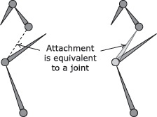
We know that an additional joint added for attachment purposes will not contribute to the pose of the character—it merely introduces an additional transform between the parent and child joint in an attachment. What we really want, then, is a way to mark certain joints so that they can be ignored by the animation blending pipeline but can still be used for attachment purposes. Such special joints are sometimes called attach points. They are illustrated in Figure 12.60.
Attach points might be modeled in Maya just like regular joints or locators, although many game engines define attach points in a more convenient manner. For example, they might be specified as part of the action state machine text file or via a custom GUI within the animation authoring tool. This allows the animators to focus only on the joints that affect the look of the character, while the power to control attachments is put conveniently into the hands of the people who need it—the game designers and the engineers.
12.11.2 Interobject Registration
The interactions between game characters and their environments is growing ever more complex and nuanced with each new title. Hence, it is important to have a system that allows characters and objects to be aligned with one another when animating. Such a system can be used for in-game cinematics and interactive gameplay elements alike.
Imagine that an animator, working in Maya or some other animation tool, sets up a scene involving two characters and a door object. The two characters shake hands, and then one of them opens the door and they both walk through it. The animator can ensure that all three actors in the scene line up perfectly. However, when the animations are exported, they become three separate clips, to be played on three separate objects in the game world. The two characters might have been under AI or player control prior to the start of this animated sequence. How, then, can we ensure that the three objects line up correctly with one another when the three clips are played back in-game?
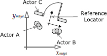

12.11.2.1 Reference Locators
One good solution is to introduce a common reference point into all three animation clips. In Maya, the animator can drop a locator (which is just a 3D transform, much like a skeletal joint) into the scene, placing it anywhere that seems convenient. Its location and orientation are actually irrelevant, as we’ll see. The locator is tagged in some way to tell the animation export tools that it is to be treated specially.
When the three animation clips are exported, the tools store the position and orientation of the reference locator, expressed in coordinates that are relative to the local object space of each actor, into all three clip’s data files. Later, when the three clips are played back in-game, the animation engine can look up the relative position and orientation of the reference locator in all three clips. It can then transform the origins of the three objects in such a way as to make all three reference locators coincide in world space. The reference locator acts much like an attach point (Section 12.11.1) and, in fact, could be implemented as one. The net effect—all three actors now line up with one another, exactly as they had been aligned in the original Maya scene.
Figure 12.61 illustrates how the door and the two characters from the above example might be set up in a Maya scene. As shown in Figure 12.62, the reference locator appears in each exported animation clip (expressed in that actor’s local space). In-game, these local-space reference locators are aligned to a fixed world-space locator in order to realign the actors, as shown in Figure 12.63.
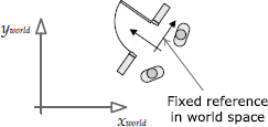
12.11.2.2 Finding the World-Space Reference Location
We’ve glossed over one important detail here—who decides what the world-space position and orientation of the reference locator should be? Each animation clip provides the reference locator’s transform in the coordinate space of its actor. But we need some way to define where that reference locator should be in world space.
In our example with the door and the two characters shaking hands, one of the actors is fixed in the world (the door). So one viable solution is to ask the door for the location of the reference locator and then align the two characters to it. The commands to accomplish this might look similar to the following pseudocode.
void playShakingHandsDoorSequence(
 Actor& door,
 Actor& characterA,
 Actor& characterB)
{
 // Find the world-space transform of the reference
 // locator as specified in the door’s animation.
 Transform refLoc = getReferenceLocatorWs(door,
  “shake-hands-door”);
 // Play the door’s animation in-place. (It’s
 // already in the correct place.)
 playAnimation(“shake-hands-door”, door);
 // Play the two characters’ animations relative to
 // the world-space reference locator obtained from
 // the door.
 playAnimationRelativeToReference(
 “shake-hands-character-a”, characterA, refLoc);
 playAnimationRelativeToReference(
 “shake-hands-character-b”, characterB, refLoc);
}
Another option is to define the world-space transform of the reference locator independently of the three actors in the scene. We could place the reference locator into the world using our world-building tool, for example (see Section 15.3). In this case, the pseudocode above should be changed to look something like this:
void playShakingHandsDoorSequence(
 Actor& door,
 Actor& characterA,
 Actor& characterB,
 Actor& refLocatorActor)
{
 // Find the world-space transform of the reference
 // locator by simply querying the transform of an
 // independent actor (presumably placed into the
 // world manually).
 Transform refLoc = getActorTransformWs(
  refLocatorActor);
 // Play all animations relative to the world-space
 // reference locator obtained above.
 playAnimationRelativeToReference(“shake-hands-door”,
  door, refLoc);
 playAnimationRelativeToReference(
  “shake-hands-character-a”, characterA, refLoc);
 playAnimationRelativeToReference(
  “shake-hands-character-b”, characterB, refLoc);
}
12.11.3 Grabbing and Hand IK
Even after using an attachment to connect two objects, we sometimes find that the alignment does not look exactly right in-game. For example, a character might be holding a rifle in her right hand, with her left hand supporting the stock. As the character aims the weapon in various directions, we may notice that the left hand no longer aligns properly with the stock at certain aim angles. This kind of joint misalignment is caused by LERP blending. Even if the joints in question are aligned perfectly in clip A and in clip B, LERP blending does not guarantee that those joints will be in alignment when A and B are blended together.
One solution to this problem is to use inverse kinematics (IK) to correct the position of the left hand. The basic approach is to determine the desired target position for the joint in question. IK is then applied to a short chain of joints (usually two, three or four joints), starting with the joint in question and progressing up the hierarchy to its parent, grandparent and so on. The joint whose position we are trying to correct is known as the end effector. The IK solver adjusts the orientations of the end effector’s parent joint(s) in order to get the end effector as close as possible to the target.
The API for an IK system usually takes the form of a request to enable or disable IK on a particular chain of joints, plus a specification of the desired target point. The actual IK calculation is usually done internally by the low-level animation pipeline. This allows it to do the calculation at the proper time—namely, after intermediate local and global skeletal poses have been calculated but before the final matrix palette calculation.
Some animation engines allow IK chains to be defined a priori. For example, we might define one IK chain for the left arm, one for the right arm and two for the two legs. Let’s assume for the purposes of this example that a particular IK chain is identified by the name of its end-effector joint. (Other engines might use an index or handle or some other unique identifier, but the concept remains the same.) The function to enable an IK calculation might look something like this:
void enableIkChain(Actor& actor,
  const char* endEffectorJointName,
  const Vector3& targetLocationWs);
and the function to disable an IK chain might look like this:
void disableIkChain(Actor& actor,
  const char* endEffectorJointName);
IK is usually enabled and disabled relatively infrequently, but the world-space target location must be kept up-to-date every frame (if the target is moving). Therefore, the low-level animation pipeline always provides some mechanism for updating an active IK target point. For example, the pipeline might allow us to call enableIkChain() multiple times. The first time it is called, the IK chain is enabled, and its target point is set. All subsequent calls simply update the target point. Another way to keep IK targets up-to-date is to link them to dynamic objects in the game. For example, an IK target might be specified as a handle to a rigid game object, or a joint within an animated object.
IK is well-suited to making minor corrections to joint alignment when the joint is already reasonably close to its target. It does not work nearly as well when the error between a joint’s desired location and its actual location is large. Note also that most IK algorithms solve only for the position of a joint. You may need to write additional code to ensure that the orientation of the end effector aligns properly with its target as well. IK is not a cure-all, and it may have significant performance costs. So always use it judiciously.

12.11.4 Motion Extraction and Foot IK
In games, we usually want the locomotion animations of our characters to look realistic and “grounded.” One of the biggest factors contributing to the realism of a locomotion animation is whether or not the feet slide around on the ground. Foot sliding can be overcome in a number of ways, the most common of which are motion extraction and foot IK.
12.11.4.1 Motion Extraction
Let’s imagine how we’d animate a character walking forward in a straight line. In Maya (or his or her animation package of choice), the animator makes the character take one complete step forward, first with the left foot and then with the right foot. The resulting animation clip is known as a locomotion cycle, because it is intended to be looped indefinitely, for as long as the character is walking forward in-game. The animator takes care to ensure that the feet of the character appear grounded and don’t slide as it moves. The character moves from its initial location on frame 0 to a new location at the end of the cycle. This is shown in Figure 12.64.
Notice that the local-space origin of the character remains fixed during the entire walk cycle. In effect, the character is “leaving his origin behind him” as he takes his step forward. Now imagine playing this animation as a loop. We would see the character take one complete step forward, and then pop back to where he was on the first frame of the animation. Clearly this won’t work in-game.

To make this work, we need to remove the forward motion of the character, so that his local-space origin remains roughly under the center of mass of the character at all times. We could do this by zeroing out the forward translation of the root joint of the character’s skeleton. The resulting animation clip would make the character look like he’s “moonwalking,” as shown in Figure 12.65.
In order to get the feet to appear to “stick” to the ground the way they did in the original Maya scene, we need the character to move forward by just the right amount each frame. We could look at the distance the character moved, divide by the amount of time it took for him to get there, and hence find his average movement speed. But a character’s forward speed is not constant when walking. This is especially evident when a character is limping (quick forward motion on the injured leg, followed by slower motion on the “good” leg), but it is true for all natural-looking walk cycles.
Therefore, before we zero out the forward motion of the root joint, we first save the animation data in a special “extracted motion” channel. This data can be used in-game to move the local-space origin of the character forward by the exact amount that the root joint had moved in Maya each frame. The net result is that the character will walk forward exactly as he was authored, but now his local-space origin comes along for the ride, allowing the animation to loop properly. This is shown in Figure 12.66.
If the character moves forward by 4 feet in the animation and the animation takes one second to complete, then we know that the character is moving at an average speed of 4 feet/second. To make the character walk at a different speed, we can simply scale the playback rate of the walk cycle animation. For example, to make the character walk at 2 feet/second, we can simply play the animation at half speed (R = 0.5).
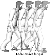
12.11.4.2 Foot IK
Motion extraction does a good job of making a character’s feet appear grounded when it is moving in a straight line (or, more correctly, when it moves in a path that exactly matches the path animated by the animator). However, a real game character must be turned and moved in ways that don’t coincide with the original hand-animated path of motion (e.g., when moving over uneven terrain). This results in additional foot sliding.
One solution to this problem is to use IK to correct for any sliding in the feet. The basic idea is to analyze the animations to determine during which periods of time each foot is fully in contact with the ground. At the moment a foot contacts the ground, we note its world-space location. For all subsequent frames while that foot remains on the ground, we use IK to adjust the pose of the leg so that the foot remains fixed to the proper location. This technique sounds easy enough, but getting it to look and feel right can be very challenging. It requires a lot of iteration and fine-tuning. And some natural human motions—like leading into a turn by increasing your stride—cannot be produced by IK alone.
In addition, there is a big trade-off between the look of the animations and the feel of the character, particularly for a human-controlled character. It’s generally more important for the player character control system to feel responsive and fun than it is for the character’s animations to look perfect. The upshot is this: Do not take the task of adding foot IK or motion extraction to your game lightly. Budget time for a lot of trial and error, and be prepared to make tradeoffs to ensure that your player character not only looks good but feels good as well.
12.11.5 Other Kinds of Constraints
There are plenty of other possible kinds of constraint systems that can be added to a game animation engine. Some examples include: