
11
The Rendering Engine
When most people think about computer and video games, the first thing that comes to mind is the stunning three-dimensional graphics. Realtime 3D rendering is an exceptionally broad and profound topic, so there’s simply no way to cover all of the details in a single chapter. Thankfully there are a great many excellent books and other resources available on this topic. In fact, real-time 3D graphics is perhaps one of the best covered of all the technologies that make up a game engine. The goal of this chapter, then, is to provide you with a broad understanding of real-time rendering technology and to serve as a jumping-off point for further learning. After you’ve read through these pages, you should find that reading other books on 3D graphics seems like a journey through familiar territory. You might even be able to impress your friends at parties (…or alienate them…).
We’ll begin by laying a solid foundation in the concepts, theory and mathematics that underlie any real-time 3D rendering engine. Next, we’ll have a look at the software and hardware pipelines used to turn this theoretical framework into reality. We’ll discuss some of the most common optimization techniques and see how they drive the structure of the tools pipeline and the runtime rendering API in most engines. We’ll end with a survey of some of the advanced rendering techniques and lighting models in use by game engines today. Throughout this chapter, I’ll point you to some of my favorite books and other resources that should help you to gain an even deeper understanding of the topics we’ll cover here.
11.1 Foundations of Depth-Buffered Triangle Rasterization
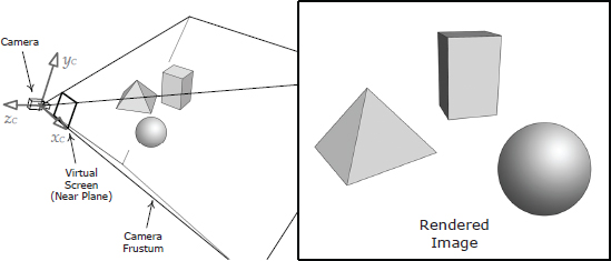
When you boil it down to its essence, rendering a three-dimensional scene involves the following basic steps:
This high-level rendering process is depicted in Figure 11.1.
Many different technologies can be used to perform the basic rendering steps described above. The primary goal is usually photorealism, although some games aim for a more stylized look (e.g., cartoon, charcoal sketch, watercolor and so on). As such, rendering engineers and artists usually attempt to describe the properties of their scenes as realistically as possible and to use light transport models that match physical reality as closely as possible. Within this context, the gamut of rendering technologies ranges from techniques designed for real-time performance at the expense of visual fidelity, to those designed for photorealism but which are not intended to operate in real time.
Real-time rendering engines perform the steps listed above repeatedly, displaying rendered images at a rate of 30, 50 or 60 frames per second to provide the illusion of motion. This means a real-time rendering engine has at most 33.3 ms to generate each image (to achieve a frame rate of 30 FPS). Usually much less time is available, because bandwidth is also consumed by other engine systems like animation, AI, collision detection, physics simulation, audio, player mechanics and other gameplay logic. Considering that film rendering engines often take anywhere from many minutes to many hours to render a single frame, the quality of real-time computer graphics these days is truly astounding.
11.1.1 Describing a Scene
A real-world scene is composed of objects. Some objects are solid, like a brick, and some are amorphous, like a cloud of smoke, but every object occupies a volume of 3D space. An object might be opaque (in which case light cannot pass through its volume), transparent (in which case light passes through it without being scattered, so that we can see a reasonably clear image of whatever is behind the object), or translucent (meaning that light can pass through the object but is scattered in all directions in the process, yielding only a blur of colors that hint at the objects behind it).
Opaque objects can be rendered by considering only their surfaces. We don’t need to know what’s inside an opaque object in order to render it, because light cannot penetrate its surface. When rendering a transparent or translucent object, we really should model how light is reflected, refracted, scattered and absorbed as it passes through the object’s volume. This requires knowledge of the interior structure and properties of the object. However, most game engines don’t go to all that trouble. They just render the surfaces of transparent and translucent objects in almost the same way opaque objects are rendered. A simple numeric opacity measure known as alpha is used to describe how opaque or transparent a surface is. This approach can lead to various visual anomalies (for example, surface features on the far side of the object may be rendered incorrectly), but the approximation can be made to look reasonably realistic in many cases. Even amorphous objects like clouds of smoke are often represented using particle effects, which are typically composed of large numbers of semitransparent rectangular cards. Therefore, it’s safe to say that most game rendering engines are primarily concerned with rendering surfaces.
11.1.1.1 Representations Used by High-End Rendering Packages
Theoretically, a surface is a two-dimensional sheet comprised of an infinite number of points in three-dimensional space. However, such a description is clearly not practical. In order for a computer to process and render arbitrary surfaces, we need a compact way to represent them numerically.
Some surfaces can be described exactly in analytical form using a parametric surface equation. For example, a sphere centered at the origin can be represented by the equation x2 + y2 + z2 = r2. However, parametric equations aren’t particularly useful for modeling arbitrary shapes.
In the film industry, surfaces are often represented by a collection of rectangular patches each formed from a two-dimensional spline defined by a small number of control points. Various kinds of splines are used, including Bézier surfaces (e.g., bicubic patches, which are third-order Béziers—see http://en.wikipedia.org/wiki/Bezier_surface for more information), nonuniform rational B-splines (NURBS—see http://en.wikipedia.org/wiki/Nurbs), Bézier triangles and N-patches (also known as normal patches—see http://ubm.io/1iGnvJ5 for more details). Modeling with patches is a bit like covering a statue with little rectangles of cloth or paper maché.
High-end film rendering engines like Pixar’s RenderMan use subdivision surfaces to define geometric shapes. Each surface is represented by a mesh of control polygons (much like a spline), but the polygons can be subdivided into smaller and smaller polygons using the Catmull-Clark algorithm. This subdivision typically proceeds until the individual polygons are smaller than a single pixel in size. The biggest benefit of this approach is that no matter how close the camera gets to the surface, it can always be subdivided further so that its silhouette edges won’t look faceted. To learn more about subdivision surfaces, check out the following great article: http://ubm.io/1lx6th5.
11.1.1.2 Triangle Meshes
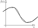
Game developers have traditionally modeled their surfaces using triangle meshes. Triangles serve as a piecewise linear approximation to a surface, much as a chain of connected line segments acts as a piecewise approximation to a function or curve (see Figure 11.2).
Triangles are the polygon of choice for real-time rendering because they have the following desirable properties:
Tessellation
The term tessellation describes a process of dividing a surface up into a collection of discrete polygons (which are usually either quadrilaterals, also known as quads, or triangles). Triangulation is tessellation of a surface into triangles.
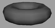
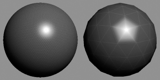
One problem with the kind of triangle mesh used in games is that its level of tessellation is fixed by the artist when he or she creates it. Fixed tessellation can cause an object’s silhouette edges to look blocky, as shown in Figure 11.3; this is especially noticeable when the object is close to the camera.
Ideally, we’d like a solution that can arbitrarily increase tessellation as an object gets closer to the virtual camera. In other words, we’d like to have a uniform triangle-to-pixel density, no matter how close or far away the object is. Subdivision surfaces can achieve this ideal—surfaces can be tessellated based on distance from the camera, so that every triangle is less than one pixel in size.
Game developers often attempt to approximate this ideal of uniform triangle-to-pixel density by creating a chain of alternate versions of each triangle mesh, each known as a level of detail (LOD). The first LOD, often called LOD 0, represents the highest level of tessellation; it is used when the object is very close to the camera. Subsequent LODs are tessellated at lower and lower resolutions (see Figure 11.4). As the object moves farther away from the camera, the engine switches from LOD 0 to LOD 1 to LOD 2 and so on. This allows the rendering engine to spend the majority of its time transforming and lighting the vertices of the objects that are closest to the camera (and therefore occupy the largest number of pixels on-screen).
Some game engines apply dynamic tessellation techniques to expansive meshes like water or terrain. In this technique, the mesh is usually represented by a height field defined on some kind of regular grid pattern. The region of the mesh that is closest to the camera is tessellated to the full resolution of the grid. Regions that are farther away from the camera are tessellated using fewer and fewer grid points.
Progressive meshes are another technique for dynamic tessellation and LODing. With this technique, a single high-resolution mesh is created for display when the object is very close to the camera. (This is essentially the LOD 0 mesh.) This mesh is automatically detessellated as the object gets farther away by collapsing certain edges. In effect, this process automatically generates a semi-continuous chain of LODs. See http://research.microsoft.com/en-us/um/people/hoppe/pm.pdf for a detailed discussion of progressive mesh technology.

11.1.1.3 Constructing a Triangle Mesh
Now that we understand what triangle meshes are and why they’re used, let’s take a brief look at how they’re constructed.
Winding Order
A triangle is defined by the position vectors of its three vertices, which we can denote p1, p2 and p3. The edges of a triangle can be found by simply subtracting the position vectors of adjacent vertices. For example,
The normalized cross product of any two edges defines a unit face normal N:
These derivations are illustrated in Figure 11.5. To know the direction of the face normal (i.e., the sense of the edge cross product), we need to define which side of the triangle should be considered the front (i.e., the outside surface of an object) and which should be the back (i.e., its inside surface). This can be defined easily by specifying a winding order—clockwise (CW) or counterclockwise (CCW).
Most low-level graphics APIs give us a way to cull back-facing triangles based on winding order. For example, if we set the cull mode parameter in Direct3D (D3DRS_CULL) to D3DCULLMODE_CW, then any triangle whose vertices wind in a clockwise fashion in screen space will be treated as a back-facing triangle and will not be drawn.

Back-face culling is important because we generally don’t want to waste time drawing triangles that aren’t going to be visible anyway. Also, rendering the back faces of transparent objects can actually cause visual anomalies. The choice of winding order is an arbitrary one, but of course it must be consistent across all assets in the entire game. Inconsistent winding order is a common error among junior 3D modelers.
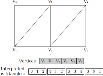
Triangle Lists
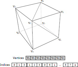
The easiest way to define a mesh is simply to list the vertices in groups of three, each triple corresponding to a single triangle. This data structure is known as a triangle list; it is illustrated in Figure 11.6.

Indexed Triangle Lists
You probably noticed that many of the vertices in the triangle list shown in Figure 11.6 were duplicated, often multiple times. As we’ll see in Section 11.1.2.1, we often store quite a lot of metadata with each vertex, so repeating this data in a triangle list wastes memory. It also wastes GPU bandwidth, because a duplicated vertex will be transformed and lit multiple times.
For these reasons, most rendering engines make use of a more efficient data structure known as an indexed triangle list. The basic idea is to list the vertices once with no duplication and then to use lightweight vertex indices (usually occupying only 16 bits each) to define the triples of vertices that constitute the triangles. The vertices are stored in an array known as a vertex buffer (DirectX) or vertex array (OpenGL). The indices are stored in a separate buffer known as an index buffer or index array. This technique is shown in Figure 11.7.
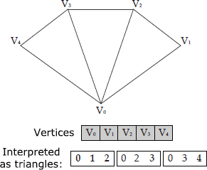
Strips and Fans
Specialized mesh data structures known as triangle strips and triangle fans are sometimes used for game rendering. Both of these data structures eliminate the need for an index buffer, while still reducing vertex duplication to some degree. They accomplish this by predefining the order in which vertices must appear and how they are combined to form triangles.
In a strip, the first three vertices define the first triangle. Each subsequent vertex forms an entirely new triangle, along with its previous two neighbors. To keep the winding order of a triangle strip consistent, the previous two neighbor vertices swap places after each new triangle. A triangle strip is shown in Figure 11.8.
In a fan, the first three vertices define the first triangle and each subsequent vertex defines a new triangle with the previous vertex and the first vertex in the fan. This is illustrated in Figure 11.9.
Vertex Cache Optimization
When a GPU processes an indexed triangle list, each triangle can refer to any vertex within the vertex buffer. The vertices must be processed in the order they appear within the triangles, because the integrity of each triangle must be maintained for the rasterization stage. As vertices are processed by the vertex shader, they are cached for reuse. If a subsequent primitive refers to a vertex that already resides in the cache, its processed attributes are used instead of reprocessing the vertex.
Strips and fans are used in part because they can potentially save memory (no index buffer required) and in part because they tend to improve the cache coherency of the memory accesses made by the GPU to video RAM. Even better, we can use an indexed strip or indexed fan to virtually eliminate vertex duplication (which can often save more memory than eliminating the index buffer), while still reaping the cache coherency benefits of the strip or fan vertex ordering.
Indexed triangle lists can also be cache-optimized without restricting ourselves to strip or fan vertex ordering. A vertex cache optimizer is an offline geometry processing tool that attempts to list the triangles in an order that optimizes vertex reuse within the cache. It generally takes into account factors such as the size of the vertex cache(s) present on a particular type of GPU and the algorithms used by the GPU to decide when to cache vertices and when to discard them. For example, the vertex cache optimizer included in Sony’s Edge geometry processing library can achieve rendering throughput that is up to 4% better than what is possible with triangle stripping.
11.1.1.4 Model Space
The position vectors of a triangle mesh’s vertices are usually specified relative to a convenient local coordinate system called model space, local space, or object space. The origin of model space is usually either in the center of the object or at some other convenient location, like on the floor between the feet of a character or on the ground at the horizontal centroid of the wheels of a vehicle.

As we learned in Section 5.3.9.1, the sense of the model-space axes is arbitrary, but the axes typically align with the natural “front,” “left,” “right” and “up” directions on the model. For a little mathematical rigor, we can define three unit vectors F, L (or R) and U and map them as desired onto the unit basis vectors i, j and k (and hence to the x-, y- and z-axes, respectively) in model space. For example, a common mapping is L = i, U = j and F = k. The mapping is completely arbitrary, but it’s important to be consistent for all models across the entire engine. Figure 11.10 shows one possible mapping of the model-space axes for an aircraft model.
11.1.1.5 World Space and Mesh Instancing
Many individual meshes are composed into a complete scene by positioning and orienting them within a common coordinate system known as world space. Any one mesh might appear many times in a scene—examples include a street lined with identical lamp posts, a faceless mob of soldiers or a swarm of spiders attacking the player. We call each such object a mesh instance.
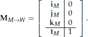
A mesh instance contains a reference to its shared mesh data and also includes a transformation matrix that converts the mesh’s vertices from model space to world space, within the context of that particular instance. This matrix is called the model-to-world matrix, or sometimes just the world matrix. Using the notation from Section 5.3.10.2, this matrix can be written as follows:
where the upper 3 × 3 matrix (RS)M→W rotates and scales model-space vertices into world space, and tM is the translation of the model-space axes expressed in world space. If we have the unit model-space basis vectors iM, jMand kM, expressed in world-space coordinates, this matrix can also be written as follows:
Given a vertex expressed in model-space coordinates, the rendering engine calculates its world-space equivalent as follows:
We can think of the matrix MM→W as a description of the position and orientation of the model-space axes themselves, expressed in world-space coordinates. Or we can think of it as a matrix that transforms vertices from model space to world space.
When rendering a mesh, the model-to-world matrix is also applied to the surface normals of the mesh (see Section 11.1.2.1). Recall from Section 5.3.11, that in order to transform normal vectors properly, we must multiply them by the inverse transpose of the model-to-world matrix. If our matrix does not contain any scale or shear, we can transform our normal vectors correctly by simply setting their w components to zero prior to multiplication by the model-to-world matrix, as described in Section 5.3.6.1.
Some meshes like buildings, terrain and other background elements are entirely static and unique. The vertices of these meshes are often expressed in world space, so their model-to-world matrices are identity and can be ignored.
11.1.2 Describing the Visual Properties of a Surface
In order to properly render and light a surface, we need a description of its visual properties. Surface properties include geometric information, such as the direction of the surface normal at various points on the surface. They also encompass a description of how light should interact with the surface. This includes diffuse color, shininess/reflectivity, roughness or texture, degree of opacity or transparency, index of refraction and other optical properties. Surface properties might also include a specification of how the surface should change over time (e.g., how an animated character’s skin should track the joints of its skeleton or how the surface of a body of water should move).
The key to rendering photorealistic images is properly accounting for light’s behavior as it interacts with the objects in the scene. Hence rendering engineers need to have a good understanding of how light works, how it is transported through an environment and how the virtual camera “senses” it and translates it into the colors stored in the pixels on-screen.
11.1.2.1 Introduction to Light and Color
Light is electromagnetic radiation; it acts like both a wave and a particle in different situations. The color of light is determined by its intensity I and its wavelength λ (or its frequency f, where f = 1/λ). The visible gamut ranges from a wavelength of 740 nm (or a frequency of 430 THz) to a wavelength of 380 nm (750 THz). A beam of light may contain a single pure wavelength (i.e., the colors of the rainbow, also known as the spectral colors), or it may contain a mixture of various wavelengths. We can draw a graph showing how much of each frequency a given beam of light contains, called a spectral plot. White light contains a little bit of all wavelengths, so its spectral plot would look roughly like a box extending across the entire visible band. Pure green light contains only one wavelength, so its spectral plot would look like a single infinitesimally narrow spike at about 570 THz.
Light-Object Interactions
Light can have many complex interactions with matter. Its behavior is governed in part by the medium through which it is traveling and in part by the shape and properties of the interfaces between different types of media (airsolid, air-water, water-glass, etc.). Technically speaking, a surface is really just an interface between two different types of media.
Despite all of its complexity, light can really only do four things:
Most photorealistic rendering engines account for the first three of these behaviors; diffraction is not usually taken into account because its effects are rarely noticeable in most scenes.
Only certain wavelengths may be absorbed by a surface, while others are reflected. This is what gives rise to our perception of the color of an object. For example, when white light falls on a red object, all wavelengths except red are absorbed, hence the object appears red. The same perceptual effect is achieved when red light is cast onto a white object—our eyes don’t know the difference.
Reflections can be diffuse, meaning that an incoming ray is scattered equally in all directions. Reflections can also be specular, meaning that an incident light ray will reflect directly or be spread only into a narrow cone. Reflections can also be anisotropic, meaning that the way in which light reflects from a surface changes depending on the angle at which the surface is viewed.
When light is transmitted through a volume, it can be scattered (as is the case for translucent objects), partially absorbed (as with colored glass), or refracted (as happens when light travels through a prism). The refraction angles can be different for different wavelengths, leading to spectral spreading. This is why we see rainbows when light passes through raindrops and glass prisms. Light can also enter a semi-solid surface, bounce around and then exit the surface at a different point from the one at which it entered the surface. We call this subsurface scattering, and it is one of the effects that gives skin, wax and marble their characteristic warm appearance.
Color Spaces and Color Models
A color model is a three-dimensional coordinate system that measures colors. A color space is a specific standard for how numerical colors in a particular color model should be mapped onto the colors perceived by human beings in the real world. Color models are typically three-dimensional because of the three types of color sensors (cones) in our eyes, which are sensitive to different wavelengths of light.
The most commonly used color model in computer graphics is the RGB model. In this model, color space is represented by a unit cube, with the relative intensities of red, green and blue light measured along its axes. The red, green and blue components are called color channels. In the canonical RGB color model, each channel ranges from zero to one. So the color (0, 0, 0) represents black, while (1, 1, 1) represents white.
When colors are stored in a bitmapped image, various color formats can be employed. A color format is defined in part by the number of bits per pixel it occupies and, more specifically, the number of bits used to represent each color channel. The RGB888 format uses eight bits per channel, for a total of 24 bits per pixel. In this format, each channel ranges from 0 to 255 rather than from zero to one. RGB565 uses five bits for red and blue and six for green, for a total of 16 bits per pixel. A paletted format might use eight bits per pixel to store indices into a 256-element color palette, each entry of which might be stored in RGB888 or some other suitable format.
A number of other color models are also used in 3D rendering. We’ll see how the log-LUV color model is used for high dynamic range (HDR) lighting in Section 11.3.1.5.
Opacity and the Alpha Channel
A fourth channel called alpha is often tacked on to RGB color vectors. As mentioned in Section 11.1.1, alpha measures the opacity of an object. When stored in an image pixel, alpha represents the opacity of the pixel.
RGB color formats can be extended to include an alpha channel, in which case they are referred to as RGBA or ARGB color formats. For example, RGBA8888 is a 32 bit-per-pixel format with eight bits each for red, green, blue and alpha. RGBA5551 is a 16 bit-per-pixel format with one-bit alpha; in this format, colors can either be fully opaque or fully transparent.
11.1.2.2 Vertex Attributes
The simplest way to describe the visual properties of a surface is to specify them at discrete points on the surface. The vertices of a mesh are a convenient place to store surface properties, in which case they are called vertex attributes.
A typical triangle mesh includes some or all of the following attributes at each vertex. As rendering engineers, we are of course free to define any additional attributes that may be required in order to achieve a desired visual effect on-screen.
11.1.2.3 Vertex Formats
Vertex attributes are typically stored within a data structure such as a C struct or a C++ class. The layout of such a data structure is known as a vertex format. Different meshes require different combinations of attributes and hence need different vertex formats. The following are some examples of common vertex formats:
// Simplest possible vertex -- position only (useful for
// shadow volume extrusion, silhouette edge detection
// for cartoon rendering, z-prepass, etc.)
struct Vertex1P
{
 Vector3 m_p; // position
};
// A typical vertex format with position, vertex normal
// and one set of texture coordinates.
struct Vertex1P1N1UV
{
 Vector3 m_p; // position
 Vector3 m_n; // vertex normal
 F32 m_uv[2]; // (u, v) texture coordinate
};
// A skinned vertex with position, diffuse and specular
// colors and four weighted joint influences.
struct Vertex1P1D1S2UV4J
{
 Vector3 m_p; // position
 Color4 m_d; // diffuse color and translucency
 Color4 m_S; // specular color
 F32 m_uv0[2]; // first set of tex coords
 F32 m_uv1[2]; // second set of tex coords
 U8 m_k[4]; // four joint indices, and…
 F32 m_w[3]; // three joint weights, for
 // skinning (fourth is calc’d
 // from the first three)
};
Clearly the number of possible permutations of vertex attributes—and hence the number of distinct vertex formats—can grow to be extremely large. (In fact the number of formats is theoretically unbounded, if one were to permit any number of texture coordinates and/or joint weights.) Management of all these vertex formats is a common source of headaches for any graphics programmer.
Some steps can be taken to reduce the number of vertex formats that an engine has to support. In practical graphics applications, many of the theoretically possible vertex formats are simply not useful, or they cannot be handled by the graphics hardware or the game’s shaders. Some game teams also limit themselves to a subset of the useful/feasible vertex formats in order to keep things more manageable. For example, they might only allow zero, two or four joint weights per vertex, or they might decide to support no more than two sets of texture coordinates per vertex. Some GPUs are capable of extracting a subset of attributes from a vertex data structure, so game teams can also choose to use a single “überformat” for all meshes and let the hardware select the relevant attributes based on the requirements of the shader.
11.1.2.4 Attribute Interpolation
The attributes at a triangle’s vertices are just a coarse, discretized approximation to the visual properties of the surface as a whole. When rendering a triangle, what really matters are the visual properties at the interior points of the triangle as “seen” through each pixel on-screen. In other words, we need to know the values of the attributes on a per-pixel basis, not a per-vertex basis.


One simple way to determine the per-pixel values of a mesh’s surface attributes is to linearly interpolate the per-vertex attribute data. When applied to vertex colors, attribute interpolation is known as Gouraud shading. An example of Gouraud shading applied to a triangle is shown in Figure 11.11, and its effects on a simple triangle mesh are illustrated in Figure 11.12. Interpolation is routinely applied to other kinds of vertex attribute information as well, such as vertex normals, texture coordinates and depth.
Vertex Normals and Smoothing
As we’ll see in Section 11.1.3, lighting is the process of calculating the color of an object at various points on its surface, based on the visual properties of the surface and the properties of the light impinging upon it. The simplest way to light a mesh is to calculate the color of the surface on a per-vertex basis. In other words, we use the properties of the surface and the incoming light to calculate the diffuse color of each vertex (di). These vertex colors are then interpolated across the triangles of the mesh via Gouraud shading.
In order to determine how a ray of light will reflect from a point on a surface, most lighting models make use of a vector that is normal to the surface at the point of the light ray’s impact. Since we’re performing lighting calculations on a per-vertex basis, we can use the vertex normal ni for this purpose. Therefore, the directions of a mesh’s vertex normals can have a significant impact on the final appearance of a mesh.
As an example, consider a tall, thin, four-sided box. If we want the box to appear to be sharp-edged, we can specify the vertex normals to be perpendicular to the faces of the box. As we light each triangle, we will encounter the same normal vector at all three vertices, so the resulting lighting will appear flat, and it will abruptly change at the corners of the box just as the vertex normals do.
We can also make the same box mesh look a bit like a smooth cylinder by specifying vertex normals that point radially outward from the box’s center line. In this case, the vertices of each triangle will have different vertex normals, causing us to calculate different colors at each vertex. Gouraud shading will smoothly interpolate these vertex colors, resulting in lighting that appears to vary smoothly across the surface. This effect is illustrated in Figure 11.13.
11.1.2.5 Textures
When triangles are relatively large, specifying surface properties on a pervertex basis can be too coarse-grained. Linear attribute interpolation isn’t always what we want, and it can lead to undesirable visual anomalies.
As an example, consider the problem of rendering the bright specular highlight that can occur when light shines on a glossy object. If the mesh is highly tessellated, per-vertex lighting combined with Gouraud shading can yield reasonably good results. However, when the triangles are too large, the errors that arise from linearly interpolating the specular highlight can become jarringly obvious, as shown in Figure 11.14.
To overcome the limitations of per-vertex surface attributes, rendering engineers use bitmapped images known as texture maps. A texture often contains color information and is usually projected onto the triangles of a mesh. In this case, it acts a bit like those silly fake tattoos we used to apply to our arms when we were kids. But a texture can contain other kinds of visual surface properties as well as colors. And a texture needn’t be projected onto a mesh—for example, a texture might be used as a stand-alone data table. The individual picture elements of a texture are called texels to differentiate them from the pixels on the screen.
The dimensions of a texture bitmap are constrained to be powers of two on some graphics hardware. Typical texture dimensions include 256 × 256, 512 × 512, 1024 × 1024 and 2048 × 2048, although textures can be any size on most hardware, provided the texture fits into video memory. Some graphics hardware imposes additional restrictions, such as requiring textures to be square, or lifts some restrictions, such as not constraining texture dimensions to be powers of two.
Types of Textures
The most common type of texture is known as a diffuse map, or albedo map. It describes the diffuse surface color at each texel on a surface and acts like a decal or paint job on the surface.
Other types of textures are used in computer graphics as well, including normal maps (which store unit normal vectors at each texel, encoded as RGB values), gloss maps (which encode how shiny a surface should be at each texel), environment maps (which contain a picture of the surrounding environment for rendering reflections) and many others. See Section 11.3.1 for a discussion of how various types of textures can be used for image-based lighting and other effects.
We can actually use texture maps to store any information that we happen to need in our lighting calculations. For example, a one-dimensional texture could be used to store sampled values of a complex math function, a color-to-color mapping table, or any other kind of look-up table (LUT).
Texture Coordinates
Let’s consider how to project a two-dimensional texture onto a mesh. To do this, we define a two-dimensional coordinate system known as texture space. A texture coordinate is usually represented by a normalized pair of numbers denoted (u, v). These coordinates always range from (0, 0) at the bottom left corner of the texture to (1, 1) at the top right. Using normalized coordinates like this allows the same coordinate system to be used regardless of the dimensions of the texture.
To map a triangle onto a 2D texture, we simply specify a pair of texture coordinates (ui,vi) at each vertex i. This effectively maps the triangle onto the image plane in texture space. An example of texture mapping is depicted in Figure 11.15.
Texture Addressing Modes
Texture coordinates are permitted to extend beyond the [0, 1] range. The graphics hardware can handle out-of-range texture coordinates in any one of the following ways. These are known as texture addressing modes; which mode is used is under the control of the user.

These texture addressing modes are depicted in Figure 11.16.
Texture Formats
Texture bitmaps can be stored on disk in virtually any image format, provided your game engine includes the code necessary to read it into memory. Common formats include Targa (.tga), Portable Network Graphics (.png), Windows Bitmap (.bmp) and Tagged Image File Format (.tif). In memory, textures are usually represented as two-dimensional (strided) arrays of pixels using various color formats, including RGB888, RGBA8888, RGB565, RGBA5551 and so on.
Most modern graphics cards and graphics APIs support compressed textures. DirectX supports a family of compressed formats known as DXT or S3 Texture Compression (S3TC). We won’t cover the details here, but the basic idea is to break the texture into 4 × 4 blocks of pixels and use a small color palette to store the colors for each block. You can read more about S3 compressed texture formats at http://en.wikipedia.org/wiki/S3_Texture_Compression.
Compressed textures have the obvious benefit of using less memory than their uncompressed counterparts. An additional unexpected plus is that they are faster to render with as well. S3 compressed textures achieve this speedup because of more cache-friendly memory access patterns—4 × 4 blocks of adjacent pixels are stored in a single 64- or 128-bit machine word—and because more of the texture can fit into the cache at once. Compressed textures do suffer from compression artifacts. While the anomalies are usually not noticeable, there are situations in which uncompressed textures must be used.
Texel Density and Mipmapping
Imagine rendering a full-screen quad (a rectangle composed of two triangles) that has been mapped with a texture whose resolution exactly matches that of the screen. In this case, each texel maps exactly to a single pixel on-screen, and we say that the texel density (ratio of texels to pixels) is one. When this same quad is viewed at a distance, its on-screen area becomes smaller. The resolution of the texture hasn’t changed, so the quad’s texel density is now greater than one (meaning that more than one texel is contributing to each pixel).
Clearly texel density is not a fixed quantity—it changes as a texture-mapped object moves relative to the camera. Texel density affects the memory consumption and the visual quality of a three-dimensional scene. When the texel density is much less than one, the texels become significantly larger than a pixel on-screen, and you can start to see the edges of the texels. This destroys the illusion. When texel density is much greater than one, many texels contribute to a single pixel on-screen. This can cause a moiré banding pattern, as shown in Figure 11.17. Worse, a pixel’s color can appear to swim and flicker as different texels within the boundaries of the pixel dominate its color depending on subtle changes in camera angle or position. Rendering a distant object with a very high texel density can also be a waste of memory if the player can never get close to it. After all, why keep such a high-res texture in memory if no one will ever see all that detail?
Ideally we’d like to maintain a texel density that is close to one at all times, for both nearby and distant objects. This is impossible to achieve exactly, but it can be approximated via a technique called mipmapping. For each texture, we create a sequence of lower-resolution bitmaps, each of which is one-half the width and one-half the height of its predecessor. We call each of these images a mipmap, or mip level. For example, a 64 × 64 texture would have the following mip levels: 64 × 64, 32 × 32, 16 × 16, 8 × 8, 4 × 4, 2 × 2 and 1 × 1, as shown in Figure 11.18. Once we have mipmapped our textures, the graphics hardware selects the appropriate mip level based on a triangle’s distance away from the camera, in an attempt to maintain a texel density that is close to one. For example, if a texture takes up an area of 40 × 40 on-screen, the 64 × 64 mip level might be selected; if that same texture takes up only a 10 × 10 area, the 16 × 16 mip level might be used. As we’ll see below, trilinear filtering allows the hardware to sample two adjacent mip levels and blend the results. In this case, a 10 × 10 area might be mapped by blending the 16 × 16 and 8 × 8 mip levels together.


World-Space Texel Density
The term “texel density” can also be used to describe the ratio of texels to world-space area on a textured surface. For example, a 2 m cube mapped with a 256 × 256 texture would have a texel density of 2562/22 = 16,384. I will call this world-space texel density to differentiate it from the screen-space texel density we’ve been discussing thus far.
World-space texel density need not be close to one, and in fact the specific value will usually be much greater than one and depends entirely upon your choice of world units. Nonetheless, it is important for objects to be texture mapped with a reasonably consistent world-space texel density. For example, we would expect all six sides of a cube to occupy the same texture area. If this were not the case, the texture on one side of the cube would have a lower-resolution appearance than another side, which can be noticeable to the player. Many game studios provide their art teams with guidelines and in-engine texel density visualization tools in an effort to ensure that all objects in the game have a reasonably consistent world-space texel density.
Texture Filtering
When rendering a pixel of a textured triangle, the graphics hardware samples the texture map by considering where the pixel center falls in texture space. There is usually not a clean one-to-one mapping between texels and pixels, and pixel centers can fall at any place in texture space, including directly on the boundary between two or more texels. Therefore, the graphics hardware usually has to sample more than one texel and blend the resulting colors to arrive at the actual sampled texel color. We call this texture filtering.
Most graphics cards support the following kinds of texture filtering:
11.1.2.6 Materials
A material is a complete description of the visual properties of a mesh. This includes a specification of the textures that are mapped to its surface and also various higher-level properties, such as which shader programs to use when rendering the mesh, the input parameters to those shaders and other parameters that control the functionality of the graphics acceleration hardware itself.
While technically part of the surface properties description, vertex attributes are not considered to be part of the material. However, they come along for the ride with the mesh, so a mesh-material pair contains all the information we need to render the object. Mesh-material pairs are sometimes called render packets, and the term “geometric primitive” is sometimes extended to encompass mesh-material pairs as well.
A 3D model typically uses more than one material. For example, a model of a human would have separate materials for the hair, skin, eyes, teeth and various kinds of clothing. For this reason, a mesh is usually divided into submeshes, each mapped to a single material. The OGRE rendering engine implements this design via its Ogre::SubMesh class.

11.1.3 Lighting Basics
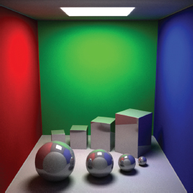
Lighting is at the heart of all CG rendering. Without good lighting, an otherwise beautifully modeled scene will look flat and artificial. Likewise, even the simplest of scenes can be made to look extremely realistic when it is lit accurately. The classic “Cornell box” scene, shown in Figure 11.19, is an excellent example of this.
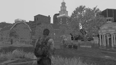
The sequence of screenshots from Naughty Dog’s The Last of Us: Remastered is another good illustration of the importance of lighting. In Figure 11.20, the scene is rendered without textures. Figure 11.21 shows the same scene with diffuse textures applied. The fully lit scene is shown in Figure 11.22. Notice the marked jump in realism when lighting is applied to the scene.
The term shading is often used as a loose generalization of lighting plus other visual effects. As such, “shading” encompasses procedural deformation of vertices to simulate the motion of a water surface, generation of hair curves or fur shells, tessellation of high-order surfaces, and pretty much any other calculation that’s required to render a scene.
In the following sections, we’ll lay the foundations of lighting that we’ll need in order to understand graphics hardware and the rendering pipeline. We’ll return to the topic of lighting in Section 11.3, where we’ll survey some advanced lighting and shading techniques.
11.1.3.1 Local and Global Illumination Models
Rendering engines use various mathematical models of light-surface and light-volume interactions called light transport models. The simplest models only account for direct lighting in which light is emitted, bounces off a single object in the scene, and then proceeds directly to the imaging plane of the virtual camera. Such simple models are called local illumination models, because only the local effects of light on a single object are considered; objects do not affect one another’s appearance in a local lighting model. Not surprisingly, local models were the first to be used in games, and they are still in use today—local lighting can produce surprisingly realistic results in some circumstances.

True photorealism can only be achieved by accounting for indirect lighting, where light bounces multiple times off many surfaces before reaching the virtual camera. Lighting models that account for indirect lighting are called global illumination models. Some global illumination models are targeted at simulating one specific visual phenomenon, such as producing realistic shadows, modeling reflective surfaces, accounting for interreflection between objects (where the color of one object affects the colors of surrounding objects), and modeling caustic effects (the intense reflections from water or a shiny metal surface). Other global illumination models attempt to provide a holistic account of a wide range of optical phenomena. Ray tracing and radiosity methods are examples of such technologies.
Global illumination is described completely by a mathematical formulation known as the rendering equation or shading equation. It was introduced in 1986 by J. T. Kajiya as part of a seminal SIGGRAPH paper. In a sense, every rendering technique can be thought of as a full or partial solution to the rendering equation, although they differ in their fundamental approach to solving it and in the assumptions, simplifications and approximations they make. See http://en.wikipedia.org/wiki/Rendering_equation, [10], [2] and virtually any other text on advanced rendering and lighting for more details on the rendering equation.
11.1.3.2 The Phong Lighting Model
The most common local lighting model employed by game rendering engines is the Phong reflection model. It models the light reflected from a surface as a sum of three distinct terms:
Figure 11.23 shows how the ambient, diffuse and specular terms add together to produce the final intensity and color of a surface.

To calculate Phong reflection at a specific point on a surface, we require a number of input parameters. The Phong model is normally applied to all three color channels (R, G and B) independently, so all of the color parameters in the following discussion are three-element vectors. The inputs to the Phong model are:
In the Phong model, the intensity I of light reflected from a point can be expressed with the following vector equation:
where the sum is taken over all lights i affecting the point in question. Recall that the operator ⊗ represents the component-wise multiplication of two vectors (the so-called Hadamard product). This expression can be broken into three scalar equations, one for each color channel, as follows:

In these equations, the vector Ri = [Rix Riy Riz] is the reflection of the light ray’s direction vector Li about the surface normal N.
The vector Ri can be easily calculated via a bit of vector math (see Figure 11.24). Any vector can be expressed as a sum of its normal and tangential components. For example, we can break up the light direction vector L as follows:
We know that the dot product (N · L) represents the projection of L normal to the surface (a scalar quantity). So the normal component LN is just the unit normal vector N scaled by this dot product:
The reflected vector R has the same normal component as L but the opposite tangential component (−LT). So we can find R as follows:
This equation can be used to find all of the Ri values corresponding to the light directions Li.
Blinn-Phong
The Blinn-Phong lighting model is a variation on Phong shading that calculates specular reflection in a slightly different way. We define the vector H to be the vector that lies halfway between the view vector V and the light direction vector L. The Blinn-Phong specular component is then (N · H)a, as opposed to Phong’s (R · V)α. The exponent a is slightly different than the Phong exponent a, but its value is chosen in order to closely match the equivalent Phong specular term.
The Blinn-Phong model offers increased runtime efficiency at the cost of some accuracy, although it actually matches empirical results more closely than Phong for some kinds of surfaces. The Blinn-Phong model was used almost exclusively in early computer games and was hard-wired into the fixed-function pipelines of early GPUs. See http://en.wikipedia.org/wiki/Blinn%E2%80%93Phong_shading_model for more details.
BRDF Plots
The three terms in the Phong lighting model are special cases of a general local reflection model known as a bidirectional reflection distribution function (BRDF). A BRDF calculates the ratio of the outgoing (reflected) radiance along a given viewing direction V to the incoming irradiance along the incident ray L.
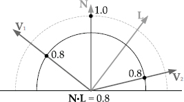
A BRDF can be visualized as a hemispherical plot, where the radial distance from the origin represents the intensity of the light that would be seen if the reflection point were viewed from that direction. The diffuse Phong reflection term is kD (N · L). This term only accounts for the incoming illumination ray L, not the viewing angle V. Hence the value of this term is the same for all viewing angles. If we were to plot this term as a function of the viewing angle in three dimensions, it would look like a hemisphere centered on the point at which we are calculating the Phong reflection. This is shown in two dimensions in Figure 11.25.
The specular term of the Phong model is kD (R · V)α. This term is dependent on both the illumination direction L and the viewing direction V. It produces a specular “hot spot” when the viewing angle aligns closely with the reflection R of the illumination direction L about the surface normal. However, its contribution falls off very quickly as the viewing angle diverges from the reflected illumination direction. This is shown in two dimensions in Figure 11.26.

11.1.3.3 Modeling Light Sources
In addition to modeling the light’s interactions with surfaces, we need to describe the sources of light in the scene. As with all things in real-time rendering, we approximate real-world light sources using various simplified models.
Static Lighting
The fastest lighting calculation is the one you don’t do at all. Lighting is therefore performed offline whenever possible. We can precalculate Phong reflection at the vertices of a mesh and store the results as diffuse vertex color attributes. We can also precalculate lighting on a per-pixel basis and store the results in a kind of texture map known as a light map. At runtime, the light map texture is projected onto the objects in the scene in order to determine the light’s effects on them.
You might wonder why we don’t just bake lighting information directly into the diffuse textures in the scene. There are a few reasons for this. For one thing, diffuse texture maps are often tiled and/or repeated throughout a scene, so baking lighting into them wouldn’t be practical. Instead, a single light map is usually generated per light source and applied to any objects that fall within that light’s area of influence. This approach permits dynamic objects to move past a light source and be properly illuminated by it. It also means that our light maps can be of a different (often lower) resolution than our diffuse texture maps. Finally, a “pure” light map usually compresses better than one that includes diffuse color information.


Ambient Lights
An ambient light corresponds to the ambient term in the Phong lighting model. This term is independent of the viewing angle and has no specific direction. An ambient light is therefore represented by a single color, corresponding to the A color term in the Phong equation (which is scaled by the surface’s ambient reflectivity kA at runtime). The intensity and color of ambient light may vary from region to region within the game world.
Directional Lights
A directional light models a light source that is effectively an infinite distance away from the surface being illuminated—like the sun. The rays emanating from a directional light are parallel, and the light itself does not have any particular location in the game world. A directional light is therefore modeled as a light color C and a direction vector L. A directional light is depicted in Figure 11.27.
Point (Omnidirectional) Lights
A point light (omnidirectional light) has a distinct position in the game world and radiates uniformly in all directions. The intensity of the light is usually considered to fall off with the square of the distance from the light source, and beyond a predefined maximum radius its effects are simply clamped to zero. A point light is modeled as a light position P, a source color/intensity C and a maximum radius rmax. The rendering engine only applies the effects of a point light to those surfaces that fall within its sphere of influence (a significant optimization). Figure 11.28 illustrates a point light.
Spot Lights
A spot light acts like a point light whose rays are restricted to a cone-shaped region, like a flashlight. Usually two cones are specified with an inner and an outer angle. Within the inner cone, the light is considered to be at full intensity. The light intensity falls off as the angle increases from the inner to the outer angle, and beyond the outer cone it is considered to be zero. Within both cones, the light intensity also falls off with radial distance. A spot light is modeled as a position P, a source color C, a central direction vector L, a maximum radius rmax and inner and outer cone angles θmin and θmax. Figure 11.29 illustrates a spot light source.

Area Lights
All of the light sources we’ve discussed thus far radiate from an idealized point, either at infinity or locally. A real light source almost always has a nonzero area—this is what gives rise to the umbra and penumbra in the shadows it casts.
Rather than trying to model area lights explicitly, CG engineers often use various “tricks” to account for their behavior. For example to simulate a penumbra, we might cast multiple shadows and blend the results, or we might blur the edges of a sharp shadow in some manner.
Emissive Objects
Some surfaces in a scene are themselves light sources. Examples include flashlights, glowing crystal balls, flames from a rocket engine and so on. Glowing surfaces can be modeled using an emissive texture map—a texture whose colors are always at full intensity, independent of the surrounding lighting environment. Such a texture could be used to define a neon sign, a car’s headlights and so on.
Some kinds of emissive objects are rendered by combining multiple techniques. For example, a flashlight might be rendered using an emissive texture for when you’re looking head-on into the beam, a colocated spot light that casts light into the scene, a yellow translucent mesh to simulate the light cone, some camera-facing transparent cards to simulate lens flare (or a bloom effect if high dynamic range lighting is supported by the engine), and a projected texture to produce the caustic effect that a flashlight has on the surfaces it illuminates. The flashlight in Luigi’s Mansion is a great example of this kind of effect combination, as shown in Figure 11.30.
11.1.4 The Virtual Camera
In computer graphics, the virtual camera is much simpler than a real camera or the human eye. We treat the camera as an ideal focal point with a rectangular virtual sensing surface called the imaging rectangle floating some small distance in front of it. The imaging rectangle consists of a grid of square or rectangular virtual light sensors, each corresponding to a single pixel on-screen. Rendering can be thought of as the process of determining what color and intensity of light would be recorded by each of these virtual sensors.

11.1.4.1 View Space
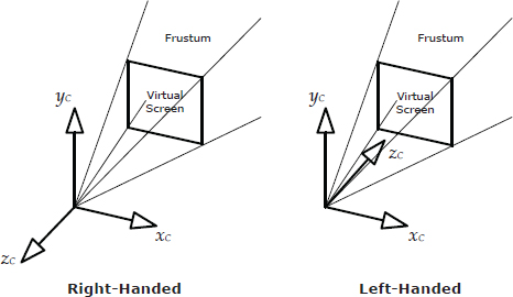
The focal point of the virtual camera is the origin of a 3D coordinate system known as view space or camera space. The camera usually “looks” down the positive or negative z-axis in view space, with y up and x to the left or right. Typical left- and right-handed view-space axes are illustrated in Figure 11.31.
The camera’s position and orientation can be specified using a view-to-world matrix, just as a mesh instance is located in the scene with its model-to-world matrix. If we know the position vector and three unit basis vectors of camera space, expressed in world-space coordinates, the view-to-world matrix can be written as follows, in a manner analogous to that used to construct a model-to-world matrix:

When rendering a triangle mesh, its vertices are transformed first from model space to world space, and then from world space to view space. To perform this latter transformation, we need the world-to-view matrix, which is the inverse of the view-to-world matrix. This matrix is sometimes called the view matrix:
Be careful here. The fact that the camera’s matrix is inverted relative to the matrices of the objects in the scene is a common point of confusion and bugs among new game developers.
The world-to-view matrix is often concatenated to the model-to-world matrix prior to rendering a particular mesh instance. This combined matrix is called the model-view matrix in OpenGL. We precalculate this matrix so that the rendering engine only needs to do a single matrix multiply when transforming vertices from model space into view space:
11.1.4.2 Projections
In order to render a 3D scene onto a 2D image plane, we use a special kind of transformation known as a projection. The perspective projection is the most common projection in computer graphics, because it mimics the kinds of images produced by a typical camera. With this projection, objects appear smaller the farther away they are from the camera—an effect known as perspective foreshortening.
The length-preserving orthographic projection is also used by some games, primarily for rendering plan views (e.g., front, side and top) of 3D models or game levels for editing purposes, and for overlaying 2D graphics onto the screen for heads-up displays and the like. Figure 11.32 illustrates how a cube would look when rendered with these two types of projections.

11.1.4.3 The View Volume and the Frustum
The region of space that the camera can “see” is known as the view volume. A view volume is defined by six planes. The near plane corresponds to the virtual image-sensing surface. The four side planes correspond to the edges of the virtual screen. The far plane is used as a rendering optimization to ensure that extremely distant objects are not drawn. It also provides an upper limit for the depths that will be stored in the depth buffer (see Section 11.1.4.8).
When rendering the scene with a perspective projection, the shape of the view volume is a truncated pyramid known as a frustum. When using an orthographic projection, the view volume is a rectangular prism. Perspective and orthographic view volumes are illustrated in Figure 11.33 and Figure 11.34, respectively.
The six planes of the view volume can be represented compactly using six four-element vectors (nix, niy, niz, di), where n = (nx, ny, nz) is the plane normal and d is its perpendicular distance from the origin. If we prefer the point-normal plane representation, we can also describe the planes with six pairs of vectors (Qi, ni), where Q is the arbitrary point on the plane and n is the plane normal. (In both cases, i is an index representing the six planes.)


11.1.4.4 Projection and Homogeneous Clip Space
Both perspective and orthographic projections transform points in view space into a coordinate space called homogeneous clip space. This three-dimensional space is really just a warped version of view space. The purpose of clip space is to convert the camera-space view volume into a canonical view volume that is independent both of the kind of projection used to convert the 3D scene into 2D screen space, and of the resolution and aspect ratio of the screen onto which the scene is going to be rendered.
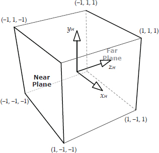
In clip space, the canonical view volume is a rectangular prism extending from −1 to +1 along the x- and y-axes. Along the z-axis, the view volume extends either from −1 to +1 (OpenGL) or from 0 to 1 (DirectX). We call this coordinate system “clip space” because the view volume planes are axis-aligned, making it convenient to clip triangles to the view volume in this space (even when a perspective projection is being used). The canonical clip-space view volume for OpenGL is depicted in Figure 11.35. Notice that the z-axis of clip space goes into the screen, with y up and x to the right. In other words, homogeneous clip space is usually left-handed. A left-handed convention is used here because it causes increasing z values to correspond to increasing depth into the screen, with y increasing up and x increasing to the right as usual.
Perspective Projection
An excellent explanation of perspective projection is given in Section 4.5.1 of [32], so we won’t repeat it here. Instead, we’ll simply present the perspective projection matrix MV→H below. (The subscript V → H indicates that this matrix transforms vertices from view space into homogeneous clip space.) If we take view space to be right-handed, then the near plane intersects the z-axis at z = −n, and the far plane intersects it at z = −f. The virtual screen’s left, right, bottom, and top edges lie at x = l, x = r, y = b and y = t on the near plane, respectively. (Typically the virtual screen is centered on the cameraspace z-axis, in which case l = −r and b = −t, but this isn’t always the case.) Using these definitions, the perspective projection matrix for OpenGL is as follows:
DirectX defines the z-axis extents of the clip-space view volume to lie in the range [0, 1] rather than in the range [−1, 1] as OpenGL does. We can easily adjust the perspective projection matrix to account for DirectX’s conventions as follows:
Division by z
Perspective projection results in each vertex’s x- and y-coordinates being divided by its z-coordinate. This is what produces perspective foreshortening. To understand why this happens, consider multiplying a view-space point pV expressed in four-element homogeneous coordinates by the OpenGL perspective projection matrix:
The result of this multiplication takes the form
When we convert any homogeneous vector into three-dimensional coordinates, the x-, y- and z-components are divided by the w-component:
So, after dividing Equation (11.1) by the homogeneous w-component, which is really just the negative view-space z-coordinate −pVz, we have:
Thus, the homogeneous clip-space coordinates have been divided by the viewspace z-coordinate, which is what causes perspective foreshortening.
Perspective-Correct Vertex Attribute Interpolation
In Section 11.1.2.4, we learned that vertex attributes are interpolated in order to determine appropriate values for them within the interior of a triangle. Attribute interpolation is performed in screen space. We iterate over each pixel of the screen and attempt to determine the value of each attribute at the corresponding location on the surface of the triangle. When rendering a scene with a perspective projection, we must do this very carefully so as to account for perspective foreshortening. This is known as perspective-correct attribute interpolation.
A derivation of perspective-correct interpolation is beyond our scope, but suffice it to say that we must divide our interpolated attribute values by the corresponding z-coordinates (depths) at each vertex. For any pair of vertex attributes A1 and A2, we can write the interpolated attribute at a percentage t of the distance between them as follows:
Refer to [32] for an excellent derivation of the math behind perspective-correct attribute interpolation.
Orthographic Projection
An orthographic projection is performed by the following matrix:
This is just an everyday scale-and-translate matrix. (The upper-left 3 × 3 contains a diagonal nonuniform scaling matrix, and the lower row contains the translation.) Since the view volume is a rectangular prism in both view space and clip space, we need only scale and translate our vertices to convert from one space to the other.

11.1.4.5 Screen Space and Aspect Ratios
Screen space is a two-dimensional coordinate system whose axes are measured in terms of screen pixels. The x-axis typically points to the right, with the origin at the top-left corner of the screen and y pointing down. (The reason for the inverted y-axis is that CRT monitors scan the screen from top to bottom.) The ratio of screen width to screen height is known as the aspect ratio. The most common aspect ratios are 4:3 (the aspect ratio of a traditional television screen) and 16:9 (the aspect ratio of a movie screen or HDTV). These aspect ratios are illustrated in Figure 11.36.
We can render triangles expressed in homogeneous clip space by simply drawing their (x, y) coordinates and ignoring z. But before we do, we scale and shift the clip-space coordinates so that they lie in screen space rather than within the normalized unit square. This scale-and-shift operation is known as screen mapping.
11.1.4.6 The Frame Buffer
The final rendered image is stored in a bitmapped color buffer known as the frame buffer. Pixel colors are usually stored in RGBA8888 format, although other frame buffer formats are supported by most graphics cards as well. Some common formats include RGB565, RGB5551, and one or more paletted modes.
The display hardware (CRT, flat-screen monitor, HDTV, etc.) reads the contents of the frame buffer at a periodic rate of 60 Hz for NTSC televisions used in North America and Japan, or 50 Hz for PAL/SECAM televisions used in Europe and many other places in the world. Rendering engines typically maintain at least two frame buffers. While one is being scanned by the display hardware, the other one can be updated by the rendering engine. This is known as double buffering. By swapping or “flipping” the two buffers during the vertical blanking interval (the period during which the CRT’s electron gun is being reset to the top-left corner of the screen), double buffering ensures that the display hardware always scans the complete frame buffer. This avoids a jarring effect known as tearing, in which the upper portion of the screen displays the newly rendered image while the bottom shows the remnants of the previous frame’s image.
Some engines make use of three frame buffers—a technique aptly known as triple buffering. This is done so that the rendering engine can start work on the next frame, even while the previous frame is still being scanned by the display hardware. For example, the hardware might still be scanning buffer A when the engine finishes drawing buffer B. With triple buffering, it can proceed to render a new frame into buffer C, rather than idling while it waits for the display hardware to finish scanning buffer A.
Render Targets
Any buffer into which the rendering engine draws graphics is known as a render target. As we’ll see later in this chapter, rendering engines make use of all sorts of other off-screen render targets in addition to the frame buffers. These include the depth buffer, the stencil buffer and various other buffers used for storing intermediate rendering results.
11.1.4.7 Triangle Rasterization and Fragments
To produce an image of a triangle on-screen, we need to fill in the pixels it overlaps. This process is known as rasterization. During rasterization, the triangle’s surface is broken into pieces called fragments, each one representing a small region of the triangle’s surface that corresponds to a single pixel on the screen. (In the case of multisample antialiasing, a fragment corresponds to a portion of a pixel—see below.)
A fragment is like a pixel in training. Before it is written into the frame buffer, it must pass a number of tests (described in more depth below). If it fails any of these tests, it will be discarded. Fragments that pass the tests are shaded (i.e., their colors are determined), and the fragment color is either written into the frame buffer or blended with the pixel color that’s already there. Figure 11.37 illustrates how a fragment becomes a pixel.
11.1.4.8 Occlusion and the Depth Buffer
When rendering two triangles that overlap each other in screen space, we need some way of ensuring that the triangle that is closer to the camera will appear on top. We could accomplish this by always rendering our triangles in back-to-front order (the so-called painter’s algorithm). However, as shown in Figure 11.38, this doesn’t work if the triangles are intersecting one another.

To implement triangle occlusion properly, independent of the order in which the triangles are rendered, rendering engines use a technique known as depth buffering or z-buffering. The depth buffer is a full-screen buffer that typically contains 24-bit integer or (more rarely) floating-point depth information for each pixel in the frame buffer. (The depth buffer is usually stored in a 32-bits-per-pixel format, with a 24-bit depth value and an 8-bit stencil value packed into each pixel’s 32-bit quadword.) Every fragment has a z-coordinate that measures its depth “into” the screen. (The depth of a fragment is found by interpolating the depths of the triangle’s vertices.) When a fragment’s color is written into the frame buffer, its depth is stored into the corresponding pixel of the depth buffer. When another fragment (from another triangle) is drawn into the same pixel, the engine compares the new fragment’s depth to the depth already present in the depth buffer. If the fragment is closer to the camera (i.e., if it has a smaller depth), it overwrites the pixel in the frame buffer. Otherwise the fragment is discarded.

z-Fighting and the w-Buffer
When rendering parallel surfaces that are very close to one another, it’s important that the rendering engine can distinguish between the depths of the two planes. If our depth buffer had infinite precision, this would never be a problem. Unfortunately, a real depth buffer only has limited precision, so the depth values of two planes can collapse into a single discrete value when the planes are close enough together. When this happens, the more-distant plane’s pixels start to “poke through” the nearer plane, resulting in a noisy effect known as z-fighting.
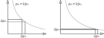
To reduce z-fighting to a minimum across the entire scene, we would like to have equal precision whether we’re rendering surfaces that are close to the camera or far away. However, with z-buffering this is not the case. The precision of clip-space z-depths are not evenly distributed across the entire range from the near plane to the far plane, because of the division by the view-space z-coordinate. Because of the shape of the 1/z curve, most of the depth buffer’s precision is concentrated near the camera.
The plot of the function shown in Figure 11.39 demonstrates this effect. Near the camera, the distance between two planes in view space gets transformed into a reasonably large delta in clip space . But far from the camera, this same separation gets transformed into a tiny delta in clip space. The result is z-fighting, and it becomes rapidly more prevalent as objects get farther away from the camera.
To circumvent this problem, we would like to store view-space z-coordinates in the depth buffer instead of clip-space z-coordinates . View-space z-coordinates vary linearly with the distance from the camera, so using them as our depth measure achieves uniform precision across the entire depth range. This technique is called w-buffering, because the view-space z-coordinate conveniently appears in the w-component of our homogeneous clip-space coordinates. (Recall from Equation (11.1) that .)
The terminology can be very confusing here. The z- and w-buffers store coordinates that are expressed in clip space. But in terms of view-space coordinates, the z-buffer stores 1/z (i.e., ) while the w-buffer stores z (i.e., )!
We should note here that the w-buffering approach is a bit more expensive than its z-based counterpart. This is because with w-buffering, we cannot linearly interpolate depths directly. Depths must be inverted prior to interpolation and then re-inverted prior to being stored in the w-buffer.
11.2 The Rendering Pipeline
Now that we’ve completed our whirlwind tour of the major theoretical and practical underpinnings of triangle rasterization, let’s turn our attention to how it is typically implemented. In real-time game rendering engines, the high-level rendering steps described in Section 11.1 are implemented using a software/hardware architecture known as a pipeline. A pipeline is just an ordered chain of computational stages, each with a specific purpose, operating on a stream of input data items and producing a stream of output data.
Each stage of a pipeline can typically operate independently of the other stages. Hence, one of the biggest advantages of a pipelined architecture is that it lends itself extremely well to parallelization. While the first stage is chewing on one data element, the second stage can be processing the results previously produced by the first stage, and so on down the chain.
Parallelization can also be achieved within an individual stage of the pipeline. For example, if the computing hardware for a particular stage is duplicated N times on the die, N data elements can be processed in parallel by that stage. A parallelized pipeline is shown in Figure 11.40. Ideally the stages operate in parallel (most of the time), and certain stages are capable of operating on multiple data items simultaneously as well.
The throughput of a pipeline measures how many data items are processed per second overall. The pipeline’s latency measures the amount of time it takes for a single data element to make it through the entire pipeline. The latency of an individual stage measures how long that stage takes to process a single item. The slowest stage of a pipeline dictates the throughput of the entire pipeline. It also has an impact on the average latency of the pipeline as a whole. Therefore, when designing a rendering pipeline, we attempt to minimize and balance latency across the entire pipeline and eliminate bottlenecks. In a well-designed pipeline, all the stages operate simultaneously, and no stage is ever idle for very long waiting for another stage to become free.

11.2.1 Overview of the Rendering Pipeline
Some graphics texts divide the rendering pipeline into three coarse-grained stages. In this book, we’ll extend this pipeline back even further, to encompass the offline tools used to create the scenes that are ultimately rendered by the game engine. The high-level stages in our pipeline are:

11.2.1.1 How the Rendering Pipeline Transforms Data
It’s interesting to note how the format of geometry data changes as it passes through the rendering pipeline. The tools and asset conditioning stages deal with meshes and materials. The application stage deals in terms of mesh instances and submeshes, each of which is associated with a single material. During the geometry stage, each submesh is broken down into individual vertices, which are processed largely in parallel. At the conclusion of this stage, the triangles are reconstructed from the fully transformed and shaded vertices. In the rasterization stage, each triangle is broken into fragments, and these fragments are either discarded, or they are eventually written into the frame buffer as colors. This process is illustrated in Figure 11.41.
11.2.1.2 Implementation of the Pipeline
The first two stages of the rendering pipeline are implemented offline, usually executed by a Windows or Linux machine. The application stage is typically run on one or more CPU cores, whereas the geometry and rasterization stages are usually executed by the graphics processing unit (GPU). In the following sections, we’ll explore some of the details of how each of these stages is implemented.
11.2.2 The Tools Stage
In the tools stage, meshes are authored by 3D modelers in a digital content creation (DCC) application like Maya, 3ds Max, Lightwave, Softimage/XSI, SketchUp, etc. The models may be defined using any convenient surface description—NURBS, quads, triangles, etc. However, they are invariably tessellated into triangles prior to rendering by the runtime portion of the pipeline.
The vertices of a mesh may also be skinned. This involves associating each vertex with one or more joints in an articulated skeletal structure, along with weights describing each joint’s relative influence over the vertex. Skinning information and the skeleton are used by the animation system to drive the movements of a model—see Chapter 12 for more details.
Materials are also defined by the artists during the tools stage. This involves selecting a shader for each material, selecting textures as required by the shader, and specifying the configuration parameters and options of each shader. Textures are mapped onto the surfaces, and other vertex attributes are also defined, often by “painting” them with some kind of intuitive tool within the DCC application.
Materials are usually authored using a commercial or custom in-house material editor. The material editor is sometimes integrated directly into the DCC application as a plug-in, or it may be a stand-alone program. Some material editors are live-linked to the game, so that material authors can see what the materials will look like in the real game. Other editors provide an offline 3D visualization view. Some editors even allow shader programs to be written and debugged by the artist or a shader engineer. Such tools allow rapid prototyping of visual effects by connecting various kinds of nodes together with a mouse. These tools generally provide a WYSIWYG display of the resulting material. NVIDIA’s Fx Composer is an example of such a tool. Sadly, NVIDIA is no longer updating Fx Composer, and it only supports shader models up to DirectX 10. But they do offer a new Visual Studio plugin called NVIDIA® Nsight™ Visual Studio Edition. Depicted in Figure 11.42, Nsight provides powerful shader authoring and debugging facilities. The Unreal Engine also provides a graphical shader editor called Material Editor; it is shown in Figure 11.43.
Materials may be stored and managed with the individual meshes. However, this can lead to duplication of data—and effort. In many games, a relatively small number of materials can be used to define a wide range of objects in the game. For example, we might define some standard, reusable materials like wood, rock, metal, plastic, cloth, skin and so on. There’s no reason to duplicate these materials inside every mesh. Instead, many game teams build up a library of materials from which to choose, and the individual meshes refer to the materials in a loosely coupled manner.

11.2.3 The Asset Conditioning Stage
The asset conditioning stage is itself a pipeline, sometimes called the asset conditioning pipeline (ACP) or the tools pipeline. As we saw in Section 7.2.1.4, its job is to export, process and link together multiple types of assets into a cohesive whole. For example, a 3D model is comprised of geometry (vertex and index buffers), materials, textures and an optional skeleton. The ACP ensures that all of the individual assets referenced by a 3D model are available and ready to be loaded by the engine.
Geometric and material data is extracted from the DCC application and is usually stored in a platform-independent intermediate format. The data is then further processed into one or more platform-specific formats, depending on how many target platforms the engine supports. Ideally the platform-specific assets produced by this stage are ready to load into memory and use with little or no postprocessing at runtime. For example, mesh data targeted for the Xbox One or PS4 might be output as index and vertex buffers that are ready to be consumed by the GPU; on the PS3, geometry might be produced in compressed data streams that are ready to be DMA’d to the SPUs for decompression. The ACP often takes the needs of the material/shader into account when building assets. For example, a particular shader might require tangent and bitangent vectors as well as a vertex normal; the ACP could generate these vectors automatically.

High-level scene graph data structures may also be computed during the asset conditioning stage. For example, static-level geometry may be processed in order to build a BSP tree. (As we’ll investigate in Section 11.2.7.4, scene graph data structures help the rendering engine to very quickly determine which objects should be rendered, given a particular camera position and orientation.)
Expensive lighting calculations are often done offline as part of the asset conditioning stage. This is called static lighting; it may include calculation of light colors at the vertices of a mesh (this is called “baked” vertex lighting), construction of texture maps that encode per-pixel lighting information known as light maps, calculation of precomputed radiance transfer (PRT) coefficients (usually represented by spherical harmonic functions) and so on.
11.2.4 The GPU Pipeline
Graphics hardware has evolved around a specialized type of microprocessor known as a graphics processing unit or GPU. As we discussed in Section 4.11, a GPU is designed to maximize throughput of the graphics pipeline, which it achieves through massive parallelization of tasks like vertex processing and per-pixel shading calculations. For example, a modern GPU like the AMD Radeon™ 7970 can achieve a peak performance of 4 TFLOPS, which it does by executing workloads in parallel across 32 compute units, each of which contains four 16-lane SIMD VPUs, which in turn execute pipelined wavefronts consisting of 64 threads each. A GPU can be used to render graphics, but today’s GPUs are also fully programmable, allowing programmers to leverage the awesome computing power of a GPU to execute compute shaders. This is known as general-purpose GPU computing (GPGPU).

Virtually all GPUs break the graphics pipeline into the substages described below and depicted in Figure 11.44. Each stage is shaded to indicate whether its functionality is programmable, fixed but configurable, or fixed and non-configurable.
11.2.4.1 Vertex Shader
This stage is fully programmable. It is responsible for transformation and shading/lighting of individual vertices. The input to this stage is a single vertex (although in practice many vertices are processed in parallel). Its position and normal are typically expressed in model space or world space. The vertex shader handles transformation from model space to view space via the modelview transform. Perspective projection is also applied, as well as per-vertex lighting and texturing calculations, and skinning for animated characters. The vertex shader can also perform procedural animation by modifying the position of the vertex. Examples of this include foliage that sways in the breeze or an undulating water surface. The output of this stage is a fully transformed and lit vertex, whose position and normal are expressed in homogeneous clip space (see Section 11.1.4.4).
On modern GPUs, the vertex shader has full access to texture data—a capability that used to be available only to the pixel shader. This is particularly useful when textures are used as stand-alone data structures like heightmaps or look-up tables.
11.2.4.2 Geometry Shader
This optional stage is also fully programmable. The geometry shader operates on entire primitives (triangles, lines and points) in homogeneous clip space. It is capable of culling or modifying input primitives, and it can also generate new primitives. Typical uses include shadow volume extrusion (see Section 11.3.3.1), rendering the six faces of a cube map (see Section 11.3.1.4), fur fin extrusion around silhouette edges of meshes, creation of particle quads from point data (see Section 11.4.1), dynamic tessellation, fractal subdivision of line segments for lightning effects, cloth simulations, and the list goes on.
11.2.4.3 Stream Output
Some GPUs permit the data that has been processed up to this point in the pipeline to be written back to memory. From there, it can then be looped back to the top of the pipeline for further processing. This feature is called stream output.
Stream output permits a number of intriguing visual effects to be achieved without the aid of the CPU. An excellent example is hair rendering. Hair is often represented as a collection of cubic spline curves. It used to be that hair physics simulation would be done on the CPU. The CPU would also tessellate the splines into line segments. Finally the GPU would render the segments.
With stream output, the GPU can do the physics simulation on the control points of the hair splines within the vertex shader. The geometry shader tessellates the splines, and the stream output feature is used to write the tessellated vertex data to memory. The line segments are then piped back into the top of the pipeline so they can be rendered.
11.2.4.4 Clipping
The clipping stage chops off those portions of the triangles that straddle the frustum. Clipping is done by identifying vertices that lie outside the frustum and then finding the intersection of the triangle’s edges with the planes of the frustum. These intersection points become new vertices that define one or more clipped triangles.
This stage is fixed in function, but it is somewhat configurable. For example, user-defined clipping planes can be added in addition to the frustum planes. This stage can also be configured to cull triangles that lie entirely outside the frustum.
11.2.4.5 Screen Mapping
Screen mapping simply scales and shifts the vertices from homogeneous clip space into screen space. This stage is entirely fixed and non-configurable.
11.2.4.6 Triangle Set-up
During triangle set-up, the rasterization hardware is initialized for efficient conversion of the triangle into fragments. This stage is not configurable.
11.2.4.7 Triangle Traversal
Each triangle is broken into fragments (i.e., rasterized) by the triangle traversal stage. Usually one fragment is generated for each pixel, although with certain antialiasing techniques, multiple fragments may be created per pixel (see Section 11.1.4.7). The triangle traversal stage also interpolates vertex attributes in order to generate per-fragment attributes for processing by the pixel shader. Perspective-correct interpolation is used where appropriate. This stage’s functionality is fixed and not configurable.
11.2.4.8 Early z-Test
Many graphics cards are capable of checking the depth of the fragment at this point in the pipeline, discarding it if it is being occluded by the pixel already in the frame buffer. This allows the (potentially very expensive) pixel shader stage to be skipped entirely for occluded fragments.
Surprisingly, not all graphics hardware supports depth testing at this stage of the pipeline. In older GPU designs, the z-test was done along with alpha testing, after the pixel shader had run. For this reason, this stage is called the early z-test or early depth test stage.
11.2.4.9 Pixel Shader
This stage is fully programmable. Its job is to shade (i.e., light and otherwise process) each fragment. The pixel shader can also discard fragments, for example because they are deemed to be entirely transparent. The pixel shader can address one or more texture maps, run per-pixel lighting calculations, and do whatever else is necessary to determine the fragment’s color.
The input to this stage is a collection of per-fragment attributes (which have been interpolated from the vertex attributes by the triangle traversal stage). The output is a single color vector describing the desired color of the fragment.
11.2.4.10 Merging / Raster Operations Stage
The final stage of the pipeline is known as the merging stage or blending stage, also known as the raster operations stage or ROP in NVIDIA parlance. This stage is not programmable, but it is highly configurable. It is responsible for running various fragment tests including the depth test (see Section 11.1.4.8), alpha test (in which the values of the fragment’s and pixel’s alpha channels can be used to reject certain fragments) and stencil test (see Section 11.3.3.1).
If the fragment passes all of the tests, its color is blended (merged) with the color that is already present in the frame buffer. The way in which blending occurs is controlled by the alpha blending function—a function whose basic structure is hard-wired, but whose operators and parameters can be configured in order to produce a wide variety of blending operations.
Alpha blending is most commonly used to render semitransparent geometry. In this case, the following blending function is used:
The subscripts S and D stand for “source” (the incoming fragment) and “destination” (the pixel in the frame buffer), respectively. Therefore, the color that is written into the frame buffer (C′D) is a weighted average of the existing frame buffer contents (CD) and the color of the fragment being drawn (CS). The blend weight (AS) is just the source alpha of the incoming fragment.
For alpha blending to look right, the semitransparent and translucent surfaces in the scene must be sorted and rendered in back-to-front order, after the opaque geometry has been rendered to the frame buffer. This is because after alpha blending has been performed, the depth of the new fragment overwrites the depth of the pixel with which it was blended. In other words, the depth buffer ignores transparency (unless depth writes have been turned off, of course). If we are rendering a stack of translucent objects on top of an opaque backdrop, the resulting pixel color should ideally be a blend between the opaque surface’s color and the colors of all of the translucent surfaces in the stack. If we try to render the stack in any order other than back-to-front, depth-test failures will cause some of the translucent fragments to be discarded, resulting in an incomplete blend (and a rather odd-looking image).
Other alpha blending functions can be defined as well, for purposes other than transparency blending. The general blending equation takes the form C′D = (wS ⊗ CS) + (wD ⊗ CD), where the weighting factors wS and wD can be selected by the programmer from a predefined set of values including zero, one, source or destination color, source or destination alpha and one minus the source or destination color or alpha. The operator ⊗ is either a regular scalar-vector multiplication or a component-wise vector-vector multiplication (a Hadamard product—see Section 5.2.4.1) depending on the data types of wS and wD.
11.2.5 Programmable Shaders
Now that we have an end-to-end picture of the GPU pipeline in mind, let’s take a deeper look at the most interesting part of the pipeline—the programmable shaders. Shader architectures have evolved significantly since their introduction with DirectX 8. Early shader models supported only low-level assembly language programming, and the instruction set and register set of the pixel shader differed significantly from those of the vertex shader. DirectX 9 brought with it support for high-level C-like shader languages such as Cg (C for graphics), HLSL (High-Level Shading Language—Microsoft’s implementation of the Cg language) and GLSL (OpenGL shading language). With DirectX 10, the geometry shader was introduced, and with it came a unified shader architecture called shader model 4.0 in DirectX parlance. In the unified shader model, all three types of shaders support roughly the same instruction set and have roughly the same set of capabilities, including the ability to read texture memory.
A shader takes a single element of input data and transforms it into zero or more elements of output data.
11.2.5.1 Accessing Memory
Because the GPU implements a data processing pipeline, access to RAM is carefully controlled. A shader program usually cannot read from or write to memory directly. Instead, its memory accesses are limited to two methods: registers and texture maps.
However, we should note that these restrictions are lifted on systems in which the GPU and CPU share memory directly. For example, the AMD Jaguar system on a chip (SoC) that sits at the heart of the PlayStation 4 is an example of a heterogeneous system architecture (HSA). On a non-HSA system, the CPU and GPU are typically separate devices, each with its own private memory, and each usually residing on a separate circuit board. Transferring data between the two processors requires cumbersome, high-latency communication over a specialized bus such as AGP or PCIe. With HSA, the CPU and GPU share a single unified memory store called a heterogeneous unified memory architecture (hUMA). Shaders running on a system with hUMA, like the PS4, can therefore be passed a shader resource table (SRT) as input. This is just a pointer to a C/C++ struct in memory that can be read from or written to by both the CPU and the shader running on the GPU. On the PS4, SRTs take the place of the constant registers described in the following sections.
Shader Registers
A shader can access RAM indirectly via registers. All GPU registers are in 128-bit SIMD format. Each register is capable of holding four 32-bit floating-point or integer values (represented by the float4 data type in the Cg language). Such a register can contain a four-element vector in homogeneous coordinates or a color in RGBA format, with each component in 32-bit floating-point format. Matrices can be represented by groups of three or four registers (represented by built-in matrix types like float4x4 in Cg). A GPU register can also be used to hold a single 32-bit scalar, in which case the value is usually replicated across all four 32-bit fields. Some GPUs can operate on 16-bit fields, known as halfs. (Cg provides various built-in types like half4 and half4x4 for this purpose.)
Registers come in four flavors, as follows:
The application provides the values of the constant registers when it submits primitives for rendering. The GPU automatically copies vertex or fragment attribute data from video RAM into the appropriate input registers prior to calling the shader program, and it also writes the contents of the output registers back into RAM at the conclusion of the program’s execution so that the data can be passed to the next stage of the pipeline.
GPUs typically cache output data so that it can be reused without being recalculated. For example, the post-transform vertex cache stores the most-recently processed vertices emitted by the vertex shader. If a triangle is encountered that refers to a previously processed vertex, it will be read from the posttransform vertex cache if possible—the vertex shader need only be called again if the vertex in question has since been ejected from the cache to make room for newly processed vertices.
Textures
A shader also has direct read-only access to texture maps. Texture data is addressed via texture coordinates, rather than via absolute memory addresses. The GPU’s texture samplers automatically filter the texture data, blending values between adjacent texels or adjacent mipmap levels as appropriate. Texture filtering can be disabled in order to gain direct access to the values of particular texels. This can be useful when a texture map is used as a data table, for example.
Shaders can only write to texture maps in an indirect manner—by rendering the scene to an off-screen frame buffer that is interpreted as a texture map by subsequent rendering passes. This feature is known as render to texture.
11.2.5.2 Introduction to High-Level Shader Language Syntax
High-level shader languages like Cg and GLSL are modeled after the C programming language. The programmer can declare functions, define a simple struct, and perform arithmetic. However, as we said above, a shader program only has access to registers and textures. As such, the struct and variable we declare in Cg or GLSL is mapped directly onto registers by the shader compiler. We define these mappings in the following ways:
struct members can be suffixed with a colon followed by a keyword known as a semantic. The semantic tells the shader compiler to bind the variable or data member to a particular vertex or fragment attribute. For example, in a vertex shader we might declare an input struct whose members map to the position and color attributes of a vertex as follows:
struct VtxOut
{
 float4 pos : POSITION; // map to position attribute
 float4 color : COLOR; // map to color attribute
};
struct should map to input or output registers from the context in which it is used. If a variable is passed as an argument to the shader program’s main function, it is assumed to be an input; if it is the return value of the main function, it is taken to be an output.
 VtxOut vshaderMain(VtxIn in) // maps to input registers
 {
 VtxOut out;
// …
return out; // maps to output registers
}
uniform. For example, the model-view matrix could be passed to a vertex shader as follows:
 VtxOut vshaderMain(
 VtxIn in,
 uniform float4x4 modelViewMatrix)
 {
 VtxOut out;
 // …
 return out;
}
Arithmetic operations can be performed by invoking C-style operators, or by calling intrinsic functions as appropriate. For example, to multiply the input vertex position by the model-view matrix, we could write:
VtxOut vshaderMain(VtxIn in,
 uniform float4x4 modelViewMatrix)
{
 VtxOut out;
 out.pos = mul(modelViewMatrix, in.pos);
 out.color = float4(0, 1, 0, 1); // RGBA green
 return out;
}
Data is obtained from textures by calling special intrinsic functions that read the value of the texels at a specified texture coordinate. A number of variants are available for reading one-, two- and three-dimensional textures in various formats, with and without filtering. Special texture addressing modes are also available for accessing cube maps and shadow maps. References to the texture maps themselves are declared using a special data type known as a texture sampler declaration. For example, the data type sampler2D represents a reference to a typical two-dimensional texture. The following simple Cg pixel shader applies a diffuse texture to a triangle:
struct FragmentOut
{
 float4 color : COLOR;
};
FragmentOut pshaderMain(float2 uv : TEXCOORD0,
  uniform sampler2D texture)
{
 FragmentOut out;
 // look up texel at (u,v)
 out.color = tex2D(texture, uv);
 return out;
}
11.2.5.3 Effect Files
By itself, a shader program isn’t particularly useful. Additional information is required by the GPU pipeline in order to call the shader program with meaningful inputs. For example, we need to specify how the application-specified parameters, like the model-view matrix, light parameters and so on, map to the uniform variables declared in the shader program. In addition, some visual effects require two or more rendering passes, but a shader program only describes the operations to be applied during a single rendering pass. If we are writing a game for the PC platform, we will need to define “fallback” versions of some of our more-advanced rendering effects, so that they will work even on older graphics cards. To tie our shader program(s) together into a complete visual effect, we turn to a file format known as an effect file.
Different rendering engines implement effects in slightly different ways. In Cg, the effect file format is known as CgFX. OGRE uses a file format very similar to CgFX known as a material file. GLSL effects can be described using the COLLADA format, which is based on XML. Despite the differences, effects generally take on the following hierarchical format:
11.2.5.4 Further Reading
In this section, we’ve only had a small taste of what high-level shader programming is like—a complete tutorial is beyond our scope here. For a much more detailed introduction to Cg shader programming, refer to the Cg tutorial available on NVIDIA’s website at https://developer.nvidia.com/content/hello-cg-introductory-tutorial.
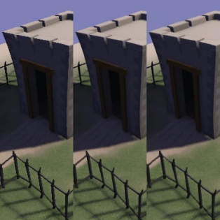
11.2.6 Antialiasing
When a triangle is rasterized, its edges can look jagged—the familiar “stair step” effect we have all come to know and love (or hate). Technically speaking, aliasing arises because we are using a discrete set of pixels to sample an image that is really a smooth, continuous two-dimensional signal. (See Section 14.3.2.1 for a detailed discussion of sampling and aliasing.)
The term antialiasing describes any technique that reduces the visual artifacts caused by aliasing. There are many different ways to antialias a rendered scene. The net effect of pretty much all of them is to “soften” the edges of rendered triangles by blending them with surrounding pixels. Each technique has unique performance, memory-usage and quality characteristics. Figure 11.45 shows a scene rendered first without antialiasing, then with 4× MSAA and finally with Nvidia’s FXAA technique.
11.2.6.1 Full-Screen Antialiasing (FSAA)
In this technique, also known as super-sampled antialiasing (SSAA), the scene is rendered into a frame buffer that is larger than the actual screen. Once rendering of the frame is complete, the resulting oversized image is downsampled to the desired resolution. In 4× supersampling, the rendered image is twice as wide and twice as tall as the screen, resulting in a frame buffer that occupies four times the memory. It also requires four times the GPU processing power because the pixel shader must be run four times for each screen pixel. As you can see, FSAA is an incredibly expensive technique both in terms of memory consumption and GPU cycles. As such, it is rarely used in practice.
11.2.6.2 Multisampled Antialiasing (MSAA)
Multisampled antialiasing is a technique that provides visual quality comparable to that of FSAA, while consuming a great deal less GPU bandwidth (and the same amount of video RAM). The MSAA approach is based on the observation that, thanks to the natural antialiasing effect of texture mipmapping, aliasing tends to be a problem primarily at the edges of triangles, not in their interiors.
To understand how MSAA works, recall that the process of rasterizing a triangle really boils down to three distinct operations: (1) Determining which pixels the triangle overlaps (coverage), (2) determining whether or not each pixel is occluded by some other triangle (depth testing) and (3) determining the color of each pixel, presuming that the coverage and depth tests tell us that the pixel should in fact be drawn (pixel shading).
When rasterizing a triangle without antialiasing, the coverage test, depth test and pixel shading operations are all run at a single idealized point within each screen pixel, usually located at its center. In MSAA, the coverage and depth tests are run for N points known as subsamples within each screen pixel. N is typically chosen to be 2, 4, 5, 8 or 16. However, the pixel shader is only run once per screen pixel, no matter how many subsamples we use. This gives MSAA a big advantage over FSAA in terms of GPU bandwidth, because shading is typically a great deal more expensive than coverage and depth testing.
In N× MSAA, the depth, stencil and color buffers are each allocated to be N times as large as they would otherwise be. For each screen pixel, these buffers contain N “slots,” one slot for each subsample. When rasterizing a triangle, the coverage and depth tests are run N times for the N subsamples within each fragment of the triangle. If at least one of the N tests indicates that the fragment should be drawn, the pixel shader is run once. The color obtained from the pixel shader is then stored only into those slots that correspond to the subsamples that fell inside the triangle. Once the entire scene has been rendered, the oversized color buffer is downsampled to yield the final screen-resolution image. This process involves averaging the color values found in the N subsample slots for each screen pixel. The net result is an antialiased image with a shading cost equal to that of a non-antialiased image.
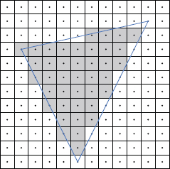
In Figure 11.46 we see a triangle that has been rasterized without antialiasing. Figure 11.47 illustrates the 4× MSAA technique. For more information on MSAA, see http://mynameismjp.wordpress.com/2012/10/24/msaa-overview.
11.2.6.3 Coverage Sample Antialiasing (CSAA)
This technique is an optimization of the MSAA technique pioneered by Nvidia. For 4× CSAA, the pixel shader is run once, the depth test and color storage is done for four subsample points per fragment, but the pixel coverage test is performed for 16 “coverage subsamples” per fragment. This produces finer-grained color blending at the edges of triangles, similar to what you’d see with 8 × or 16 × MSAA, but at the memory and GPU cost of 4 × MSAA.
11.2.6.4 Morphological Antialiasing (MLAA)
Morphological antialiasing focuses its efforts on correcting only those regions of a scene that suffer the most from the effects of aliasing. In MLAA, the scene is rendered at normal size, and then scanned in order to identify stair-stepped patterns. When these patterns are found, they are blurred to reduce the effects of aliasing. Fast approximate antialiasing (FXAA) is an optimized technique developed by Nvidia that is similar to MLAA in its approach.

For a detailed discussion of MLAA, see https://intel.ly/2HhrQWX. FXAA is described in detail here: https://bit.ly/1mIzCTv.
11.2.6.5 Subpixel Morphological Antialiasing (SMAA)
Subpixel Morphological Antialiasing (SMAA) combines morphological antialiasing (MLAA and FXAA) techniques with multisampling/supersampling strategies (MSAA, SSAA) to produce more accurate subpixel features. Like FXAA, it’s an inexpensive technique, but it blurs the final image less than FXAA. For these reasons, it’s arguably the best AA solution available today. A detailed coverage of this topic is beyond our scope in this book, but you can read more about SMAA at http://www.iryoku.com/smaa/.
11.2.7 The Application Stage
Now that we understand how the GPU works, we can discuss the pipeline stage that is responsible for driving it—the application stage. This stage has three roles:
DrawIndexedPrimitive() (DirectX) or glDrawArrays() (OpenGL), or via direct construction of the GPU command list. The geometry may be sorted for optimal rendering performance. Geometry might be submitted more than once if the scene needs to be rendered in multiple passes.In the following sections, we’ll briefly explore how the application stage performs these tasks.
11.2.7.1 Visibility Determination
The cheapest triangles are the ones you never draw. So it’s incredibly important to cull objects from the scene that do not contribute to the final rendered image prior to submitting them to the GPU. The process of constructing the list of visible mesh instances is known as visibility determination.
Frustum Culling
In frustum culling, all objects that lie entirely outside the frustum are excluded from our render list. Given a candidate mesh instance, we can determine whether or not it lies inside the frustum by performing some simple tests between the object’s bounding volume and the six frustum planes. The bounding volume is usually a sphere, because spheres are particularly easy to cull. For each frustum plane, we move the plane outward a distance equal to the radius of the sphere, then we determine on which side of each modified plane the center point of the sphere lies. If the sphere is found to be on the front side of all six modified planes, the sphere is inside the frustum.
In practice, we don’t need to actually move the frustum planes. Recall from Equation (5.13) that the perpendicular distance h from a point to a plane can be calculated by plugging the point directly into the plane equation as follows: h = ax + by + cz + d = n · P − n · P0 (see Section 5.6.3). So all we need to do is plug the center point of our bounding sphere into the plane equations for each frustum plane, giving us a value of hi for each plane i, and then we can compare the hi values to the radius of the bounding sphere to determine whether or not it lies inside each plane.
A scene graph data structure, described in Section 11.2.7.4, can help optimize frustum culling by allowing us to ignore objects whose bounding spheres are nowhere close to being inside the frustum.
Occlusion and Potentially Visible Sets
Even when objects lie entirely within the frustum, they may occlude one another. Removing objects from the visible list that are entirely occluded by other objects is called occlusion culling. In crowded environments viewed from ground level, there can be a great deal of inter-object occlusion, making occlusion culling extremely important. In less crowded scenes, or when scenes are viewed from above, much less occlusion may be present, and the cost of occlusion culling may outweigh its benefits.
Gross occlusion culling of a large-scale environment can be done by pre-calculating a potentially visible set (PVS). For any given camera vantage point, a PVS lists those scene objects that might be visible. A PVS errs on the side of including objects that aren’t actually visible, rather than excluding objects that actually would have contributed to the rendered scene.
One way to implement a PVS system is to chop the level up into regions of some kind. Each region can be provided with a list of the other regions that can be seen when the camera is inside it. These PVSs might be manually specified by the artists or game designers. More commonly, an automated offline tool generates the PVS based on user-specified regions. Such a tool usually operates by rendering the scene from various randomly distributed vantage points within a region. Every region’s geometry is color coded, so the list of visible regions can be found by scanning the resulting frame buffer and tabulating the region colors that are found. Because automated PVS tools are imperfect, they typically provide the user with a mechanism for tweaking the results, either by manually placing vantage points for testing, or by manually specifying a list of regions that should be explicitly included or excluded from a particular region’s PVS.
Portals
Another way to determine what portions of a scene are visible is to use portals. In portal rendering, the game world is divided up into semiclosed regions that are connected to one another via holes, such as windows and doorways. These holes are called portals. They are usually represented by polygons that describe their boundaries.
To render a scene with portals, we start by rendering the region that contains the camera. Then, for each portal in the region, we extend a frustum-like volume consisting of planes extending from the camera’s focal point through each edge of the portal’s bounding polygon. The contents of the neighboring region can be culled to this portal volume in exactly the same way geometry is culled against the camera frustum. This ensures that only the visible geometry in the adjacent regions will be rendered. Figure 11.48 provides an illustration of this technique.
Occlusion Volumes (Antiportals)
If we flip the portal concept on its head, pyramidal volumes can also be used to describe regions of the scene that cannot be seen because they are being occluded by an object. These volumes are known as occlusion volumes or antiportals. To construct an occlusion volume, we find the silhouette edges of each occluding object and extend planes outward from the camera’s focal point through each of these edges. We test more-distant objects against these occlusion volumes and cull them if they lie entirely within the occlusion region. This is illustrated in Figure 11.49.
Portals are best used when rendering enclosed indoor environments with a relatively small number of windows and doorways between “rooms.” In this kind of scene, the portals occupy a relatively small percentage of the total volume of the camera frustum, resulting in a large number of objects outside the portals that can be culled. Antiportals are best applied to large outdoor environments, in which nearby objects often occlude large swaths of the camera frustum. In this case, the antiportals occupy a relatively large percentage of the total camera frustum volume, resulting in large numbers of culled objects.
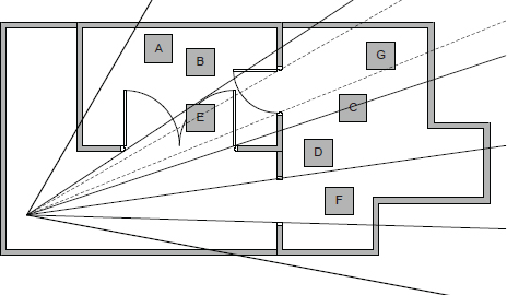

11.2.7.2 Primitive Submission
Once a list of visible geometric primitives has been generated, the individual primitives must be submitted to the GPU pipeline for rendering. This can be accomplished by making calls to DrawIndexedPrimitive() in DirectX or glDrawArrays() in OpenGL.
Render State
As we learned in Section 11.2.4, the functionality of many of the GPU pipeline’s stages is fixed but configurable. And even programmable stages are driven in part by configurable parameters. Some examples of these configurable parameters are listed below (although this is by no means a complete list):
The set of all configurable parameters within the GPU pipeline is known as the hardware state or render state. It is the application stage’s responsibility to ensure that the hardware state is configured properly and completely for each submitted primitive. Ideally these state settings are described completely by the material associated with each submesh. So the application stage’s job boils down to iterating through the list of visible mesh instances, iterating over each submesh-material pair, setting the render state based on the material’s specifications and then calling the low-level primitive submission functions (DrawIndexedPrimitive(), glDrawArrays(), or similar).
State Leaks
If we forget to set some aspect of the render state between submitted primitives, the settings used on the previous primitive will “leak” over onto the new primitive. A render state leak might manifest itself as an object with the wrong texture or an incorrect lighting effect, for example. Clearly it’s important that the application stage never allow state leaks to occur.
The GPU Command List
The application stage actually communicates with the GPU via a command list. These commands interleave render state settings with references to the geometry that should be drawn. For example, to render objects A and B with material 1, followed by objects C, D and E using material 2, the command list might look like this:
Under the hood, API functions like DrawIndexedPrimitive() actually just construct and submit GPU command lists. The cost of these API calls can themselves be too high for some applications. To maximize performance, some game engines build GPU command lists manually or by calling a low-level rendering API like Vulkan (https://www.khronos.org/vulkan/).
11.2.7.3 Geometry Sorting
Render state settings are global—they apply to the entire GPU as a whole. So in order to change render state settings, the entire GPU pipeline must be flushed before the new settings can be applied. This can cause massive performance degradation if not managed carefully.
Clearly we’d like to change render settings as infrequently as possible. The best way to accomplish this is to sort our geometry by material. That way, we can install material A’s settings, render all geometry associated with material A and then move on to material B.
Unfortunately, sorting geometry by material can have a detrimental effect on rendering performance because it increases overdraw—a situation in which the same pixel is filled multiple times by multiple overlapping triangles. Certainly some overdraw is necessary and desirable, as it is the only way to properly alpha-blend transparent and translucent surfaces into a scene. However, overdraw of opaque pixels is always a waste of GPU bandwidth.
The early z-test is designed to discard occluded fragments before the expensive pixel shader has a chance to execute. But to take maximum advantage of early z, we need to draw the triangles in front-to-back order. That way, the closest triangles will fill the z-buffer right off the bat, and all of the fragments coming from more-distant triangles behind them can be quickly discarded, with little or no overdraw.
z-Prepass to the Rescue
How can we reconcile the need to sort geometry by material with the conflicting need to render opaque geometry in a front-to-back order? The answer lies in a GPU feature known as z-prepass.
The idea behind z-prepass is to render the scene twice: the first time to generate the contents of the z-buffer as efficiently as possible and the second time to populate the frame buffer with full color information (but this time with no overdraw, thanks to the contents of the z-buffer). The GPU provides a special double-speed rendering mode in which the pixel shaders are disabled, and only the z-buffer is updated. Opaque geometry can be rendered in front-to-back order during this phase, to minimize the time required to generate the z-buffer contents. Then the geometry can be resorted into material order and rendered in full color with minimal state changes for maximum pipeline throughput.
Once the opaque geometry has been rendered, transparent surfaces can be drawn in back-to-front order. This brute-force method allows us to achieve the proper alpha-blended result. Order-independent transparency (OIT) is a technique that permits transparent geometry to be rendered in an arbitrary order. It works by storing multiple fragments per pixel, sorting each pixel’s fragments and blending them only after the entire scene has been rendered. This technique produces correct results without the need for pre-sorting the geometry, but it comes at a high memory cost because the frame buffer must be large enough to store all of the translucent fragments for each pixel.
11.2.7.4 Scene Graphs
Modern game worlds can be very large. The majority of the geometry in most scenes does not lie within the camera frustum, so frustum culling all of these objects explicitly is usually incredibly wasteful. Instead, we would like to devise a data structure that manages all of the geometry in the scene and allows us to quickly discard large swaths of the world that are nowhere near the camera frustum prior to performing detailed frustum culling. Ideally, this data structure should also help us to sort the geometry in the scene, either in front-to-back order for the z-prepass or in material order for full-color rendering.
Such a data structure is often called a scene graph, in reference to the graphlike data structures often used by film rendering engines and DCC tools like Maya. However, a game’s scene graph needn’t actually be a graph, and in fact the data structure of choice is usually some kind of tree (which is, of course, a special case of a graph). The basic idea behind most of these data structures is to partition three-dimensional space in a way that makes it easy to discard regions that do not intersect the frustum, without having to frustum cull all of the individual objects within them. Examples include quadtrees and octrees, BSP trees, kd-trees and spatial hashing techniques.
Quadtrees and Octrees
A quadtree divides space into quadrants recursively. Each level of recursion is represented by a node in the quadtree with four children, one for each quadrant. The quadrants are typically separated by vertically oriented, axis-aligned planes, so that the quadrants are square or rectangular. However, some quadtrees subdivide space using arbitrarily shaped regions.
Quadtrees can be used to store and organize virtually any kind of spatially distributed data. In the context of rendering engines, quadtrees are often used to store renderable primitives such as mesh instances, subregions of terrain geometry or individual triangles of a large static mesh, for the purposes of efficient frustum culling. The renderable primitives are stored at the leaves of the tree, and we usually aim to achieve a roughly uniform number of primitives within each leaf region. This can be achieved by deciding whether to continue or terminate the subdivision based on the number of primitives within a region.
To determine which primitives are visible within the camera frustum, we walk the tree from the root to the leaves, checking each region for intersection with the frustum. If a given quadrant does not intersect the frustum, then we know that none of its child regions will do so either, and we can stop traversing that branch of the tree. This allows us to search for potentially visible primitives much more quickly than would be possible with a linear search (usually in O(log n) time). An example of a quadtree subdivision of space is shown in Figure 11.50.
An octree is the three-dimensional equivalent of a quadtree, dividing space into eight subregions at each level of the recursive subdivision. The regions of an octree are often cubes or rectangular prisms but can be arbitrarily shaped three-dimensional regions in general.
Bounding Sphere Trees
In the same way that a quadtree or octree subdivides space into (usually) rectangular regions, a bounding sphere tree divides space into spherical regions hierarchically. The leaves of the tree contain the bounding spheres of the renderable primitives in the scene. We collect these primitives into small logical groups and calculate the net bounding sphere of each group. The groups are themselves collected into larger groups, and this process continues until we have a single group with a bounding sphere that encompasses the entire virtual world. To generate a list of potentially visible primitives, we walk the tree from the root to the leaves, testing each bounding sphere against the frustum, and only recursing down branches that intersect it.

BSP Trees
A binary space partitioning (BSP) tree divides space in half recursively until the objects within each half-space meet some predefined criteria (much as a quadtree divides space into quadrants). BSP trees have numerous uses, including collision detection and constructive solid geometry, as well as their most well-known application as a method for increasing the performance of frustum culling and geometry sorting for 3D graphics. A kd-tree is a generalization of the BSP tree concept to k dimensions.
In the context of rendering, a BSP tree divides space with a single plane at each level of the recursion. The dividing planes can be axis-aligned, but more commonly each subdivision corresponds to the plane of a single triangle in the scene. All of the other triangles are then categorized as being either on the front side or the back side of the plane. Any triangles that intersect the dividing plane are themselves divided into three new triangles, so that every triangle lies either entirely in front of or entirely behind the plane, or is coplanar with it. The result is a binary tree with a dividing plane and one or more triangles at each interior node and triangles at the leaves.
A BSP tree can be used for frustum culling in much the same way a quadtree, octree or bounding sphere tree can. However, when generated with individual triangles as described above, a BSP tree can also be used to sort triangles into a strictly back-to-front or front-to-back order. This was particularly important for early 3D games like Doom, which did not have the benefit of a z-buffer and so were forced to use the painter’s algorithm (i.e., to render the scene from back to front) to ensure proper inter-triangle occlusion.
Given a camera view point in 3D space, a back-to-front sorting algorithm walks the tree from the root. At each node, we check whether the view point is in front of or behind that node’s dividing plane. If the camera is in front of a node’s plane, we visit the node’s back children first, then draw any triangles that are coplanar with its dividing plane, and finally we visit its front children. Likewise, when the camera’s view point is found to be behind a node’s dividing plane, we visit the node’s front children first, then draw the triangles coplanar with the node’s plane and finally we visit its back children. This traversal scheme ensures that the triangles farthest from the camera will be visited before those that are closer to it, and hence it yields a back-to-front ordering. Because this algorithm traverses all of the triangles in the scene, the order of the traversal is independent of the direction the camera is looking. A secondary frustum culling step would be required in order to traverse only visible triangles. A simple BSP tree is shown in Figure 11.51, along with the tree traversal that would be done for the camera position shown.
Full coverage of BSP tree generation and usage algorithms is beyond our scope here. See http://www.gamedev.net/reference/articles/article657.asp for more details on BSP trees.
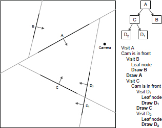
11.2.7.5 Choosing a Scene Graph
Clearly there are many different kinds of scene graphs. Which data structure to select for your game will depend upon the nature of the scenes you expect to be rendering. To make the choice wisely, you must have a clear understanding of what is required—and more importantly what is not required—when rendering scenes for your particular game.
For example, if you’re implementing a fighting game, in which two characters battle it out in a ring surrounded by a mostly static environment, you may not need much of a scene graph at all. If your game takes place primarily in enclosed indoor environments, a BSP tree or portal system may serve you well. If the action takes place outdoors on relatively flat terrain, and the scene is viewed primarily from above (as might be the case in a strategy game or god game), a simple quadtree might be all that’s required to achieve high rendering speeds. On the other hand, if an outdoor scene is viewed primarily from the point of view of someone on the ground, we may need additional culling mechanisms. Densely populated scenes can benefit from an occlusion volume (antiportal) system, because there will be plenty of occluders. On the other hand, if your outdoor scene is very sparse, adding an antiportal system probably won’t pay dividends (and might even hurt your frame rate).
Ultimately, your choice of scene graph should be based on hard data obtained by actually measuring the performance of your rendering engine. You may be surprised to learn where all your cycles are actually going! But once you know, you can select scene graph data structures and/or other optimizations to target the specific problems at hand.
11.3 Advanced Lighting and Global Illumination
In order to render photorealistic scenes, we need physically accurate global illumination algorithms. A complete coverage of these techniques is beyond our scope. In the following sections, we will briefly outline the most prevalent techniques in use within the game industry today. Our goal here is to provide you with an awareness of these techniques and a jumping-off point for further investigation. For an excellent in-depth coverage of this topic, see [10].
11.3.1 Image-Based Lighting
A number of advanced lighting and shading techniques make heavy use of image data, usually in the form of two-dimensional texture maps. These are called image-based lighting algorithms.

11.3.1.1 Normal Mapping
A normal map specifies a surface normal direction vector at each texel. This allows a 3D modeler to provide the rendering engine with a highly detailed description of a surface’s shape, without having to tessellate the model to a high degree (as would be required if this same information were to be provided via vertex normals). Using a normal map, a single flat triangle can be made to look as though it were constructed from millions of tiny triangles. An example of normal mapping is shown in Figure 11.52.
The normal vectors are typically encoded in the RGB color channels of the texture, with a suitable bias to overcome the fact that RGB channels are strictly positive while normal vector components can be negative. Sometimes only two coordinates are stored in the texture; the third can be easily calculated at runtime, given the assumption that the surface normals are unit vectors.
11.3.1.2 Heightmaps: Bump, Parallax and Displacement Mapping
As its name implies, a heightmap encodes the height of the ideal surface above or below the surface of the triangle. Heightmaps are typically encoded as grayscale images, since we only need a single height value per texel. Height-maps can be used for bump mapping, parallax occlusion mapping and displacement mapping—three techniques that can make a planar surface appear to have height variation.
In bump mapping, a heightmap is used as a cheap way to generate surface normals. This technique was primarily used in the early days of 3D graphics—nowadays, most game engines store surface normal information explicitly in a normal map, rather than calculating the normals from a height-map.

Parallax occlusion mapping uses the information in a heightmap to artificially adjust the texture coordinates used when rendering a flat surface, in such a way as to make the surface appear to contain surface details that move semi-correctly as the camera moves. (This technique was used to produce the bullet impact decals in the Uncharted series of games by Naughty Dog.)
Displacement mapping (also known as relief mapping) produces real surface details by actually tessellating and then extruding surface polygons, again using a heightmap to determine how much to displace each vertex. This produces the most convincing effect—one that properly self-occludes and self-shadows—because real geometry is being generated. Figure 11.53 compares bump mapping, parallax mapping and displacement mapping. Figure 11.54 shows an example of displacement mapping implemented in DirectX 9.
11.3.1.3 Specular/Gloss Maps
When light reflects directly off a shiny surface, we call this specular reflection. The intensity of a specular reflection depends on the relative angles of the viewer, the light source and the surface normal. As we saw in Section 11.1.3.2, the specular intensity takes the form kS(R · V)α, where R is the reflection of the light’s direction vector about the surface normal, V is the direction to the viewer, kS is the overall specular reflectivity of the surface and α is called the specular power.
Many surfaces aren’t uniformly glossy. For example, when a person’s face is sweaty and dirty, wet regions appear shiny, while dry or dirty areas appear dull. We can encode high-detail specularity information in a special texture map known as a specular map.
If we store the value of kS in the texels of a specular map, we can control how much specular reflection should be applied at each texel. This kind of specular map is sometimes called a gloss map. It is also called a specular mask, because zero-valued texels can be used to “mask off” regions of the surface where we do not want specular reflection applied. If we store the value of α in our specular map, we can control the amount of “focus” our specular highlights will have at each texel. This kind of texture is called a specular power map. An example of a gloss map is shown in Figure 11.55.

11.3.1.4 Environment Mapping
An environment map looks like a panoramic photograph of the environment taken from the point of view of an object in the scene, covering a full 360 degrees horizontally and either 180 degrees or 360 degrees vertically. An environment map acts like a description of the general lighting environment surrounding an object. It is generally used to inexpensively render reflections.
The two most common formats are spherical environment maps and cubic environment maps. A spherical map looks like a photograph taken through a fisheye lens, and it is treated as though it were mapped onto the inside of a sphere whose radius is infinite, centered about the object being rendered. The problem with sphere maps is that they are addressed using spherical coordinates. Around the equator, there is plenty of resolution both horizontally and vertically. However, as the vertical (azimuthal) angle approaches vertical, the resolution of the texture along the horizontal (zenith) axis decreases to a single texel. Cube maps were devised to avoid this problem.

A cube map looks like a composite photograph pieced together from photos taken in the six primary directions (up, down, left, right, front and back). During rendering, a cube map is treated as though it were mapped onto the six inner surfaces of a box at infinity, centered on the object being rendered.
To read the environment map texel corresponding to a point P on the surface of an object, we take the ray from the camera to the point P and reflect it about the surface normal at P. The reflected ray is followed until it intersects the sphere or cube of the environment map. The value of the texel at this intersection point is used when shading the point P.
11.3.1.5 Three-Dimensional Textures
Modern graphics hardware also includes support for three-dimensional textures. A 3D texture can be thought of as a stack of 2D textures. The GPU knows how to address and filter a 3D texture, given a three-dimensional texture coordinate (u, v, w).
Three-dimensional textures can be useful for describing the appearance or volumetric properties of an object. For example, we could render a marble sphere and allow it to be cut by an arbitrary plane. The texture would look continuous and correct across the cut no matter where it was made, because the texture is well-defined and continuous throughout the entire volume of the sphere.
11.3.2 High Dynamic Range Lighting
A display device like a television set or CRT monitor can only produce a limited range of intensities. This is why the color channels in the frame buffer are limited to a zero to one range. But in the real world, light intensities can grow arbitrarily large. High dynamic range (HDR) lighting attempts to capture this wide range of light intensities.
HDR lighting performs lighting calculations without clamping the resulting intensities arbitrarily. The resulting image is stored in a format that permits intensities to grow beyond one. The net effect is an image in which extreme dark and light regions can be represented without loss of detail within either type of region.
Prior to display on-screen, a process called tone mapping is used to shift and scale the image’s intensity range into the range supported by the display device. Doing this permits the rendering engine to reproduce many real-world visual effects, like the temporary blindness that occurs when you walk from a dark room into a brightly lit area, or the way light seems to bleed out from behind a brightly back-lit object (an effect known as bloom).
One way to represent an HDR image is to store the R, G and B channels using 32-bit floating-point numbers, instead of 8-bit integers. Another alternative is to employ an entirely different color model altogether. The log-LUV color model is a popular choice for HDR lighting. In this model, color is represented as an intensity channel (L) and two chromaticity channels (U and V). Because the human eye is more sensitive to changes in intensity than it is to changes in chromaticity, the L channel is stored in 16 bits while U and V are given only eight bits each. In addition, L is represented using a logarithmic scale (base two) in order to capture a very wide range of light intensities.
11.3.3 Global Illumination
As we noted in Section 11.1.3.1, global illumination refers to a class of lighting algorithms that account for light’s interactions with multiple objects in the scene, on its way from the light source to the virtual camera. Global illumination accounts for effects like the shadows that arise when one surface occludes another, reflections, caustics and the way the color of one object can “bleed” onto the objects around it. In the following sections, we’ll take a brief look at some of the most common global illumination techniques. Some of these methods aim to reproduce a single isolated effect, like shadows or reflections. Others like radiosity and ray tracing methods aim to provide a holistic model of global light transport.
11.3.3.1 Shadow Rendering
Shadows are created when a surface blocks light’s path. The shadows caused by an ideal point light source would be sharp, but in the real world shadows have blurry edges; this is called the penumbra. A penumbra arises because real-world light sources cover some area and so produce light rays that graze the edges of an object at different angles.
The two most prevalent shadow rendering techniques are shadow volumes and shadow maps. We’ll briefly describe each in the sections below. In both techniques, objects in the scene are generally divided into three categories: objects that cast shadows, objects that are to receive shadows and objects that are entirely excluded from consideration when rendering shadows. Likewise, the lights are tagged to indicate whether or not they should generate shadows. This important optimization limits the number of light-object combinations that need to be processed in order to produce the shadows in a scene.
Shadow Volumes
In the shadow volume technique, each shadow caster is viewed from the vantage point of a shadow-generating light source, and the shadow caster’s silhouette edges are identified. These edges are extruded in the direction of the light rays emanating from the light source. The result is a new piece of geometry that describes the volume of space in which the light is occluded by the shadow caster in question. This is shown in Figure 11.56.
A shadow volume is used to generate a shadow by making use of a special full-screen buffer known as the stencil buffer. This buffer stores a single integer value corresponding to each pixel of the screen. Rendering can be masked by the values in the stencil buffer—for example, we could configure the GPU to only render fragments whose corresponding stencil values are nonzero. In addition, the GPU can be configured so that rendered geometry updates the values in the stencil buffer in various useful ways.
To render shadows, the scene is first drawn to generate an unshadowed image in the frame buffer, along with an accurate z-buffer. The stencil buffer is cleared so that it contains zeros at every pixel. Each shadow volume is then rendered from the point of view of the camera in such a way that front-facing triangles increase the values in the stencil buffer by one, while back-facing triangles decrease them by one. In areas of the screen where the shadow volume does not appear at all, of course the stencil buffer’s pixels will be left containing zero. The stencil buffer will also contain zeros where both the front and back faces of the shadow volume are visible, because the front face will increase the stencil value but the back face will decrease it again. In areas where the back face of the shadow volume has been occluded by “real” scene geometry, the stencil value will be one. This tells us which pixels of the screen are in shadow. So we can render shadows in a third pass, by simply darkening those regions of the screen that contain a nonzero stencil buffer value.
Shadow Maps
The shadow mapping technique is effectively a per-fragment depth test performed from the point of view of the light instead of from the point of view of the camera. The scene is rendered in two steps: First, a shadow map texture is generated by rendering the scene from the point of view of the light source and saving off the contents of the depth buffer. Second, the scene is rendered as usual, and the shadow map is used to determine whether or not each fragment is in shadow. At each fragment in the scene, the shadow map tells us whether or not the light is being occluded by some geometry that is closer to the light source, in just the same way that the z-buffer tells us whether a fragment is being occluded by a triangle that is closer to the camera.
A shadow map contains only depth information—each texel records how far away it is from the light source. Shadow maps are therefore typically rendered using the hardware’s double-speed z-only mode (since all we care about is the depth information). For a point light source, a perspective projection is used when rendering the shadow map; for a directional light source, an orthographic projection is used instead.

To render a scene using a shadow map, we draw the scene as usual from the point of view of the camera. For each vertex of every triangle, we calculate its position in light space—i.e., in the same “view space” that was used when generating the shadow map in the first place. These light-space coordinates can be interpolated across the triangle, just like any other vertex attribute. This gives us the position of each fragment in light space. To determine whether a given fragment is in shadow or not, we convert the fragment’s light-space (x, y)-coordinates into texture coordinates (u, v) within the shadow map. We then compare the fragment’s light-space z-coordinate with the depth stored at the corresponding texel in the shadow depth map. If the fragment’s lightspace z is farther away from the light than the texel in the shadow map, then it must be occluded by some other piece of geometry that is closer to the light source—hence it is in shadow. Likewise, if the fragment’s light-space z is closer to the light source than the texel in the shadow map, then it is not occluded and is not in shadow. Based on this information, the fragment’s color can be adjusted accordingly. The shadow mapping process is illustrated in Figure 11.57.
11.3.3.2 Ambient Occlusion
Ambient occlusion is a technique for modeling contact shadows—the soft shadows that arise when a scene is illuminated by only ambient light. In effect, ambient occlusion describes how “accessible” each point on a surface is to light in general. For example, the interior of a section of pipe is less accessible to ambient light than its exterior. If the pipe were placed outside on an overcast day, its interior would generally appear darker than its exterior.
Figure 11.58 shows how ambient occlusion produces shadows underneath a car and in its wheel wells, as well as within the seams between body panels. Ambient occlusion is measured at a point on a surface by constructing a hemisphere with a very large radius centered on that point and determing what percentage of that hemisphere’s area is visible from the point in question. It can be precomputed offline for static objects, because ambient occlusion is independent of view direction and the direction of incident light. It is typically stored in a texture map that records the level of ambient occlusion at each texel across the surface.

11.3.3.3 Reflections
Reflections occur when light bounces off a highly specular (shiny) surface producing an image of another portion of the scene in the surface. Reflections can be implemented in a number of ways. Environment maps are used to produce general reflections of the surrounding environment on the surfaces of shiny objects. Direct reflections in flat surfaces like mirrors can be produced by reflecting the camera’s position about the plane of the reflective surface and then rendering the scene from that reflected point of view into a texture. The texture is then applied to the reflective surface in a second pass (see Figure 11.59).
11.3.3.4 Caustics
Caustics are the bright specular highlights arising from intense reflections or refractions from very shiny surfaces like water or polished metal. When the reflective surface moves, as is the case for water, the caustic effects glimmer and “swim” across the surfaces on which they fall. Caustic effects can be produced by projecting a (possibly animated) texture containing semi-random bright highlights onto the affected surfaces. An example of this technique is shown in Figure 11.60.
11.3.3.5 Subsurface Scattering
When light enters a surface at one point, is scattered beneath the surface, and then reemerges at a different point on the surface, we call this subsurface scattering. This phenomenon is responsible for the “warm glow” of human skin, wax and marble statues (e.g., Figure 11.61). Subsurface scattering is described by a more-advanced variant of the BRDF (see Section 11.1.3.2) known as the BSSRDF (bidirectional surface scattering reflectance distribution function).
Subsurface scattering can be simulated in a number of ways. Depth-map-based subsurface scattering renders a shadow map (see Section 11.3.3.1), but instead of using it to determine which pixels are in shadow, it is used to measure how far a beam of light would have to travel in order to pass all the way through the occluding object. The shadowed side of the object is then given an artificial diffuse lighting term whose intensity is inversely proportional to the distance the light had to travel in order to emerge on the opposite side of the object. This causes objects to appear to be glowing slightly on the side opposite to the light source but only where the object is relatively thin. For more information on subsurface scattering techniques, see http://http.developer.nvidia.com/GPUGems/gpugems_ch16.html.

11.3.3.6 Precomputed Radiance Transfer (PRT)
Precomputed radiance transfer (PRT) is a popular technique that attempts to simulate the effects of radiosity-based rendering methods in real time. It does so by precomputing and storing a complete description of how an incident light ray would interact with a surface (reflect, refract, scatter, etc.) when approaching from every possible direction. At runtime, the response to a particular incident light ray can be looked up and quickly converted into very accurate lighting results.
In general the light’s response at a point on the surface is a complex function defined on a hemisphere centered about the point. A compact representation of this function is required to make the PRT technique practical. A common approach is to approximate the function as a linear combination of spherical harmonic basis functions. This is essentially the three-dimensional equivalent of encoding a simple scalar function f(x) as a linear combination of shifted and scaled sine waves.
The details of PRT are far beyond our scope. For more information, see http://web4.cs.ucl.ac.uk/staff/j.kautz/publications/prtSIG02.pdf. PRT lighting techniques are demonstrated in a DirectX sample program available in the DirectX SDK—see http://msdn.microsoft.com/en-us/library/bb147287.aspx for more details.
11.3.4 Deferred Rendering
In traditional triangle-rasterization–based rendering, all lighting and shading calculations are performed on the triangle fragments in world space, view space or tangent space. The problem with this technique is that it is inherently inefficient. For one thing, we potentially do work that we don’t need to do. We shade the vertices of triangles, only to discover during the rasterization stage that the entire triangle is being depth-culled by the z-test. Early z-tests help eliminate unnecessary pixel shader evaluations, but even this isn’t perfect. What’s more, in order to handle a complex scene with lots of lights, we end up with a proliferation of different versions of our vertex and pixel shaders—versions that handle different numbers of lights, different types of lights, different numbers of skinning weights, etc.
Deferred rendering is an alternative way to shade a scene that addresses many of these problems. In deferred rendering, the majority of the lighting calculations are done in screen space, not view space. We efficiently render the scene without worrying about lighting. During this phase, we store all the information we’re going to need to light the pixels in a “deep” frame buffer known as the G-buffer. Once the scene has been fully rendered, we use the information in the G-buffer to perform our lighting and shading calculations. This is usually much more efficient than view-space lighting, avoids the proliferation of shader variants and permits some very pleasing effects to be rendered relatively easily.
The G-buffer may be physically implemented as a collection of buffers, but conceptually it is a single frame buffer containing a rich set of information about the lighting and surface properties of the objects in the scene at every pixel on the screen. A typical G-buffer might contain the following perpixel attributes: depth, surface normal in view space or world space, diffuse color, specular power, even precomputed radiance transfer (PRT) coefficients. The following sequence of screenshots from Guerrilla Games’ Killzone 2 (Figure 11.62) shows some of the typical components of the G-buffer.
An in-depth discussion of deferred rendering is beyond our scope, but the folks at Guerrilla Games have prepared an excellent presentation on the topic, which is available at http://www.slideshare.net/guerrillagames/deferred-rendering-in-killzone-2-9691589.
11.3.5 Physically Based Shading
Traditional game lighting engines have required artists and lighters to tweak a wide variety of sometimes non-intuitive parameters, across numerous disparate rendering engine systems, in order to achieve a desired “look” in-game. This can be an arduous and time-consuming process. What’s worse, parameter settings that work well under one set of lighting conditions might not work well under other lighting scenarios. To address these problems, rendering programmers are turning toward physically based shading models.

A physically based shading model attempts to approximate the ways in which light travels and interacts with materials in the real world, allowing artists and lighters to tweak shader parameters using intuitive, real-world quantities measured in real-world units. A complete discussion of physically based shading is beyond the scope of this book, but you can start to learn more about it here: https://www.marmoset.co/toolbag/learn/pbr-theory.
11.4 Visual Effects and Overlays
The rendering pipeline we’ve discussed to this point is responsible primarily for rendering three-dimensional solid objects. A number of specialized rendering systems are typically layered on top of this pipeline, responsible for rendering visual elements like particle effects, decals (small geometry overlays that represent bullet holes, cracks, scratches and other surface details), hair and fur, rain or falling snow, water and other specialized visual effects. Full-screen post effects may be applied, including vignette (a reduction of brightness and saturation around the edges of the screen), motion blur, depth of field blurring, artificial/enhanced colorization, and the list goes on. Finally, the game’s menu system and heads-up display (HUD) are typically realized by rendering text and other two- or three-dimensional graphics in screen space overlaid on top of the three-dimensional scene.
An in-depth coverage of these engine systems is beyond our scope. In the following sections, we’ll provide a brief overview of these rendering systems, and point you in the direction of additional information.
11.4.1 Particle Effects
A particle rendering system is concerned with rendering amorphous objects like clouds of smoke, sparks, flame and so on. These are called particle effects. The key features that differentiate a particle effect from other kinds of renderable geometry are as follows:
Particle effects could be rendered using regular triangle mesh geometry with appropriate shaders. However, because of the unique characteristics listed above, a specialized particle effect animation and rendering system is always used to implement them in a real production game engine. A few example particle effects are shown in Figure 11.63.
Particle system design and implementation is a rich topic that could occupy many chapters all on its own. For more information on particle systems, see [2, Section 10.7], [16, Section 20.5], [11, Section 13.7] and [12, Section 4.1.2].
11.4.2 Decals
A decal is a relatively small piece of geometry that is overlaid on top of the regular geometry in the scene, allowing the visual appearance of the surface to be modified dynamically. Examples include bullet holes, foot prints, scratches, cracks, etc.
The approach most often used by modern engines is to model a decal as a rectangular area that is to be projected along a ray into the scene. This gives rise to a rectangular prism in 3D space. Whatever surface the prism intersects first becomes the surface of the decal. The triangles of the intersected geometry are extracted and clipped against the four bounding planes of the decal’s projected prism. The resulting triangles are texture-mapped with a desired decal texture by generating appropriate texture coordinates for each vertex. These texture-mapped triangles are then rendered over the top of the regular scene, often using parallax mapping to give them the illusion of depth and with a slight z-bias (usually implemented by shifting the near plane slightly) so they don’t experience z-fighting with the geometry on which they are overlaid. The result is the appearance of a bullet hole, scratch or other kind of surface modification. Some bullet-hole decals are depicted in Figure 11.64.
For more information on creating and rendering decals, see [9, Section 4.8] and [32, Section 9.2].

11.4.3 Environmental Effects
Any game that takes place in a somewhat natural or realistic environment requires some kind of environmental rendering effects. These effects are usually implemented via specialized rendering systems. We’ll take a brief look at a few of the more common of these systems in the following sections.
11.4.3.1 Skies
The sky in a game world needs to contain vivid detail, yet technically speaking it lies an extremely long distance away from the camera. Therefore, we cannot model it as it really is and must turn instead to various specialized rendering techniques.
One simple approach is to fill the frame buffer with the sky texture prior to rendering any 3D geometry. The sky texture should be rendered at an approximate 1:1 texel-to-pixel ratio, so that the texture is roughly or exactly the resolution of the screen. The sky texture can be rotated and scrolled to correspond to the motions of the camera in-game. During rendering of the sky, we make sure to set the depth of all pixels in the frame buffer to the maximum possible depth value. This ensures that the 3D scene elements will always sort on top of the sky. The arcade hit Hydro Thunder rendered its skies in exactly this manner.
On modern game platforms, where pixel shading costs can be high, sky rendering is often done after the rest of the scene has been rendered. First the z-buffer is cleared to the maximum z-value. Then the scene is rendered. Finally the sky is rendered, with z-testing enabled, z writing turned off, and using a z-test value that is one less than the maximum. This causes the sky to be drawn only where it is not occluded by closer objects like terrain, buildings and trees. Drawing the sky last ensures that its pixel shader is run for the minimum possible number of screen pixels.
For games in which the player can look in any direction, we can use a sky dome or sky box. The dome or box is rendered with its center always at the camera’s current location, so that it appears to lie at infinity, no matter where the camera moves in the game world. As with the sky texture approach, the sky box or dome is rendered before any other 3D geometry, and all of the pixels in the frame buffer are set to the maximum z-value when the sky is rendered. This means that the dome or box can actually be tiny, relative to other objects in the scene. Its size is irrelevant, as long as it fills the entire frame buffer when it is drawn. For more information on sky rendering, see [2, Section 10.3] and [44, page 253].
Clouds are often implemented with a specialized rendering and animation system as well. In early games like Doom and Quake, the clouds were just planes with scrolling semitransparent cloud textures on them. More-recent cloud techniques include camera-facing cards (billboards), particle-effect based clouds and volumetric cloud effects.
11.4.3.2 Terrain
The goal of a terrain system is to model the surface of the earth and provide a canvas of sorts upon which other static and dynamic elements can be laid out. Terrain is sometimes modeled explicitly in a package like Maya. But if the player can see far into the distance, we usually want some kind of dynamic tessellation or other level of detail (LOD) system. We may also need to limit the amount of data required to represent very large outdoor areas.
Height field terrain is one popular choice for modeling large terrain areas. The data size can be kept relatively small because a height field is typically stored in a grayscale texture map. In most height-field– based terrain systems, the horizontal (y = 0) plane is tessellated in a regular grid pattern, and the heights of the terrain vertices are determined by sampling the height field texture. The number of triangles per unit area can be varied based on distance from the camera, thereby allowing large-scale features to be seen in the distance, while still permitting a good deal of detail to be represented for nearby terrain. An example of a terrain defined via a height field bitmap is shown in Figure 11.65.
Terrain systems usually provide specialized tools for “painting” the height field itself, carving out terrain features like roads, rivers and so on. Texture mapping in a terrain system is often a blend between four or more textures. This allows artists to “paint” in grass, dirt, gravel and other terrain features by simply exposing one of the texture layers. The layers can be cross-blended from one to another to provide smooth textural transitions. Some terrain tools also permit sections of the terrain to be cut out to permit buildings, trenches and other specialized terrain features to be inserted in the form of regular mesh geometry. Terrain authoring tools are sometimes integrated directly into the game world editor, while in other engines they may be stand-alone tools.

Of course, height field terrain is just one of many options for modeling the surface of the Earth in a game. For more information on terrain rendering, see [8, Sections 4.16 through 4.19] and [9, Section 4.2].
11.4.3.3 Water
Water renderers are commonplace in games nowadays. There are lots of different kinds of water, including oceans, pools, rivers, waterfalls, fountains, jets, puddles and damp solid surfaces. Each type of water generally requires some specialized rendering technology. Some also require dynamic motion simulations. Large bodies of water may require dynamic tessellation or other LOD methodologies similar to those employed in a terrain system.
Water systems sometimes interact with a game’s rigid body dynamics system (flotation, force from water jets, etc.) and with gameplay (slippery surfaces, swimming mechanics, diving mechanics, riding vertical jets of water and so on). Water effects are often created by combining disparate rendering technologies and subsystems. For example, a waterfall might make use of specialized water shaders, scrolling textures, particle effects for mist at the base, a decal-like overlay for foam, and the list goes on. Today’s games offer some pretty amazing water effects, and active research into technologies like real-time fluid dynamics promises to make water simulations even richer and more realistic in the years ahead. For more information on water rendering and simulation techniques, see [2, Sections 9.3, 9.5 and 9.6], [15] and [8, Sections 2.6 and 5.11].
11.4.4 Overlays
Most games have heads-up displays, in-game graphical user interfaces and menu systems. These overlays are typically comprised of two- and three-dimensional graphics rendered directly in view space or screen space.
Overlays are generally rendered after the primary scene, with z-testing disabled to ensure that they appear on top of the three-dimensional scene. Two-dimensional overlays are typically implemented by rendering quads (triangle pairs) in screen space using an orthographic projection. Three-dimensional overlays may be rendered using an orthographic projection or via the regular perspective projection with the geometry positioned in view space so that it follows the camera around.
11.4.4.1 Text and Fonts
A game engine’s text/font system is typically implemented as a special kind of two-dimensional (or sometimes three-dimensional) overlay. At its core, a text rendering system needs to be capable of displaying a sequence of character glyphs corresponding to a text string, arranged in various orientations on the screen.
A font is often implemented via a texture map known as a glyph atlas, which contains the various required glyphs. This texture typically consists of a single alpha channel—the value at each pixel representing the percentage of that pixel that is covered by the interior of a glyph. A font description file provides information such as the bounding boxes of each glyph within the texture, and font layout information such as kerning, baseline offsets and so on. A glyph is rendered by drawing a quad whose (u, v) coordinates correspond to the bounding box of the desired glyph within the atlas texture map. The texture map provides the alpha value, while the color is specified separately, allowing glyphs of any color to be rendered from the same atlas.
Another option for font rendering is to make use of a font library like FreeType (https://www.freetype.org/). The FreeType library enables a game or other application to read fonts in a wide variety of formats, including TrueType (TTF) and OpenType (OTF), and to render glyphs into in-memory pixmaps at any desired point size. FreeType renders each glyph using its Bezier curve outlines, so it produces very accurate results.
Typically a real-time application like a game will use FreeType to prerender the necessary glyphs into an atlas, which is in turn used as a texture map to render glyphs as simple quads every frame. However, by embedding FreeType or a similar library in your engine, it’s possible to render some glyphs into the atlas on the fly, on an as-needed basis. This can be useful when rendering text in a language with a very large number of possible glyphs, like Chinese or Korean.
Yet another way to render high-quality character glyphs is to use signed distance fields to describe the glyphs. In this approach, glyphs are rendered to pixmaps (as they would be with a library like FreeType), but the value at each pixel is no longer an alpha “coverage” value. Instead, each pixel contains a signed distance from that pixel center to the nearest edge of the glyph. Inside the glyph, the distances are negative; outside the glyph’s outlines, they are positive. When rendering a glyph from a signed distance field texture atlas, the distances are used in the pixel shader to calculate highly accurate alpha values. The net result is text that looks smooth at any distance or viewing angle. You can read more about signed distance field text rendering by searching online for Konstantin Käfer’s article entitled “Drawing Text with Signed Distance Fields in Mapbox GL,” or the article written by Chris Green of Valve entitled “Improved Alpha-Tested Magnification for Vector Textures and Special Effects.”
Glyphs can also be rendered directly from the Bézier curve outlines that define them. The Slug font rendering library by Terathon Software LLC performs its outline-based glyph rendering on the GPU, thereby making this technique practical for use in a real-time game application.
A good text/font system must account for the differences in character sets and reading directions inherent in various languages. Laying out the characters in a text string is a process known as shaping the string. The characters are laid out from left to right or right to left, depending on the language, with each character aligned to a common baseline. The spacing between characters is determined in part by metrics provided by the creator of the font (and stored in the font file), and partly by kerning rules that dictate contextual intercharacter spacing adjustments.
Some text systems also provide various fun features like the ability to animate characters across the screen in various ways, the ability to animate individual characters and so on. However, it’s important to remember when implementing a game font system that only those features that are actually required by the game should be implemented. There’s no point in furnishing your engine with an advanced text animation if your game never needs to display animated text, for example.

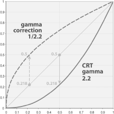
11.4.5 Gamma Correction
CRT monitors tend to have a nonlinear response to luminance values. That is, if a linearly increasing ramp of R, G or B values were to be sent to a CRT, the image that would result on-screen would be perceptually nonlinear to the human eye. Visually, the dark regions of the image would look darker than they should. This is illustrated in Figure 11.66.
The gamma response curve of a typical CRT display can be modeled quite simply by the formula
where γCRT > 1. To correct for this effect, the colors sent to the CRT display are usually passed through an inverse transformation (i.e., using a gamma value γcorr < 1). The value of γCRT for a typical CRT monitor is 2.2, so the correction value is usually γcorr ≈ 1/2.2 = 0.455. These gamma encoding and decoding curves are shown in Figure 11.67.
Gamma encoding can be performed by the 3D rendering engine to ensure that the values in the final image are properly gamma-corrected. One problem that is encountered, however, is that the bitmap images used to represent texture maps are often gamma-corrected themselves. A high-quality rendering engine takes this fact into account, by gamma-decoding the textures prior to rendering and then re-encoding the gamma of the final rendered scene so that its colors can be reproduced properly on-screen.
11.4.6 Full-Screen Post Effects
Full-screen post effects are effects applied to a rendered three-dimensional scene that provide additional realism or a stylized look. These effects are often implemented by passing the entire contents of the screen through a pixel shader that applies the desired effect(s). This can be accomplished by rendering a full-screen quad that has been mapped with a texture containing the unfiltered scene. A few examples of full-screen post effects are given below:
11.5 Further Reading
We’ve covered a lot of material in a very short space in this chapter, but we’ve only just scratched the surface. No doubt you’ll want to explore many of these topics in much greater detail. For an excellent overview of the entire process of creating three-dimensional computer graphics and animation for games and film, I highly recommend [27]. The technology that underlies modern realtime rendering is covered in excellent depth in [2], while [16] is well known as the definitive reference guide to all things related to computer graphics. Other great books on 3D rendering include [49], [11] and [12]. The mathematics of 3D rendering is covered very well in [32]. No graphics programmer’s library would be complete without one or more books from the Graphics Gems series ([20], [5], [28], [22] and [42]) and/or the GPU Gems series ([15], [44] and [40]). Of course, this short reference list is only the beginning—you will undoubtedly encounter a great many more excellent books on rendering and shaders over the course of your career as a game programmer.