
Signal Representation and Modeling
Chapter Objectives
- Understand the concept of a signal and how to work with mathematical models of signals.
- Discuss fundamental signal types and signal operations used in the study of signals and systems. Experiment with methods of simulating continuous- and discrete-time signals with MATLAB.
- Learn various ways of classifying signals and discuss symmetry properties.
- Explore characteristics of sinusoidal signals. Learn phasor representation of sinusoidal signals, and how phasors help with analysis.
- Understand the decomposition of signals using unit-impulse functions of appropriate type.
- Learn energy and power definitions.
1.1 Introduction
Signals are part of our daily lives. We work with a wide variety of signals on a day-today basis whether we realize it or not. When a commentator in a radio broadcast studio speaks into a microphone, the sound waves create changes in the air pressure around the microphone. If we happen to be in the same studio, membranes in our ears detect the changes in the air pressure, and we perceive them as sound. Pressure changes also cause vibrations on the membrane within the microphone. In response, the microphone produces a time-varying electrical voltage in such a way that the variations of the electrical voltage mimic the variations of air pressure in the studio. Thus, the microphone acts as a transducer which converts an acoustic signal to an electrical signal. This is just one step in the process of radio broadcast. The electrical signal produced by a microphone is modified and enhanced in a variety of ways, and its strength is boosted. It is then applied to a transmitting antenna which converts it to an electromagnetic signal that is suitable for transmission over the air for long distances. These electromagnetic waves fill the air space that we live in. An electromagnetic signal picked up by the antenna of a radio receiver is converted back to the form of an electrical voltage signal which is further processed within the radio receiver and sent to a loudspeaker. The loudspeaker converts this electrical voltage signal to vibrations which recreate the air pressure variations similar to those that started the whole process at the broadcast studio.
The broadcast example discussed above includes acoustic, electrical and electromagnetic signals. Examples of different physical signals can also be found around us. Time variations of quantities such as force, torque, speed and acceleration can be taken as examples of mechanical signals. For example, in an automobile, a tachometer measures the speed of the vehicle as a signal, and produces an electrical voltage the strength of which is proportional to the speed at each time instant. Subsequently, the electrical signal produced by the tachometer can be used in a speed control system to regulate the speed of the vehicle.
Consider a gray-scale photograph printed from a film negative obtained using an old film camera. Each point on the photograph has a shade of gray ranging from pure black to pure white. If we can represent shades of gray numerically, say with values ranging from 0.0 to 1.0, then the photograph can be taken as a signal. In this case, the strength of each point is not a function of time, but rather a function of horizontal and vertical distances from a reference point such as the bottom left corner of the photograph. If a digital camera is to be used to capture an image, the resulting signal is slightly different. The sensor of a digital camera is made up of photo-sensitive cells arranged in a rectangular grid pattern. Each cell measures the intensity of light it receives, and produces a voltage that is proportional to it. Thus, the signal that represents a digital image also consists of light intensity values as a function of horizontal and vertical distances. The difference is that, due to the finite number of cells on the sensor, only the distance values that are multiples of cell width and cell height are meaningful. Light intensity information only exists for certain values of the distance, and is undefined between them.
Examples of signals can also be found outside engineering disciplines. Financial markets, for example, rely on certain economic indicators for investment decisions. One such indicator that is widely used is the Dow Jones Industrial Average (DJIA) which is computed as a weighted average of the stock prices of 30 large publicly owned companies. Day-to-day variations of the DJIA can be used by investors in assessing the health of the economy and in making buying or selling decisions.
1.2 Mathematical Modeling of Signals
In the previous section we have discussed several examples of signals that we encounter on a day-to-day basis. These signals are in one or another physical form; some are electrical signals, some are in the form of air pressure variations over time, some correspond to time variations of a force or a torque in a mechanical system, and some represent light intensity and/or color as a function of horizontal and vertical distance from a reference point. There are other physical forms as well. In working with signals, we have one or both of the following goals in mind:
Understand the characteristics of the signal in terms of its behavior in time and in terms of the frequencies it contains (signal analysis).
For example, consider the electrical signal produced by a microphone. Two people uttering the same word into the microphone do not necessarily produce the same exact signal. Would it be possible to recognize the speaker from his or her signal? Would it be possible to identify the spoken word?
Develop methods of creating signals with desired characteristics (signal synthesis). Consider an electronic keyboard that synthesizes sounds of different musical instruments such as the piano and the violin. Naturally, to create the sound of either instrument we need to understand the characteristics of the sounds these instruments make. Other examples are the synthesis of human speech from printed text by text-to-speech software and the synthesis of test signals in a laboratory for testing and calibrating specialized equipment.
In addition, signals are often used in conjunction with systems. A signal is applied to a system as input, and the system responds to the signal by producing another signal called the output. For example, the signal from an electric guitar can be applied (connected via cable) to a system that boosts its strength or enhances the sound acoustically. In problems that involve the interaction of a signal with a system we may have additional goals:
3. Understand how a system responds to a signal and why (system analysis).
What characteristics of the input signal does the system retain from its input to its output? What characteristics of the input signal are modified by the system, and in what ways?
4. Develop methods of constructing a system that responds to a signal in some prescribed way (system synthesis).
Understanding different characteristics of signals will also help us in the design of systems that affect signals in desired ways. An example is the design of a system to enhance the sound of a guitar and give it the ”feel” of being played in a concert hall with certain acoustic properties. Another example is the automatic speed control system of an automobile that is required to accelerate or decelerate automobile to the desired speed within prescribed constraints.
In analyzing signals of different physical forms we need to develop a uniform framework. It certainly would not be practical to devise different analysis methods for different types of physical signals. Therefore, we work with mathematical models of physical signals.
Most of the examples utilized in our discussion so far involved signals in the form of a physical quantity varying over time. There are exceptions; some signals could be in the form of variations of a physical quantity over a spatial variable. Examples of this are the distribution of force along the length of a steel beam, or the distribution of light intensity at different points in an image. To simplify the discussion, we will focus our attention on signals that are functions of time. The techniques that will be developed are equally applicable to signals that use other independent variables as well.
The mathematical model for a signal is in the form of a formula, function, algorithm or a graph that approximately describes the time variations of the physical signal.
1.3 Continuous-Time Signals
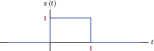
Consider x(t), a mathematical function of time chosen to approximate the strength of the physical quantity at the time instant t. In this relationship t is the independent variable, and x is the dependent variable. The signal x(t) is referred to as a continuous-time signal or an analog signal. An example of a continuous-time signal is shown in Fig. 1.1.
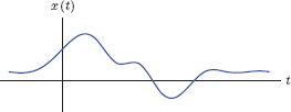
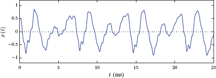
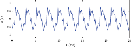
Fig. 1.2 illustrates the mathematical model for a 25 ms segment of the voice signal that corresponds to the vowel “o” in the word “hello”. Similarly, a 25 ms segment of the sound from a violin playing the note A3 is shown in Fig. 1.3.
Some signals can be described analytically. For example, the function
x(t)=5sin(12t)
describes a sinusoidal signal. Sometimes it is convenient to describe a signal model by patching together multiple signal segments, each modeled with a different function. An example of this is
x(t)={e-3t-e-6t,t≥00,t<0
Software resources: |
See MATLAB Exercise 1.1. |
1.3.1 Signal operations
In this section we will discuss time-domain operations that are commonly used in the course of working with continuous-time signals. Some are simple arithmetic operators. Examples of these are addition and multiplication of signals in the time domain, addition of a constant offset to a signal, and multiplication of a signal with a constant gain factor. Other signal operations that are useful in defining signal relationships are time shifting, time scaling and time reversal. More advanced signal operations such as convolution and sampling will be covered in their own right in later parts of this textbook.
Arithmetic operations
Addition of a constant offset A to the signal x(t) is expressed as
g(t)=x(t)+A(1.1)
At each time instant the amplitude of the result g(t) is equal to the amplitude of the signal x(t) plus the constant offset value A. A practical example of adding a constant offset to a signal is the removal of the dc component at the output of a class-A amplifier circuit through capacitive coupling. Fig. 1.4 illustrates the addition of positive and negative offset values to a signal.
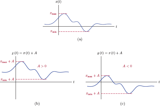
Adding an offset A to signal x(t): (a) Original signal x(t), (b)g(t) = x(t) + A with A > 0, (c)g(t) = x(t) + A with A < 0.
A signal can also be multiplied with a constant gain factor:
g(t)=Bx(t)(1.2)
The result of this operation is a signal g(t), the amplitude of which is equal to the product of the amplitude of the signal x(t) and the constant gain factor B at each time instant. This is illustrated in Fig. 1.5.
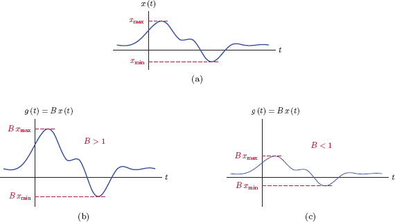
Multiplying signal x(t) with a constant gain factor: (a) Original signal x(t), (b) g(t) = Bx(t) with B > 1, (c)g(t) = Bx(t) with B < 1.
A practical example of Eqn. (1.2) is a constant-gain amplifier used for amplifying the voltage signal produced by a microphone.
Addition of two signals is accomplished by adding the amplitudes of the two signals at each time instant. For two signals x1 (t) and x2 (t), the sum
g(t)=x1(t)+x2(t)(1.3)
is computed at each time instant t = t1 by adding the values x1 (t1) and x2 (t2). This is illustrated in Fig. 1.6.
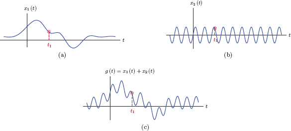
Adding continuous-time signals: (a) The signal x1 (t), (b) the signal x2 (t), (c) the sum signal g(t) = x1 (t)+x2 (t).
Signal adders are useful in a wide variety of applications. As an example, in an audio recording studio, signals coming from several microphones can be added together to create a complex piece of music.
Multiplication of two signals is carried out in a similar manner. Given two signals x1 (t) and x2(t), the product
g(t)=x1(t)x2(t)(1.4)
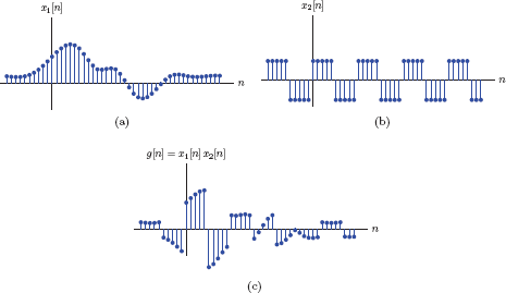
is a signal, the amplitude of which at any time instant t = t1 is equal to the product of the amplitudes of the signals x1 (t)and x2 (t) at the same time instant, that is,g(t1)= x1 (t1) x2 (t1). This is illustrated in Fig. 1.7.
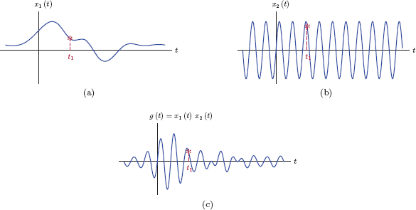
Multiplying continuous-time signals: (a) The signal x1 (t), (b) the signal x2 (t), (c) the product signal g(t) = x1 (t)x2 (t).
One example of a practical application of multiplying two signals is in modulating the amplitude of a sinusoidal carrier signal with a message signal. This will be explored when we discuss amplitude modulation in Chapter 11.
Example 1.1: Constant offset and gain
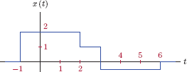
Consider the signal shown in Fig. 1.8. Sketch the signals
- g1 (t) = 1.5x(t) − 1
- g2 (t) = − 1.3x(t) + 1
Solution:
- Multiplying the signal with a constant gain factor of 1.5 causes all signal amplitudes to be scaled by 1.5. The intermediate signal g1a (t)= 1.5x(t) is shown in Fig. 1.9(a). In the next step, the signal g1 (t) = g1a (t) − 1 is obtained by lowering the graph of the the signal g1a (t) by 1 at all time instants. The result is shown in Fig. 1.9(b).
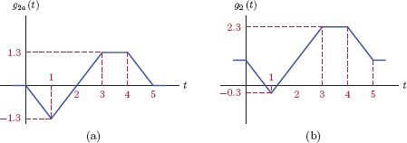
- We will proceed in a similar fashion. In this case the gain factor is negative, so the signal amplitudes will exhibit sign change. The intermediate signal g2a (t)= − 1.3x(t) is shown in Fig. 1.10(a). In the next step, the signal g2 (t)= g2a (t) + 1 is obtained by raising the graph of the the signal g2a (t) by 1 at all time instants. The result is shown in Fig. 1.10(b).

Software resources: |
See MATLAB Exercise 1.2. |
Interactive Demo: sop_demo1
The demo program “sop_demo1.m” is based on Example 1.1. It allows experimentation with elementary signal operations involving constant offset and constant gain factor. Specifically, the signal x(t) shown in Fig. 1.8 is used as the basis of the demo program, and the signal
g(t)=Bx(t)+A
is computed and graphed. The parameters A and B can be adjusted through the use of slider controls.
Software resources:
sop_demo1.m
Example 1.2: Arithmetic operations with continuous-time signals
Two signals x1 (t) and x2 (t) are shown in Fig. 1.11. Sketch the signals
- g1 (t) = x1 (t) + x2 (t)
- g2 (t) = x1 (t) x2 (t)
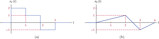
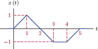
Solution: The following analytical descriptions of the signals x1 (t) and x2 (t) can be inferred from the graphical descriptions given in Fig. 1.11:
x1(t)={2,0<t<11,1<t<2-1,2<t<30,otherwiseandx2(t)={12t,0<t<2-2t+5,2<t<3t-4,3<t<40,otherwise
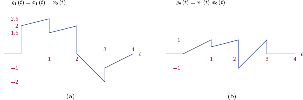
The addition of the two signals can be accomplished by adding the values in each segment separately. The analytical form of the sum is
g1(t)={12t+2,0<t<112t+1,1<t<2-2t+4,2<t<3t-4,3<t<40,otherwise(1.5)
and is shown graphically in Fig. 1.12(a).
The product of the two signals can also computed for each segment, and is obtained as
g2(t)={t,0<t<112t,1<t<22t-5,2<t<30,otherwise(1.6)
This result is shown in Fig. 1.12(b).
ex_1_2.m
Time shifting
A time shifted version of the signal x(t) can be obtained through
g(t)=x(t-td)(1.7)
where td is any positive or negative constant. Fig. 1.13 illustrates the relationship described by Eqn. (1.7). In part (a) of Fig. 1.13 the amplitude of x(t) at the time instant t = t1 is marked with a star-shaped marker. Let that marker represent a special event that takes place within the signal x(t). Substituting t = t1 + td in Eqn. (1.7) we obtain
g(t1+td)=x(t1)(1.8)
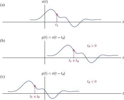
Time shifting a signal: (a) Original signal x(t), (b) time shifted signal g(t) for td > 0, (c) time shifted signal g(t) for td < 0.
Thus, in the signal g(t), the same event takes place at the time instant t = t1 + td. If td is positive, g(t) is a delayed version of x(t), and td is the amount of time delay. A negative td, on the other hand, corresponds to advancing the signal in time by an amount equal to –td.
Time scaling
A time scaled version of the signal x(t) is obtained through the relationship
g(t)=x(at)(1.9)
where a is a positive constant. Depending on the value of a, the signal g(t) is either compressed or an expanded version of x(t). Fig. 1.14 illustrates this relationship. We will use a logic similar to the one employed in explaining the time shifting behavior: In part (a) of Fig. 1.14, let the star-shaped marker at the time instant t = t1 represent a special event in the signal x(t). Substituting t = t1/a in Eqn. (1.9) we obtain
g(t1a)=x(t1)(1.10)
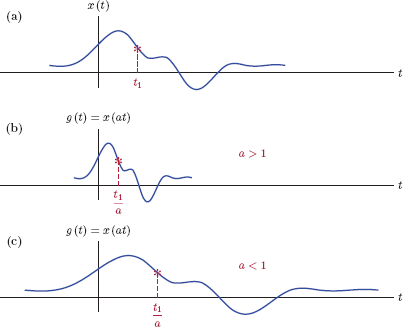
Time scaling a signal: (a) Original signal x(t), (b) time scaled signal g(t) for a > 0, (c) time scaled signal g(t) for a < 0.
The corresponding event in g(t) takes place at the time instant t = t1/a. Thus, a scaling parameter value of a > 1 results in the signal g(t) being a compressed version of x(t). Conversely, a < 1 leads to a signal g(t) that is an expanded version of x(t).
Time reversal
A time reversed version of the signal x(t) is obtained through
g(t)=x(-t)(1.11)
which is illustrated in Fig. 1.15.
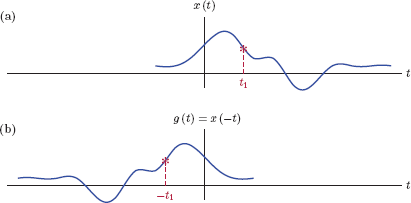
An event that takes place at the time instant t = t1 in the signal x(t) is duplicated at the time instant t = −t1 in the signal g(t). Graphically this corresponds to folding or flipping the signal around the vertical axis.
Interactive Demo: sop_demo2
The demo program “sop_demo2.m” is based on the discussion above, and allows experimentation with elementary signal operations, namely shifting, scaling and reversal of a signal as well as addition and multiplication of two signals. The desired signal operation is selected from the drop-down list control. When applicable, slider control for the time delay parameter td or the time scaling parameter a becomes available to facilitate adjustment of the corresponding value. Also, the star-shaped marker used in Figure. 1.13, Figure. 1.14, 1.15 is also shown on the graphs for x(t) and g(t) when it is relevant to the signal operation chosen.
Software resources:
sop_demo2.m
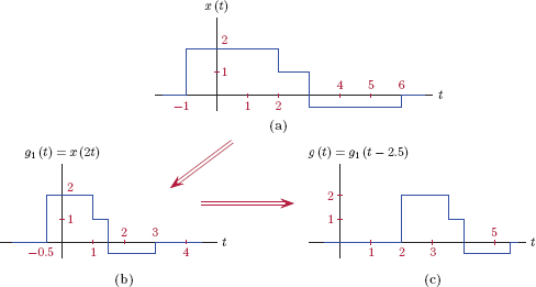
Example 1.3: Basic operations for continuous-time signals
Consider the signal x(t) shown in Fig. 1.16. Sketch the following signals:
- g(t) = x (2t − 5),
- h(t) = x(−4t + 2).
We will obtain g(t) in two steps: Let an intermediate signal be defined as g1 (t) = x (2t), a time scaled version of x(t), shown in Fig. 1.17(b). The signal g(t) can be expressed as
g(t)=g1(t-2.5)=x(2[t-2.5])=x(2t-5)
and is shown in Fig. 1.17(c).
In this case we will use two intermediate signals: Let h1 (t) = x (4t). A second intermediate signal h2 (t) can be obtained by time shifting h1 (t) so that
h2(t)=h1(t+0.5)=x(4[t+0.5])=x(4t+2)
Finally, h(t) can be obtained through time reversal of h2 (t):
h(t)=h2(-t)=x(-4t+2)
The steps involved in sketching h(t) are shown in Fig. 1.18(a)–(d).
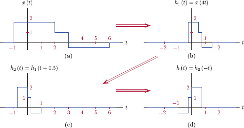
(a) The intermediate signal h1(t), (b) the intermediate signal h2(t), and (c) the signal h(t) for Example 1.3.
See MATLAB Exercise 1.3. |
Integration and differentiation
Integration and differentiation operations are used extensively in the study of linear systems. Given a continuous-time signal x(t), a new signal g(t) may be defined as its time derivative in the form
g(t)=dx(t)dt(1.12)
A practical example of this is the relationship between the current iC (t) and the voltage vC (t) of an ideal capacitor with capacitance C as given by
iC(t)=CdvC(t)dt(1.13)
For example, if the voltage in the shape of a periodic triangular waveform shown in Fig. 1.19(a) is applied to an ideal capacitor, the current that flows through the capacitor would be proportional to its derivative, resulting in a square-wave signal as shown in Fig. 1.19(b).
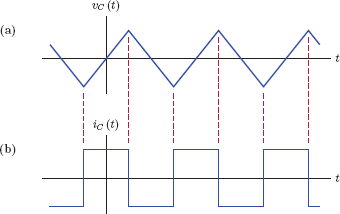
(a) A periodic triangular waveform vC (t) used as the voltage of a capacitor, and (b) the periodic square-wave current signal iC (t) that results.
Similarly, a signal can be defined as the integral of another signal in the form
g(t)=∫t-∞x(λ) dλ(1.14)
The relationship between the current iL (t) and the voltage vL (t) of an ideal inductor can serve as an example of this. Specifically we have
iL(t)=1L∫t-∞vL(λ) dλ(1.15)
If the voltage in the shape of a periodic square-wave shown in Fig. 1.20(a) is applied to an ideal inductor, the current that flows through it would be proportional to its integral, resulting in a periodic triangular waveform as shown in Fig. 1.20(b).
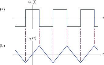
(a) A periodic square-wave signal vL (t) used as the voltage of an inductor, and (b) the periodic triangular current signal iL (t) that results.
1.3.2 Basic building blocks for continuous-time signals
There are certain basic signal forms that can be used as building blocks for describing signals with higher complexity. In this section we will study some of these signals. Mathematical models for more advanced signals can be developed by combining these basic building blocks through the use of the signal operations described in Section 1.3.1.
Unit-impulse function
We will see in the rest of this chapter as well as the chapters to follow that the unit-impulse function plays an important role in mathematical modeling and analysis of signals and linear systems. It is defined by the following equations:
δ(t)={0,if t≠0undefined,if t=0(1.16)
and
∫∞-∞δ(t) dt=1(1.17)
Note that Eqn. (1.16) by itself represents an incomplete definition of the function δ(t) since the amplitude of it is defined only when t ≠ 0, and is undefined at the time instant t = 0. Eqn. (1.17) fills this void by defining the area under the function δ(t) to be unity. The impulse function cannot be graphed using the common practice of graphing amplitude as a function of time, since the only amplitude of interest occurs at a single time instant t = 0, and it has an undefined value. Instead, we use an arrow to indicate the location of that undefined amplitude, as shown in Fig. 1.21.

In a number of problems in this text we will utilize shifted and scaled versions of impulse function. The function a δ(t − t1) represents a unit-impulse function that is time shifted by t1 and scaled by constant scale factor a. It is described through the equations
a δ(t-t1)={0,if t≠t1undefined,if t=t1(1.18)
and
∫∞-∞aδ(t-t1) dt=a(1.19)
and is shown in Fig. 1.22.
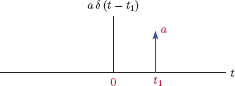
In Figs. 1.21 and 1.22 the value displayed next to the up arrow is not an amplitude value. Rather, it represents the area of the impulse function.
In Eqns. (1.17) and (1.19) the integration limits do not need to be infinite; any set of integration limits that includes the impulse would produce the same result. With any time increment Δt > 0 Eqn. (1.17) can be written in the alternative form
∫Δt-Δtδ(t)dt=1(1.20)
and Eqn. (1.19) can be written in the alternative form
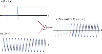
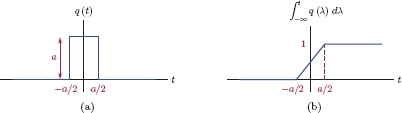
How can a function that has zero amplitude everywhere except at one point have a non-zero area under it? One way of visualizing how this might work is to start with a rectangular pulse centered at the origin, with a duration of a and an amplitude of 1/a as shown in Fig. 1.23(a). Mathematically, the pulse q(t) is defined as

Obtaining a unit impulse as the limit of a pulse with unit area. (a) The pulse q(t), (b) a narrower and taller version obtained by reducing a, (c) unit-impulse function obtained as the limit.
The area under the pulse is clearly equal to unity independent of the value of a. Now imagine the parameter a getting smaller, resulting in the pulse becoming narrower. As the pulse becomes narrower, it also becomes taller as shown in Fig. 1.23(b). The area under the pulse remains unity. In the limit, as the parameter a approaches zero, the pulse approaches an impulse, that is
This is illustrated in Fig. 1.23(c).
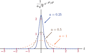
It is also possible to obtain a unit impulse as the limit of other functions besides a rectangular pulse. Another example of a function that approaches a unit impulse in the limit is the Gaussian function. Consider the limit
The Gaussian function inside the limit has unit area, and becomes narrower as the parameter a becomes smaller. This is illustrated in Fig. 1.24.
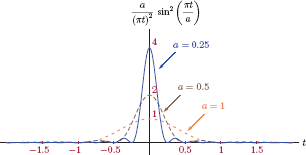
A third function that yields a unit impulse in the limit is a squared sinc pulse. It is also possible to define a unit impulse as the limit case of the squared sinc pulse:
The convergence of this limit to a unit impulse is illustrated in Fig. 1.25.
The demo program “imp_demo.m” illustrates the construction of a unit-impulse function as the limit of functions with unit area, namely a rectangular pulse, a Gaussian pulse and a squared sinc pulse. Refer to Eqns. (1.23), (1.24) and (1.25) as well as the corresponding Figs. 1.23, 1.24 and 1.25 for details.
The parameter a used in changing the shape of each of these functions can be varied by using a slider control. Observe how each function exhibits increased similarity to the unit impulse as the value of a is reduced.
Software resources:
imp_demo.m
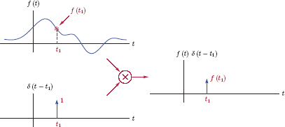
The impulse function has two fundamental properties that are useful. The first one, referred to as the sampling property1 of the impulse function, is stated as
where f(t) is any function of time that is continuous at t = t1. Intuitively, since δ (t − t1) is equal to zero for all t ≠ t1, the only value of the function f (t) that should have any significance in terms of the product f (t) δ (t − t1) is its value at t = t1. The sampling property of the unit-impulse function is illustrated in Fig. 1.26.
A consequence of Eqn. (1.26) is the sifting property of the impulse function which is expressed as
The integral of the product of a function f(t) and a time shifted unit-impulse function is equal to the value of f(t) evaluated at the location of the unit impulse. The sifting property expressed by Eqn. (1.27) is easy to justify through the use of the sampling property.
Substituting Eqn. (1.26) into Eqn. (1.27) we obtain
As discussed above, the limits of the integral in Eqn. (1.27) do not need to be infinitely large for the result to be valid; any integration interval that includes the impulse will work. Given a time increment Δt > 0, the following is also valid:
It should be clear from the foregoing discussion that the unit-impulse function is a mathematical idealization. No physical signal is capable of occurring without taking any time and still providing a non-zero result when integrated. Therefore, no physical signal that utilizes the unit-impulse function as a mathematical model can be obtained in practice. This realization naturally prompts the question “why do we need the unit-impulse signal?” or the question “how is the unit-impulse signal useful?” The answer to these questions lies in the fact that the unit-impulse function is a fundamental building block that is useful in approximating events that occur quickly. The use of the unit-impulse function allows us to look at a signal as a series of events that occur momentarily.
Consider the sifting property of the impulse function which was described by Eqn. (1.27). Through the use of the sifting property, we can focus on the behavior of a signal at one specific instant in time. By using the sifting property repeatedly at every imaginable time instant we can analyze a signal in terms of its behavior as a function of time. This idea will become clearer when we discuss impulse decomposition of a signal in the next section which will later become the basis of the development leading to the convolution operation in Chapter 2. Even though the impulse signal is not obtainable in a practical sense, it can be approximated using a number of functions; the three signals we have considered in Figs. 1.23, 1.24 and 1.25 are possible candidates when the parameter a is reasonably small.
Unit-step function
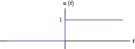
The unit-step function is useful in situations where we need to model a signal that is turned on or off at a specific time instant. It is defined as follows:
The function u(t) is illustrated in Fig. 1.27.
A time shifted version of the unit-step function can be written as
and is shown in Fig. 1.28.
Consider a sinusoidal signal given by
which oscillates for all values of t. If we need to represent a sinusoidal signal that is switched on at time t = 0, we can use the unit-step function with Eqn. (1.32), and write
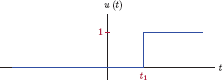
Alternatively, the signal can be switched on at an arbitrary time instant t = t1 through the use of a time shifted unit-step function:
Fig. 1.29 illustrates this use of the unit-step function for switching a signal on at a specified time instant.
This demo program illustrates the use of the unit-step function for switching a signal on at a specified time. It is based on Fig. 1.29. The delay parameter t1 for the unit-step function can be varied by using the slider control.
Software resources:
stp_demo1.m
Conversely, suppose the sinusoidal signal has been on for a long time, and we would like to turn it off at time instant t = t1. This could be accomplished by multiplication of the sinusoidal signal with a time reversed and shifted unit-step function in the form
and is illustrated in Fig. 1.30.

This demo program illustrates the use of the unit-step function for switching a signal off at a specified time. It is based on Fig. 1.30. As in “stp_demo1.m”, the delay parameter t1 for the unit-step function can be varied by using the slider control.
Software resources:
stp_demo2.m
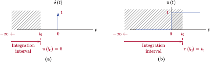
The relationship between the unit-step function and the unit-impulse function is important. The unit-step function can be expressed as a running integral of the unit-impulse function:
In Eqn. (1.33) we have changed the independent variable to λ to avoid any confusion with the upper limit t of integration. Recall that the integral of the unit-impulse function equals unity provided that the impulse is within the integration limits. This is indeed the case in Eqn. (1.33) if the upper limit of the integral is positive, that is, if t = t0 > 0. Conversely, if t = t0 < 0, then the integration interval stops short of the location of the impulse, and the result of the integral is zero. This is illustrated in Fig. 1.31.

Obtaining a unit step through the running integral of the unit impulse: (a) t = t0 < 0, (b)t = t0 > 0.
In Fig. 1.23 and Eqns. (1.22) and (1.23) we have represented the unit-impulse function as the limit of a rectangular pulse with unit area. Fig. 1.32 illustrates the running integral of such a pulse. In the limit, the result of the running integral approaches the unit-step function as a → 0.
(a) Rectangular pulse approximation to a unit impulse, (b) running integral of the rectangular pulse as an approximation to a unit step.
The unit-impulse function can be written as the derivative of the unit-step function, that is,
consistent with Eqn. (1.33).
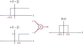
Unit-pulse function
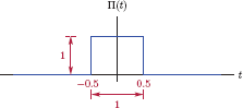
We will define the unit-pulse function as a rectangular pulse with unit width and unit amplitude, centered around the origin. Mathematically, it can be expressed as
and is shown in Fig. 1.33.
The unit-pulse function can be expressed in terms of time shifted unit-step functions as
The steps in constructing a unit-pulse signal from unit-step functions are illustrated in Fig. 1.34. It is also possible to construct a unit-pulse signal using unit-impulse functions. Let us substitute Eqn. (1.33) into Eqn. (1.36) to obtain
The result in Eqn. (1.37) can be interpreted as follows: For the result of the integral to be equal to unity, the impulse needs to appear between the integration limits. This requires that the lower limit be negative and the upper limit be positive. Thus we have
which matches the definition of the unit-pulse signal given in Eqn. (1.35). A graphical illustration of Eqn. (1.37) is given in Fig. 1.35.
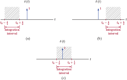
Constructing a unit pulse by integrating a unit impulse: (a) t = t0 < −1/2, (b) t = t0 > 1/2, (c) −1/2 < t < 1/2.
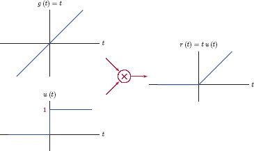
Unit-ramp function
The unit-ramp function is defined as
It has zero amplitude for t < 0, and unit slope for t ≥ 0. This behavior is illustrated in Fig. 1.36.

An equivalent definition of the unit-ramp function can be written using the product of a linear signal g(t) = t and the unit-step function as
as illustrated in Fig. 1.37.
Alternatively, the unit-ramp function may be recognized as the integral of the unit-step function:
as shown in Fig. 1.38.
We will find time shifted and time scaled versions of the unit-ramp function useful in constructing signals that have piecewise linear segments.
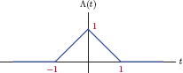
Unit-triangle function
The unit-triangle function is defined as
and is shown in Fig. 1.39.
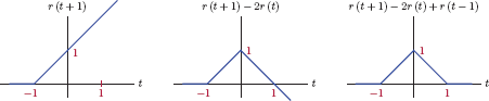
Unit-triangle function can be expressed in terms of shifted and scaled unit-ramp functions as
In order to understand Eqn. (1.43) we will observe the slope of the unit-triangle waveform in each segment. The first term r(t + 1) has a slope of 0 for t < − 1, and a slope of 1 for t > − 1. The addition of the term −2r(t) changes the slope to −1 for t > 0. The last term, r(t − 1), makes the slope 0 for t > 1. The process of constructing a unit triangle from shifted and scaled unit-ramp functions is illustrated in Fig. 1.40.
Interactive Demo: wav_demo1
The waveform explorer program “wav_demo1.m.m” allows experimentation with the basic signal building blocks discussed in Section 1.3.2. The signal x(t) that is graphed is constructed in the form
Each term xi (t), i = 1,..., 5 in Eqn. (1.44) can be a scaled and time shifted step, ramp, pulse or triangle function. Additionally, step and ramp functions can be time reversed; pulse and triangle functions can be time scaled. If fewer than five terms are needed for x(t), unneeded terms can be turned off.
Software resources:
wav_demo1.m
Sinusoidal signals
The general form of a sinusoidal signal is
where A is the amplitude of the signal, and ω0 is the radian frequency which has the unit of radians per second, abbreviated as rad/s. The parameter θ is the initial phase angle in radians. The radian frequency ω0 can be expressed as
where f0 is the frequency in Hz. This signal is shown in Fig. 1.41.
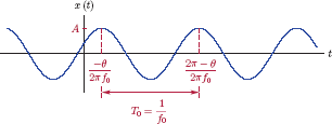
The amplitude parameter A controls the peak value of the signal. The phase θ affects the locations of the peaks:
If θ = 0, the cosine waveform has a peak at the origin t0 = 0. Other positive or negative peaks of the waveform would be at time instants that are solutions the equation
which leads to tk = k/(2f0).
With a different value of θ, the first peak is shifted to t0 = −θ/ (2πf0), the time instant that satisfies the equation 2πf0t0 + θ = 0. Other peaks of the waveform are shifted to time instants tk = (kπ − θ)/(2πf0) which are solutions to the equation
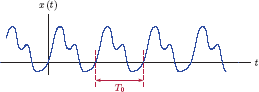
Finally, the frequency f0 controls the repetition of the waveform. Let’s refer to the part of the signal from one positive peak to the next as one cycle as shown in Fig. 1.41. When expressed in Hz, f0 is the number cycles (or periods) of the signal per second. Consequently, each cycle or period spans T0 = 1/f0 seconds.
This demo program illustrates the key properties of a sinusoidal signal based on the preceding discussion. Refer to Eqn. (1.44) and Fig. 1.41. Slider controls allow the amplitude A, the frequency f0 and the phase θ to be varied.
- Observe the value of the peak amplitude of the waveform changing in response to changes in parameter A.
- Pay attention to the reciprocal relationship between the frequency f0 and the period T0.
- Set f0 = 250 Hz, and θ = 0 degrees. Count the number of complete cycles over 40 ms in the time interval −20 ms ≤ t ≤ 20 ms. How does the number of full cycles correspond to the value of f0?
- When θ = 0, the cosine waveform has a peak at t = 0. Change the phase θ slightly in the negative direction by moving the slider control to the left, and observe the middle peak of the waveform move to the right. Observe the value of this time-delay caused by the change in θ, and relate it to Eqn. (1.47).
Software resources:
sin_demo1.m
1.3.3 Impulse decomposition for continuous-time signals
Sifting property of the unit-impulse function is given by Eqn. (1.27). Using this property, a signal x(t) can be expressed in the form
We will explore this relationship in a bit more detail to gain further insight. Suppose we wanted to approximate the signal x(t) using a series of rectangles that are each Δ wide. Let each rectangle be centered around the time instant tn = nΔ where n is the integer index, and also let the height of each rectangle be adjusted to the amplitude of the signal x(t) at the mid-point of the rectangle. Our approximation of x(t) would be in the form
which is graphically depicted in Fig. 1.42.
Let’s multiply and divide the term in the summation on the right side of Eqn. (1.49) by Δ to obtain
Furthermore, we will define pn (t) as
Clearly, pn (t) is a rectangular pulse of width Δ and height (1/Δ), and it is centered around the time instant (nΔ). It has unit area independent of the value of Δ. Substituting Eqn. (1.51) into Eqn. (1.50) leads to
We know from Eqns. (1.22) and (1.23) and Fig. 1.23 that the unit-impulse function δ(t) can be obtained as the limit of a rectangular pulse with unit area by making it narrower and taller at the same time. Therefore, the pulse pn (t) turns into an impulse if we force Δ → 0.
Thus, if we take the limit of Eqn. (1.52) as Δ → 0, the approximation becomes an equality:
In the limit2 we get pn (t) → δ (t), nΔ → λ and Δ → dλ. Also, the summation in Eqn. (1.54) turns into an integral, and we obtain Eqn. (1.48). This result will be useful as we derive the convolution relationship in the next chapter.
Interactive Demo: id_demo.m
The demo program “id_demo.m” illustrates the derivation of impulse decomposition as outlined in Eqns. (1.48) through (1.54). It shows the the progression of as defined by Eqn. (1.49) into x(t) as the value of Δ approaches zero. A slider control allows the value of Δ to be adjusted.
Software resources:
id_demo.m
1.3.4 Signal classifications
In this section we will summarize various methods and criteria for classifying the types of continuous-time signals that will be useful in our future discussions.
Real vs. complex signals
A real signal is one in which the amplitude is real-valued at all time instants. For example, if we model an electrical voltage or current with a mathematical function of time, the resulting signal x(t) is obviously real-valued. In contrast, a complex signal is one in which the signal amplitude may also have an imaginary part. A complex signal may be written in Cartesian form using its real and imaginary parts as
or in polar form using its magnitude and phase as
The two forms in Eqns. (1.55) and (1.56) can be related to each other through the following set of equations:
In deriving Eqns. (1.59) and (1.60) we have used Euler’s formula.3
Even though we will mostly focus on the use of real-valued signals in our discussion in the rest of this text, there will be times when the use of complex signal models will prove useful.
Periodic vs. non-periodic signals
A signal is said to be periodic if it satisfies
at all time instants t, and for a specific value of T0 ≠ 0. The value T0 is referred to as the period of the signal. An example of a periodic signal is shown in Fig. 1.43.
Applying the periodicity definition of Eqn. (1.61) to x(t + T0) instead of x(t) we obtain
which, when combined with Eqn. (1.61), implies that
and, through repeated use of this process, we can show that
for any integer value of k. Thus we conclude that, if a signal is periodic with period T0, then it is also periodic with periods of 2T0, 3T0,...,kT0,... where k is any integer. When we refer to the period of a periodic signal, we will imply the smallest positive value of T0 that satisfies Eqn. (1.61). In cases when we discuss multiple periods for the same signal, we will refer to T0 as the fundamental period in order to avoid ambiguity.
The fundamental frequency of a periodic signal is defined as the reciprocal of its fundamental period:
If the fundamental period T0 is expressed in seconds, then the corresponding fundamental frequency f0 is expressed in Hz.
Example 1.4: Working with a complex periodic signal
Consider a signal defined by
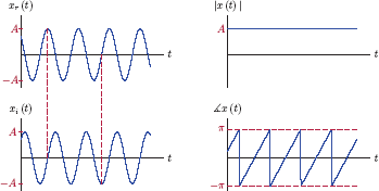
Using Eqns. (1.57) and (1.58), polar complex form of this signal can be obtained as x(t) = |x(t)| ej∠x(t), with magnitude and phase given by
and
respectively. In deriving the results in Eqns. (1.66) and (1.67) we have relied on the appropriate trigonometric identities.4 Once the magnitude |x(t)| and the phase ∡x(t) are obtained, we can express the signal x(t) in polar complex form:
The components of the Cartesian and polar complex forms of the signal are shown in Fig. 1.44. The real and imaginary parts of x(t) have a 90 degree phase difference between them. When the real part of the signal goes through a peak, the imaginary part goes through zero and vice versa. The phase of x(t) was found in Eqn. (1.66) to be a linear function of the time variable t. The broken-line appearance of the phase characteristic in Fig. 1.44 is due to normalization of the phase angles to keep them in the range −π ≤ ∡x(t) < π.
Software resources:
ex_1_4.m
Interactive Demo: cexp_demo
This demo is based on Example 1.4 and Fig. 1.44. It allows experimentation with the four graphs in Fig. 1.44 while varying the parameters A, f0, and θ. Three slider controls at the top of the graphical user interface window can be used for varying the three parameters within their prescribed ranges: 0.5 ≤ A ≤ 5, 50Hz ≤ f0 ≤ 500Hz, and −180° ≤ θ ≤ 180° respectively. Moving a slider to the right increases the value of the parameter it controls, and moving it to the left does the opposite. It is also possible to type the desired value of a parameter into the edit field associated with its slider control. Vary the parameters and observe the following:
- As the amplitude A is increased, the graphs for xr (t), xi (t) and |x(t)| scale accordingly, however, the phase ∡x(t) is not affected.
- Changing θ causes a time-delay in xr (t) and xi (t).
Software resources:
cexp_demo.m
Software resources: |
See MATLAB Exercise 1.4. |
Example 1.5: Periodicity of continuous-time sinusoidal signals
Consider two continuous-time sinusoidal signals
and
Determine the conditions under which the sum signal
is also periodic. Also, determine the fundamental period of the signal x(t) as a function of the relevant parameters of x1 (t) and x2 (t).
Solution: Based on the discussion above, we know that the individual sinusoidal signals x1 (t) and x2 (t) are periodic with fundamental periods of T1 and T2 respectively, and the following periodicity properties can be written:
where m1 and m2 are arbitrary integer values. In order for the sum signal x(t) to be periodic with period T0, we need the relationship
to be valid at all time instants. In terms of the signals x1 (t) and x2 (t) this requires
Using Eqns. (1.69) and (1.70) with Eqn. (1.72) we reach the conclusion that Eqn. (1.71) would hold if two integers m1 and m2 can be found such that
or, in terms of the frequencies involved,
The sum of two sinusoidal signals x1 (t) and x2 (t) is periodic provided that their frequencies are integer multiples of a frequency f0, i.e., f1 = m1f0 and f2 = m2f0. The period of the sum signal is T0 = 1/f0. The frequency f0 is the fundamental frequency of x(t).
The reasoning above can be easily extended to any number of sinusoidal signals added together. Consider a signal x(t) defined as
The signal x(t) is periodic provided that the frequencies of all of its components are integer multiples of a fundamental frequency f0, that is,
This conclusion will be significant when we discuss the Fourier series representation of periodic signals in Chapter 4.
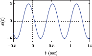
Example 1.6: More on the periodicity of sinusoidal signals
Discuss the periodicity of the signals
Solution:
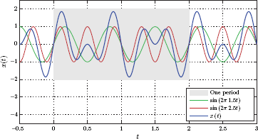
For this signal, the fundamental frequency is f0 = 0.5 Hz. The two signal frequencies can be expressed as
The resulting fundamental period is T0 = 1/f0 = 2 seconds. Within one period of x(t) there are m1 = 3 full cycles of the first sinusoid and m2 = 5 cycles of the second sinusoid. This is illustrated in Fig. 1.45.
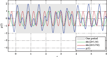
In this case the fundamental frequency is f0 = 0.25 Hz. The two signal frequencies can be expressed as
The resulting fundamental period is T0 = 1/f0 = 4 seconds. Within one period of x(t) there are m1 = 6 full cycles of the first sinusoid and m2 = 11 cycles of the second sinusoid. This is illustrated in Fig. 1.46.
ex_1_6a.m
ex_1_6b.m
Interactive Demo: sin_demo2
This demo program allows exploration of the periodicity of multi-tone signals. A signal of the type given by Eqn. (1.75) can be graphed using up to four frequencies. The beginning and the end of one period of the signal is indicated on the graph with dashed vertical lines.
Software resources:
sin_demo2.m
Deterministic vs. random signals
Deterministic signals are those that can be described completely in analytical form in the time domain. The signals that we worked with in this chapter have all been examples of deterministic signals. Random signals, on the other hand, are signals that occur due to random phenomena that cannot be modeled analytically. An example of a random signal is the speech signal converted to the form of an electrical voltage waveform by means of a microphone. A very short segment from a speech signal was shown in Fig. 1.2. Other examples of random signals are the vibration signal recorded during an earthquake by a seismograph, the noise signal generated by a resistor due to random movements and collisions of its electrons and the thermal energy those collisions produce. A common feature of these signals is the fact that the signal amplitude is not known at any given time instant, and cannot be expressed using a formula. Instead, we must try to model the statistical characteristics of the random signal rather than the signal itself. These statistical characteristics studied include average values of the signal amplitude or squared signal amplitude, distribution of various probabilities involving signal amplitude, and distribution of normalized signal energy or power among different frequencies. Study of random signals is beyond the scope of this text, and the reader is referred to one of the many excellent texts available on the subject.
1.3.5 Energy and power definitions
Energy of a signal
With physical signals and systems, the concept of energy is associated with a signal that is applied to a load. The signal source delivers the energy which must be dissipated by the load. For example, consider a voltage source with voltage v(t) connected to the terminals of a resistor with resistance R as shown in Fig. 1.47(a). Let i(t) be the current that flows through the resistor. If we wanted to use the voltage v(t) as our basis in energy calculations, the total energy dissipated in the resistor would be
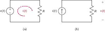
Energy dissipation in a load when (a) a voltage source is used, and (b) a current source is used.
Alternatively, consider the arrangement in Fig. 1.47(b) where a current source with a time-varying current i(t) is connected to the terminals of the same resistor. In this case, the energy dissipated in the resistor would be computed as
In the context of this text we use mathematical signal models that are independent of the physical nature of signals that are being modeled. A signal such as x(t) could represent a voltage, a current, or some other time-varying physical quantity. It would be desirable to have a definition of signal energy that is based on the mathematical model of the signal alone, without any reference to the load and to the physical quantity from which the mathematical model may have been derived. If we don’t know whether the function x(t) represents a voltage or a current, which of the two equations discussed above should we use for computing the energy produced by the signal? Comparing Eqns. (1.77) and (1.78) it is obvious that, if the resistor value is chosen to be R = 1 Ω, then both equations would produce the same numerical value:
This is precisely the approach we will take. In order to simplify our analysis, and to eliminate the need to always pay attention to the physical quantities that lead to our mathematical models, we will define the normalized energy of a real-valued signal x(t) as
provided that the integral in Eqn. (1.80) can be computed. If the signal x(t) is complex-valued, then its normalized energy is computed as
where |x(t)| is the norm of the complex signal. In situations where normalized signal energy is not computable, we may be able to compute the normalized power of the signal instead.
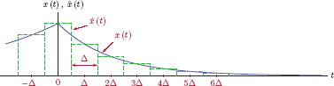
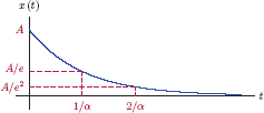
Example 1.7: Energy of a right-sided exponential signal
Compute the normalized energy of the right-sided exponential signal
where α > 0.
Solution: The signal x(t) is shown in Fig. 1.48. Notice how the signal amplitude starts with a value of x (0) = A and declines to x (1/α) = A/e after 1/α seconds elapse. At the time instant t = 2/α seconds, the amplitude is further down to x (2/α) = A/e2. Thus, the parameter α controls the rate at which the signal amplitude decays over time. The normalized energy of this signal can be computed by application of Eqn. (1.80) as
The restriction α > 0 was necessary since, without it, we could not have evaluated the integral in Eqn. (1.82).
Interactive Demo: exp_demo
This demo program is based on Example 1.7, Fig. 1.48, and Eqn. (1.82). Parameters A and α of the right-sided exponential signal x(t) can be controlled with the slider controls available.
- The shape of the right-sided exponential depends on the parameter α. Observe the key points with amplitudes A/e and A/e 2 as the parameter α is varied.
- Observe how the displayed signal energy Ex relates to the shape of the exponential signal.
Software resources:
exp_demo.m
Time averaging operator
In preparation for defining the power in a signal, we need to first define the time average of a signal. We will use the operator 〈...〉 to indicate time average. If the signal x(t) is periodic with period T0, its time average can be computed as
If the signal x(t) is non-periodic, the definition of time average in Eqn. (1.83) can be generalized with the use of the limit operator as
One way to make sense out of Eqn. (1.84) is to view the non-periodic signal x(t) as though it is periodic with an infinitely large period so that we never get to see the signal pattern repeat itself.
Example 1.8: Time average of a pulse train
Compute the time average of a periodic pulse train with an amplitude of A and a period of T0 = 1 s, defined by the equations
and
The signal x(t) is shown in Fig. 1.49.
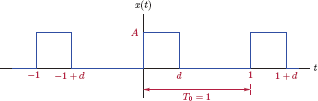
Solution: The parameter d is the width of the pulse within each period. Since the length of one period is T0 = 1 s, the parameter d can also be taken as the fraction of the period length in which the signal amplitude equals A units. In this context, d is referred to as the duty cycle of the pulse train. To compute the time average of x(t) we need to apply Eqn. (1.83) over one period:
As expected, the time average of the pulse-train signal x(t) is proportional to both the pulse amplitude A and the duty cycle d.
Interactive Demo: tavg_demo
This demo program illustrates the time averaging of pulse train x(t) as shown in Fig. 1.49 of Example 1.8 with amplitude A and duty cycle d. Values of both parameters can be adjusted using the slider controls provided. Observe how the pulse train changes when the duty cycle is varied. Also pay attention to the dashed red line that shows the value of the time average 〈x(t)〉.
Software resources:
tavg_demo.m
Power of a signal
Consider again the simple circuits in Fig. 1.47 that were used in defining normalized signal energy. Using v(t) as the voltage across the terminals of the load and i(t) as the current flowing through the load, the instantaneous power dissipated in the load resistor would be
If the load is chosen to have a value of R = 1 Ω, the normalized instantaneous power can be defined as
where x(t) could represent either the voltage or the current. Often, a more useful concept is the normalized average power defined as the time average of pnorm (t), that is
Note that this definition will work for both periodic and non-periodic signals. For a periodic signal, Eqn. (1.87) can be used with Eqn. (1.83) to yield
For a non-periodic signal, Eqn. (1.84) can be substituted into Eqn. (1.87), and we have
In our discussion, we are assuming that the signal x(t) is real-valued. If we need to consider complex-valued signals, then the definition of signal power can be generalized by using the squared norm of the signal in the time averaging operation:
Recall that the squared norm of a complex signal is computed as
where x*(t) is the complex conjugate of x(t). Thus, the power of a periodic complex signal is
and the power of a non-periodic complex signal is
Example 1.9: Power of a sinusoidal signal
Consider the signal
which is not limited in time. It is obvious that the energy of this signal can not be computed since the integral in Eqn. (1.80) would not yield a finite value. On the other hand, signal power can be computed through the use of Eqn. (1.88). The period of the signal is T0 = 1/f0, therefore
Using the appropriate trigonometric identity,5 we can write Eqn. (1.94) as
The second integral in Eqn. (1.95) evaluates to zero, since we are integrating a cosine function with the frequency 2f0 over an interval of T0 = 1/f0. The cosine function has two full cycles within this interval. Thus, the normalized average power in a sinusoidal signal with an amplitude of A is
This is a result that will be worth remembering.
Example 1.10: Right-sided exponential signal revisited
Let us consider the right-sided exponential signal of Example 1.7 again. Recall that the analytical expression for the signal was
Using Eqn. (1.89) it can easily be shown that, for α > 0, the power of the signal is Px = 0. On the other hand, it is interesting to see what happens if we allow x = 0. In this case, the signal x(t) becomes a step function:
The normalized average signal power is
and the normalized signal energy becomes infinitely large, i.e., Ex → ∞.
Energy signals vs. power signals
In Examples 1.7 through 1.10 we have observed that the concept of signal energy is useful for some signals and not for others. Same can be said for signal power. Based on our observations, we can classify signals encountered in practice into two categories:
- Energy signals are those that have finite energy and zero power, i.e., Ex < ∞, and Px = 0.
- Power signals are those that have finite power and infinite energy, i.e., Ex → ∞, and Px < ∞.
Just as a side note, all voltage and current signals that can be generated in the laboratory or that occur in the electronic devices that we use in our daily lives are energy signals. A power signal is impossible to produce in any practical setting since doing so would require an infinite amount of energy. The concept of a power signal exists as a mathematical idealization only.
RMS value of a signal
The root-mean-square (RMS) value of a signal x(t) is defined as
The time average in Eqn. (1.97) is computed through the use of either Eqn. (1.83) or Eqn. (1.84), depending on whether x(t) is periodic or not.
Example 1.11: RMS value of a sinusoidal signal
In Example 1.9, we have found the normalized average power of the sinusoidal signal x(t) = A sin (2πf0t + θ) to be Px = 〈x2(t)〉 = A2/2. Based on Eqn. (1.97), the RMS value of this signal is
as illustrated in Fig. 1.50.

Example 1.12: RMS value of a multi-tone signal
Consider the two-tone signal given by
where the two frequencies are distinct, i.e., f1 ≠ f2. Determine the RMS value and the normalized average power of this signal.
Solution: Computation of both the RMS value and the normalized average power for the signal x(t) requires the computation of the time average of x2 (t). The square of the signal x(t) is
Using the trigonometric identities6 Eqn. (1.99) can be written as
We can now apply the time averaging operator to x 2 (t) to yield
The time average of each of the cosine terms in Eqn. (1.100) is equal to zero, and we obtain
Thus, the RMS value of the signal x(t) is
and its normalized average power is
The generalization of these results to signals containing more than two sinusoidal components is straightforward. If x(t) contains M sinusoidal components with amplitudes a1,a2,...,aM, and distinct frequencies f1,f2,...,fM, its RMS value and normalized average power are
and
respectively.
1.3.6 Symmetry properties
Some signals have certain symmetry properties that could be utilized in a variety of ways in the analysis. More importantly, a signal that may not have any symmetry properties can still be written as a linear combination of signals with certain symmetry properties.
Even and odd symmetry
A real-valued signal is said to have even symmetry if it has the property
for all values of t. A signal with even symmetry remains unchanged when it is time reversed. Fig. 1.51(a) shows an example of a signal with even symmetry property. Similarly, a real-valued signal is said to have odd symmetry if it has the property
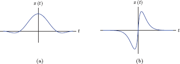
for all t. Time reversal has the same effect as negation on a signal with odd symmetry. This is illustrated in Fig. 1.51(b).
As a specific example the signal x(t) = cos(ωt) has even symmetry since cos (−ωt) = cos (ωt). Similarly, the signal x(t) = sin(ωt) has odd symmetry since sin (−ωt) = − sin (ωt).
Decomposition into even and odd components
It is always possible to split a real-valued signal into two components in such a way that one of the components is an even function of time, and the other is an odd function of time. Consider the following representation of the signal x(t):
where the two components xe (t) and xo (t) are defined as
and
The definitions of the two signals xe (t) and xo (t) guarantee that they always add up to x(t). Furthermore, symmetry properties xe(−t) = xe (t) and xo(−t) = −xo (t) are guaranteed by the definitions of the signals xe (t) and xo (t) regardless of any symmetry properties the signal x(t) may or may not possess. Symmetry properties of xe (t) and xo (t) can be easily verified by forming the expressions for xe (−t) and xo (−t) and comparing them to Eqns. (1.109) and (1.110).
We will refer to xe (t) and xo (t) as the even component and the odd component of x(t) respectively.
Example 1.13: Even and odd components of a rectangular pulse
Determine the even and the odd components of the rectangular pulse signal
which is shown in Fig. 1.52.
Solution: The even component of the signal x(t) as computed from Eqn. (1.109) is
Its odd component is computed using Eqn. (1.110) as
The two components of x(t) are graphed in Fig. 1.53.
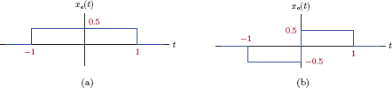
(a) The even component, and (b) the odd component of the rectangular pulse signal of Example 1.13.
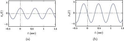
Example 1.14: Even and odd components of a sinusoidal signal
Consider the sinusoidal signal
What symmetry properties does this signal have, if any? Determine its even and odd components.
Solution: The signal x(t) is shown in Fig. 1.54. It can be observed that it has neither even symmetry nor odd symmetry.
We will use Eqns. (1.109) and (1.110) in decomposing this signal into its even and odd components. The even component is
Using the appropriate trigonometric identity,7 Eqn. (1.114) can be written as
Similarly, the odd component of x(t) is
which, through the use of the same trigonometric identity, can be written as
Even and odd components of x(t) are shown in Fig. 1.55.
ex_1_14.m
Symmetry properties for complex signals
Even and odd symmetry definitions given by Eqns. (1.106) and (1.107) for real-valued signals can be extended to work with complex-valued signals as well. A complex-valued signal is said to be conjugate symmetric if it satisfies
for all t. For a signal with conjugate symmetry, time reversal has the same effect as complex conjugation. Similarly, a complex-valued signal is said to be conjugate antisymmetric if it satisfies
for all t. If a signal is conjugate antisymmetric, time reversing it causes the signal to be conjugated and negated simultaneously.
It is easy to see from Eqns. (1.116) and (1.106) that, if the signal is real-valued, that is, if x(t) = x*(t), the definition of conjugate symmetry reduces to that of even symmetry. Similarly, conjugate antisymmetry property reduces to odd symmetry for a real valued x(t) as revealed by a comparison of Eqns. (1.117) and (1.107).
Example 1.15: Symmetry of a complex exponential signal
Consider the complex exponential signal
What symmetry property does this signal have, if any?
Solution: Time reversal of x(t) results in
Complex conjugate of the signal x(t) is
Since x(−t) = x*(t), we conclude that the signal x(t) is conjugate symmetric.
Decomposition of complex signals
It is possible to express any complex signal x(t) as the sum of two signals
such that xE (t) is conjugate symmetric, and xO (t) is conjugate antisymmetric. The two components of the decomposition in Eqn. (1.121) are computed as
and
Definitions of xE (t) and xO (t) ensure that they always add up to x(t). Furthermore, the two components are guaranteed to have the conjugate symmetry and conjugate antisymmetry properties respectively.
By conjugating the first component xE (t) we get
proving that xE (t) is conjugate symmetric. Conjugation of the other component xO (t) yields
proving that xO (t) is conjugate antisymmetric.
1.3.7 Graphical representation of sinusoidal signals using phasors
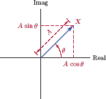
In certain situations we find it convenient to represent a sinusoidal signal with a complex quantity referred to as a phasor. Use of the phasor concept is beneficial in analyzing linear systems in which multiple sinusoidal signals may exist with the same frequency but with differing amplitude and phase values. Consider again a sinusoidal signal in the form
with three adjustable parameters, namely the amplitude A, the phase θ, and the frequency f0. Using Euler’s formula,8 it is possible to express the sinusoidal signal in Eqn. (1.124) as the real part of a complex signal in the form
The exponential function in Eqn. (1.125) can be factored into two terms, yielding
Let the complex variable X be defined as
The complex variable X can be viewed as a vector with norm A and angle θ. Vector interpretation of X is illustrated in Fig. 1.56.
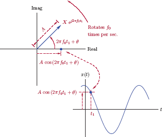
Using X in Eqn. (1.126), we obtain
In Eqn. (1.128) the exponential term ej2πf0t represents rotation. It is also complex-valued, and has unit norm. Its angle 2πf0t is a linear function of time. Over an interval of one second, the angle of the exponential term grows by 2πf0 radians, corresponding to f0 revolutions around the origin. The expression in brackets in Eqn. (1.128) combines the vector X with this exponential term. The combination represents a vector with norm A and initial phase angle θ that rotates at the rate of f0 revolutions per second. We will refer to this rotating vector as a phasor. At any time instant, the amplitude of the signal x(t) equals the real part of the phasor. This relationship is illustrated in Fig. 1.57.
Interactive Demo: phs_demo
The demo program in “phs demo.m” provides a graphical user interface for experimenting with phasors.
The graph window in the upper right section depicts the complex plane. One or two phasors can be visible; the first phasor is shown in blue, and the second phasor is shown in red. The real part of each phasor is shown with thick dashed lines of the same color as the phasor.
The graph window at the bottom shows the time-domain representation of the signal that corresponds to each phasor, using the same color scheme. The sum of the two sinusoidal signals is shown in black. The real part of each phasor, displayed with thick dashed lines on the complex plane, is duplicated on the time graph to show its relationship to the respective time-varying signal.
The norm, phase angle and rotation rate of each phasor can be specified by entering the values of the parameters into fields marked with the corresponding color, blue or red. The program accepts rotation frequencies in the range 0.1 ≤ f ≤ 10 Hz. Magnitude values can be from 0.5 to 3. Initial phase angles must naturally be in the range − 180 ≤ θ ≤ 180 degrees.
Visibility of a phasor and its associated signals can be turned on and off using the checkbox controls next to the graph window. The time variable can be advanced by clicking on the arrow button next to the slider control. As t is increased, each phasor rotates counterclockwise at its specified frequency.
Software resources:
phs_demo.m
Software resources: |
See MATLAB Exercise 1.5. |
1.4 Discrete-Time Signals
Discrete-time signals are not defined at all time instants. Instead, they are defined only at time instants that are integer multiples of a fixed time increment T, that is, at t = nT. Consequently, the mathematical model for a discrete-time signal is a function x [n] in which independent variable n is an integer, and is referred to as the sample index. The resulting signal is an indexed sequence of numbers, each of which is referred to as a sample of the signal. Discrete-time signals are often illustrated graphically using stem plots, an example of which is shown in Fig. 1.58.

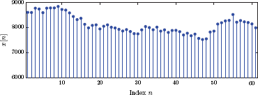
As a practical example of a discrete-time signal, daily closing values of the Dow Jones Industrial Average for the first three months of 2003 are shown in Fig. 1.59. In this case the time interval T corresponds to a day, and signal samples are indexed with integers corresponding to subsequent days of trading.
Sometimes discrete-time signals are also modeled using mathematical functions. For example
is a discrete-time sinusoidal signal. In some cases it may be more convenient to express a signal in a tabular form. A compact way of tabulating a signal is by listing the significant signal samples between a pair of braces, and separating them with commas:
The up-arrow indicates the position of the sample index n = 0, so we have x [−1] = 3.7, x[0] = 1.3, x [1] = −1.5, x [2] = 3.4, and x [3] = 5.9.
If the significant range of signal samples to be tabulated does not include n = 0, then we specify which index the up-arrow indicates. For example
indicates that x [4] = 1.1, x [5] = 2.5, x [6] = 3.7, x [7] = 3.2, and x [8] = 2.6.
For consistency in handling discrete-time signals we will assume that any discrete-time signal x [n] has an infinite number of samples for −∞ < n < ∞. If a signal is described in tabular form as shown in Eqns. (1.129) and (1.130), any samples not listed will be taken to have zero amplitudes.
In a discrete-time signal the time variable is discrete, yet the amplitude of each sample is continuous. Even if the range of amplitude values may be limited, any amplitude within the prescribed range is allowed.
If, in addition to limiting the time variable to the set of integers, we also limit the amplitude values to a discrete set, the resulting signal is called a digital signal. In the simplest case there are only two possible values for the amplitude of each sample, typically indicated by “0” and “1”. The corresponding signal is called a binary signal. Each sample of a binary signal is called a bit which stands for binary digit. Alternatively each sample of a digital signal could take on a value from a set of M allowed values, and the resulting digital signal is called an M -ary signal.
Software resources: |
See MATLAB Exercise 1.6. |
1.4.1 Signal operations
Basic signal operations for continuous-time signals were discussed in Section 1.3.1. In this section we will discuss corresponding signal operations for discrete-time signals. Arithmetic operations for discrete-time signals bear strong resemblance to their continuous-time counterparts. Discrete-time versions of time shifting, time scaling and time reversal operations will also be discussed. Technically the use of the word “time” is somewhat inaccurate for these operations since the independent variable for discrete-time signals is the sample index n which may or may not correspond to time. We will, however, use the established terms of time shifting, time scaling and time reversal while keeping in mind the distinction between t and n. More advanced signal operations such as convolution will be covered in later chapters.
Arithmetic operations
Consider a discrete-time signal x[n]. A constant offset value can be added to this signal to obtain
The offset A is added to each sample of the signal x[n]. If we were to write Eqn. (1.131) for specific values of the index n we would obtain
and so on. This is illustrated in Fig. 1.60.
![Figure showing Adding an offset A to signal x[n]: (a) Original signal x[n], (b) g[n] = x[n] + A with A > 0, (c) g[n] = x[n] + A with A < 0.](http://imgdetail.ebookreading.net/data/1/9781466598546/9781466598546__signals-and-systems__9781466598546__image__051x001.png)
Adding an offset A to signal x[n]: (a) Original signal x[n], (b) g[n] = x[n] + A with A > 0, (c) g[n] = x[n] + A with A < 0.
Multiplication of the signal x [n] with gain factor B is expressed in the form
The value of each sample of the signal g [n] is equal to the product of the corresponding sample of x[n] and the constant gain factor B. For individual index values we have
and so on. This is illustrated in Fig. 1.61.
![Figure showing Multiplying signal x[n] with a constant gain factor B: (a) Original signal x[n], (b) g[n] = Bx[n] with B > 1, (c) g[n] = Bx[n] with B < 1.](http://imgdetail.ebookreading.net/data/1/9781466598546/9781466598546__signals-and-systems__9781466598546__image__052x001.png)
Multiplying signal x[n] with a constant gain factor B: (a) Original signal x[n], (b) g[n] = Bx[n] with B > 1, (c) g[n] = Bx[n] with B < 1.
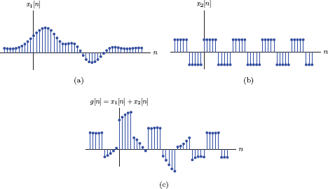
Addition of two discrete-time signals is accomplished by adding the amplitudes of the corresponding samples of the two signals. Let x1[n] and x2[n] be the two signals being added. The sum
is computed for each value of the index n as
This is illustrated in Fig. 1.62.
Two discrete-time signals can also be multiplied in a similar manner. The product of two signals x1[n] and x2[n] is
which can be written for specific values of the index as
and is shown in Fig. 1.63.
Time shifting
Since discrete-time signals are defined only for integer values of the sample index, time shifting operations must utilize integer shift parameters. A time shifted version of the signal x[n] is obtained as
where k is any positive or negative integer. The relationship between x[n] and g[n] is illustrated in Fig. 1.64.
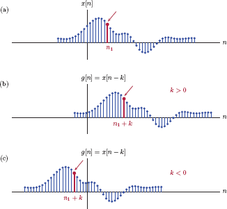
In part (a) of Fig. 1.64 the sample of x[n] at index n1 is marked with a thicker stem. Let that sample correspond to a special event in signal x[n]. Substituting n = n1 + k in Eqn. (1.135) we have
It is clear from Eqn. (1.136) that the event that takes place in x[n] at index n = n1 takes place in g[n] at index n = n1 + k.If k is positive, this corresponds to a delay by k samples. Conversely, a negative k implies an advance.
Time scaling
For discrete-time signals we will consider time scaling in the following two forms:
and
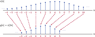
Let us first consider the form in Eqn. (1.137). The relationship between x[n] and g[n] = x[kn] is illustrated in Fig. 1.65 for k = 2 and k = 3.
![Figure showing Time scaling a signal x[n] to obtain g[n] = x[kn]: (a) Original signal x[n], (b) g[n] = x[2n], (c) g[n] = x[3n].](http://imgdetail.ebookreading.net/data/1/9781466598546/9781466598546__signals-and-systems__9781466598546__image__055x001.png)
Time scaling a signal x[n] to obtain g[n] = x[kn]: (a) Original signal x[n], (b) g[n] = x[2n], (c) g[n] = x[3n].
It will be interesting to write this relationship for several values of the index n. For k = 2 we have
which suggests that g[n] retains every other sample of x[n], and discards the samples between them. This relationship is further illustrated in Fig. 1.66.
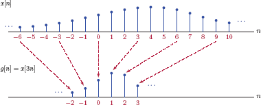
For k = 3, samples of g[n] are
In this case every third sample of x[n] is retained, and the samples between them are discarded, as shown in Fig. 1.67.
This raises an interesting question: Does the act of discarding samples lead to a loss of information, or were those samples redundant in the first place? The answer depends on the characteristics of the signal x[n], and will be explored when we discuss downsampling and decimation in Chapter 6.
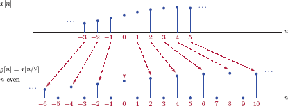
An alternative form of time scaling for a discrete-time signal was given by Eqn. (1.138). Consider for example, the signal g[n] defined based on Eqn. (1.138) with k = 2:
Since the index of the signal on the right side of the equal sign is n/2, the relationship between g[n] and x[n] is defined only for values of n that make n/2 an integer. We can write
The sample amplitudes of the signal g[n] for odd values of n are not linked to the signal x[n] in any way. For the sake of discussion let us set those undefined sample amplitudes equal to zero. Thus, we can write a complete description of the signal g[n]
Fig. 1.68 illustrates the process of obtaining g[n] from x[n] based on Eqn. (1.140). The relationship between x[n]and g[n]is known as upsampling, and will be discussed in more detail in Chapter 6 in the context of interpolation.
Time reversal
A time reversed version of the signal x[n] is
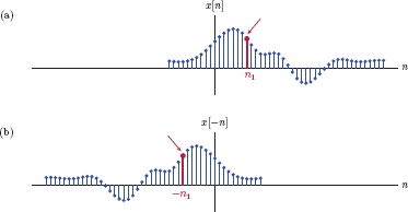
An event that takes place at index value n = n1 in the signal x[n] takes place at index value n = −n1 in the signal g[n]. Graphically this corresponds to folding or flipping the signal x[n] around n = 0 axis as illustrated in Fig. 1.69.
1.4.2 Basic building blocks for discrete-time signals
In this section we will look at basic discrete-time signal building blocks that are used in constructing mathematical models for discrete-time signals with higher complexity. We will see that many of the continuous-time signal building blocks discussed in Section 1.3.2 have discrete-time counterparts that are defined similarly, and that have similar properties. There are also some fundamental differences between continuous-time and discrete-time versions of the basic signals, and these will be indicated throughout our discussion.
Unit-impulse function
The discrete-time unit-impulse function is defined by
and is shown graphically in Fig. 1.70.
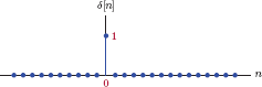
As is evident from the definition in Eqn. (1.142) and Fig. 1.70, the discrete-time unit-impulse function does not have the complications associated with its continuous-time counterpart. The signal δ [n] is unambiguously defined for all integer values of the sample index n.
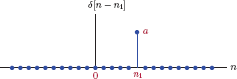
Shifted and scaled versions of the discrete-time unit-impulse function are used often in problems involving signal-system interaction. A unit-impulse function that is scaled by a and time shifted by n1 samples is described by
and is shown in Fig. 1.71.
The fundamental properties of the continuous-time unit-impulse function discussed in Section 1.3.2 can be readily adapted to its discrete-time counterpart. The sampling property of the discrete-time unit-impulse function is expressed as
It is important to interpret Eqn. (1.144) correctly: x[n] and δ[n − n1] are both infinitely long discrete-time signals, and can be graphed in terms of the sample index n as shown in Fig. 1.72.
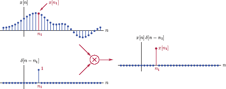
The claim in Eqn. (1.144) is easy to justify: If the two signals x[n] and δ[n − n1]are multiplied on a sample-by-sample basis, the product signal is equal to zero for all but one value of the sample index n, and the only non-zero amplitude occurs for n = n1. Mathematically we have
which is equivalent to the right side of Eqn. (1.144).
The sifting property for the discrete-time unit-impulse function is expressed as
which easily follows from Eqn. (1.144). Substituting Eqn. (1.144) into Eqn. (1.146) we obtain
where we have relied on the sum of all samples of the impulse signal being equal to unity. The result of the summation in Eqn. (1.146) is a scalar, the value of which equals sample n1 of the signal x[n].
Unit-step function
The discrete-time unit-step function can also be defined in a way similar to its continuous-time version:
The function u[n] is shown in Fig. 1.73.
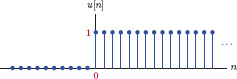
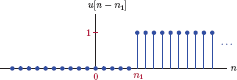
As in the case of the discrete-time unit-impulse function, this function also enjoys a clean definition without any of the complications associated with its continuous-time counterpart. Eqn. (1.148) provides a complete definition of the discrete-time unit-step function for all integer values of the sample index n. A time shifted version of the discrete-time unit-step function can be written as
and is illustrated in Fig. 1.74.
Recall that a continuous-time unit-impulse could be obtained as the first derivative of the continuous-time unit-step. An analogous relationship exists between the discrete-time counterparts of these signals. It is possible to express a discrete-time unit-impulse signal as the first difference of the discrete-time unit-step signal:
This relationship is illustrated in Fig. 1.75.

Obtaining a discrete-time unit-impulse from a discrete-time unit-step through first difference.
Conversely, a unit-step signal can be constructed from unit-impulse signals through a running sum in the form
This is analogous to the running integral relationship between the continuous-time versions of these signals, given by Eqn. (1.33). In Eqn. (1.151) we are adding the samples of a unit-step signal δ[k] starting from k = −∞ up to and including the sample for k = n. If n, the upper limit of the summation, is zero or positive, the summation includes the only sample with unit amplitude, and the result is equal to unity. If n < 0, the summation ends before we reach that sample, and the result is zero. This is shown in Fig. 1.76.
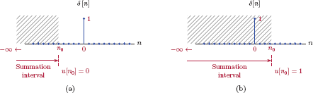
Obtaining a discrete-time unit-step from a discrete-time unit-impulse through a running sum: (a) n = n0 < 0, (b) n = n0 > 0.
An alternative approach for obtaining a unit-step from a unit-impulse is to use
in which we add the signals δ[n],δ[n−1],δ[n−2],...,δ[n−k] to construct a unit-step signal. This is an example of impulse decomposition that will be discussed in Section 1.4.3.
Unit-ramp function
The discrete-time version of the unit-ramp function is defined as
and is shown in Fig. 1.77.
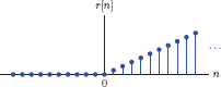
The definition in Eqn. (1.153) can be written in a more compact form as the product of the linear signal g[n] = n and the unit-step function. We can write r[n]as
which is illustrated in Fig. 1.78.

Alternatively, the discrete-time unit-ramp function can be expressed as a running summation applied to the discrete-time unit-step function in the form
By trying out the summation in Eqn. (1.155) for a few different values of the index n it is easy to see that it produces values consistent with the definition of the unit-ramp function given by Eqn. (1.154). This is analogous to the relationship between the continuous-time versions of these signals where a running integral is used for obtaining a continuous-time unit-ramp from a continuous-time unit-step as stated in Eqn. (1.41). The process of obtaining a discrete-time unit-ramp through a running sum is illustrated in Fig. 1.79.
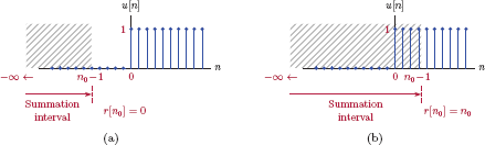
Obtaining a discrete-time unit-ramp from a discrete-time unit-step through a running sum: (a) n = n0 < 0, (b) n = n0 > 0.
Sinusoidal signals
A discrete-time sinusoidal signal is in the general form
where A is the amplitude, Ω0 is the angular frequency in radians, and θ is the phase angle which is also in radians. The angular frequency Ω0 can be expressed as
The parameter F0, a dimensionless quantity, is referred to as the normalized frequency of the sinusoidal signal. Fig. 1.80 illustrates discrete-time sinusoidal signals for various values of Ω0.
![Figure showing Discrete-time sinusoidal signal x[n] = 3 cos(Ω0n + Ω/10) for (a) Ω0 = 0.05 rad, (b) Ω0 = 0.1 rad, (c) Ω0 = 0.2 rad.](http://imgdetail.ebookreading.net/data/1/9781466598546/9781466598546__signals-and-systems__9781466598546__image__063x001.png)
Discrete-time sinusoidal signal x[n] = 3 cos(Ω0n + Ω/10) for (a) Ω0 = 0.05 rad, (b) Ω0 = 0.1 rad, (c) Ω0 = 0.2 rad.
At this point we will note a fundamental difference between a discrete-time sinusoidal signal and its continuous-time counterpart:
- A continuous-time sinusoidal signal was defined by Eqn. (1.44). Its parameter ω0 is in rad/s since it appears next to the time variable t, and the product ω0t must be in radians to qualify as the argument of a trigonometric function.
- In contrast, the parameter Ω0 is in radians since it appears next to a dimensionless index parameter n, and the product Ω0n must be in radians. For this reason, Ω0 is referred to as the angular frequency of the discrete-time sinusoidal signal.
Even though the word “frequency” is used, Ω0 is not really a frequency in the traditional sense, but rather an angle. In support of this assertion, we will see in later parts of this text that values of Ω0 outside the range −π ≤ Ω0 < π are mathematically indistinguishable from values within that range.
Similar reasoning applies to the parameter F0: It is not really a frequency but a dimensionless quantity that can best be thought of as a “percentage”. In order to elaborate further on the meanings of the parameters Ω0 and F0, we will consider the case of obtaining a discrete-time sinusoidal signal from a continuous-time sinusoidal signal in the form
Let us evaluate the amplitude of xa (t) at time instants that are integer multiples of Ts, and construct a discrete-time signal with the results.
This is illustrated in Fig. 1.81.
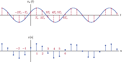
Since the signal xa (t) is evaluated at intervals of Ts, the number of samples taken per unit time is
Substituting Eqn. (1.160) into Eqn. (1.159) we obtain
which reveals the meaning of the normalized frequency F0:
The act of constructing a discrete-time signal by evaluating a continuous-time signal at uniform intervals is called sampling, and will be discussed in more detail in Chapter 6. The parameters fs and Ts are referred to as the sampling rate and the sampling interval respectively. Eqn. (1.162) suggests that the normalized frequency F0 is essentially the frequency f0 of the continuous-time sinusoid expressed as a percentage of the sampling rate.
1.4.3 Impulse decomposition for discrete-time signals
Consider an arbitrary discrete-time signal x[n]. Let us define a new signal xk[n] by using the k-th sample of the signal x[n] in conjunction with a time shifted unit-impulse function as
The signal xk[n] is a scaled and time shifted impulse signal, the only non-trivial sample of which occurs at index n = k with an amplitude of x [k]. If we were to repeat Eqn. (1.163) for all possible values of k, we would obtain an infinite number of signals xk[n] for k = −∞,...,∞. In each of these signals there would only be one non-trivial sample the amplitude of which equals the amplitude of the corresponding sample of x[n]. For example, consider the signal
The signals xk[n] for this case would be as follows:
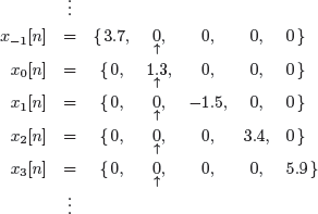
The signal x[n] can be reconstructed by adding these components together.
Eqn. (1.164) represents an impulse decomposition of the discrete-time signal x[n]. We will use it to derive the convolution relationship in Chapter 3.
1.4.4 Signal classifications
Discussion in this section will parallel that of Section 1.3.4 for continuous-time signals.
Real vs. complex signals
A discrete-time signal may be real or complex valued. A complex signal can be written in Cartesian form using its real and imaginary parts as
or in polar form using its magnitude and phase as
The equations to convert from one complex form to the other are identical to those for continuous-time complex signals.
Periodic vs. non-periodic signals
A discrete-time signal is said to be periodic if it satisfies
for all values of the integer index n and for a specific value of N ≠ 0. The parameter N is referred to as the period of the signal. An example of a periodic discrete-time signal is shown in Fig. 1.82.
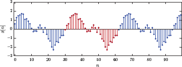
A discrete-time signal that is periodic with a period of N samples is also periodic with periods of 2N, 3N,..., kN for any positive integer k. Applying the periodicity definition of Eqn. (1.167) to x[n + N] instead of x[n] yields
Substituting Eqn. (1.168) into Eqn. (1.167) we obtain
and, through repeated use of this process, we can show that
The smallest positive value of N that satisfies Eqn. (1.167) is called the fundamental period. To avoid ambiguity when we refer to the period of a signal, fundamental period will be implied unless we specifically state otherwise. The normalized fundamental frequency of a discrete-time periodic signal is the reciprocal of its fundamental period, i.e.,
Periodicity of discrete-time sinusoidal signals
The general form of a discrete-time sinusoidal signal x[n] was given by Eqn. (1.161). For x[n] to be periodic, it needs to satisfy the periodicity condition given by Eqn. (1.167). Specifically we need
For Eqn. (1.172) to hold, the arguments of the cosine functions must differ by an integer multiple of 2π. This requirement results in
and consequently
for the period N. Since we are dealing with a discrete-time signal, there is the added requirement that the period N obtained from Eqn. (1.174) must be an integer value. Thus, the discrete-time sinusoidal signal defined by Eqn. (1.161) is periodic provided that Eqn. (1.174) yields an integer value for N. The fundamental period of the sinusoidal signal is then obtained by using the smallest integer value of k, if any, that results in N being an integer.
It should be obvious from the foregoing discussion that, contrary to a continuous-time sinusoidal signal always being periodic, a discrete-time sinusoidal signal may or may not be periodic. The signal will not be periodic, for example, if the normalized frequency F0 is an irrational number so that no value of k produces an integer N in Eqn. (1.174).
Example 1.16: Periodicity of a discrete-time sinusoidal signal
Check the periodicity of the following discrete-time signals:
- x[n] = cos(0.2n)
- x[n] = cos(0.2πn + π/ 5)
- x[n] = cos(0.3πn − π/10)
Solution:
The angular frequency of this signal is Ω0 = 0.2 radians which corresponds to a normalized frequency of
This results in a period
Since no value of k would produce an integer value for N, the signal is not periodic.
In this case the angular frequency is Ω0 = 0.2π radians, and the normalized frequency is F0 = 0.1. The period is
For k = 1 we have N = 10 samples as the fundamental period. The signal x[n]is shown in Fig. 1.83.
For this signal the angular frequency is Ω0 = 0.3π radians, and the corresponding normalized frequency is F0 = 0.15. The period is
The smallest positive integer k that would result in an integer value for the period N is k = 3. Therefore, the fundamental period is N = 3/0.15 = 20 samples. The signal x[n] is shown in Fig. 1.84.
It is interesting to observe from Fig. 1.84 that the period of N = 20 samples corresponds to three full cycles of the continuous-time sinusoidal signal from which x[n] may have been derived (see the outline shown in the figure). This is due to the fact that k = 3 and, based on Eqn. (1.173), the argument of the cosine function is advanced by
after one period of 20 samples.
![Figure showing the signal x[n] for part (b) of Example 1.16.](http://imgdetail.ebookreading.net/data/1/9781466598546/9781466598546__signals-and-systems__9781466598546__image__068x001.png)
![Figure showing the signal x[n] for part (c) of Example 1.16.](http://imgdetail.ebookreading.net/data/1/9781466598546/9781466598546__signals-and-systems__9781466598546__image__068x002.png)
Software resources:
ex_1_16a.m
ex_1_16b.m
ex_1_16c.m
Example 1.17: Periodicity of a multi-tone discrete-time sinusoidal signal
Comment on the periodicity of the two-tone discrete-time signal
Solution: The signal is in the form
with
and
Corresponding normalized frequencies are F1 = 0.2 and F2 =0.24. The period of each component can be found as follows:
Thus the fundamental period for x1[n] is N1 = 5 samples, and the fundamental period for x2[n] is N2 = 25 samples. The period of the total signal x[n] is N = 25 samples. Within the period of N = 25 samples, the first component x1[n] completes 5 cycles since N =5N1. The second component completes 6 cycles since k2 = 6 to get an integer value for N2.This is illustrated in Fig. 1.85.
![Figure showing the signals used in Example 1.17: (a) x1[n], (b) x2[n], (c) x[n] = x1[n] + x2[n].](http://imgdetail.ebookreading.net/data/1/9781466598546/9781466598546__signals-and-systems__9781466598546__image__069x001.png)
Software resources:
ex_1_17.m
Deterministic vs. random signals
Deterministic signals are signals that can be described completely in analytical form in the time domain. Random signals are signals that cannot be modeled analytically. They can be analyzed in terms of their statistical properties. Study of random signals is beyond the scope of this text, and the reader is referred to one of the many excellent texts available on the subject.
1.4.5 Energy and power definitions
Energy of a signal
The energy of a real-valued discrete-time signal is computed as
provided that it can be computed. If the signal under consideration is complex-valued, its energy is given by
Time averaging operator
We will use the operator 〈...〉 to indicate time average. If the signal x[n] is periodic with period N, its time average can be computed as
For a signal x[n] that is non-periodic, the definition of time average in Eqn. (1.181) can be generalized with the use of the limit operator as
Power of a signal
The average power of a real-valued discrete-time signal is computed as
This definition works for both periodic and non-periodic signals. For a periodic signal, Eqn. (1.181) can be used with Eqn. (1.183) to yield
For a non-periodic signal, Eqn. (1.182) can be substituted into Eqn. (1.183) to yield
Eqns. (1.184) and (1.185) apply to signals that are real-valued. If the signal under consideration is complex, then Eqns. (1.184) and (1.185) can be generalized by using the squared norm of the signal x[n], i.e.,
Thus, the power of a periodic complex signal is
and the power of a non-periodic complex signal is
Energy signals vs. power signals
As with continuous-time signals, it is also possible to classify discrete-time signals based on their energy and power:
- Energy signals are those that have finite energy and zero power, i.e., Ex < ∞, and Px = 0.
- Power signals are those that have finite power and infinite energy, i.e., Ex → ∞, and Px < ∞.
1.4.6 Symmetry properties
Definitions of the symmetry properties given in Section 1.3.6 for continuous-time signals can easily be adapted to discrete-time signals. In addition, discrete-time signals without symmetry can be expressed in terms of symmetric components.
Even and odd symmetry
A real-valued discrete-time signal is even symmetric if it satisfies
for all integer values of the sample index n. In contrast, a discrete-time signal with odd symmetry satisfies
for all n. A signal x[n] that is even symmetric remains unchanged when it is reversed in time. If x[n] has odd symmetry, time reversing it causes the signal to be negated. Examples of discrete-time signals with even and odd symmetry are shown in Fig. 1.86(a) and (b).
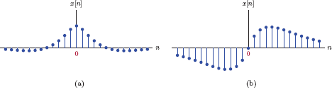
(a) Discrete-time signal with even symmetry, (b) discrete-time signal with odd symmetry.
Decomposition into even and odd components
As in the case of continuous-time signals, any real-valued discrete-time signal x[n]can be written as the sum of two signals, one with even symmetry and one with odd symmetry. The signal x[n] does not have to have any symmetry properties for this to work. Consider the following representation of the signal x[n]:
The signal xe[n] is the even component defined as
and xo[n] is the odd component defined as
It can easily be verified that xe[−n] = xe[n] and xo[−n] = −xo[n]. Furthermore, the signals xe[n]and xo[n] always add up to x[n] owing to the way they are defined.
Symmetry properties for complex signals
Even and odd symmetry definitions given by Eqns. (1.189) and (1.190) for a real-valued signal x[n] can be extended to apply to complex-valued signals as well. A complex-valued signal x[n] is conjugate symmetric if it satisfies
for all n. Similarly, x[n] is conjugate antisymmetric if it satisfies
for all n. If x[n] is conjugate symmetric, time reversing it has the same effect as conjugating it. For a conjugate antisymmetric x[n], time reversal is equivalent to conjugation and negation applied simultaneously.
If the signal x[n] is real-valued, then its complex conjugate is equal to itself, that is, x*[n] = x[n]. In this case the definition of conjugate symmetry reduces to that of even symmetry as can be seen from Eqns. (1.194) and (1.189). Similarly, conjugate antisymmetry property reduces to odd symmetry for a real-valued x[n].
Decomposition of complex signals
Any complex signal x[n] can be expressed as the sum of two signals of which one is conjugate symmetric and the other is conjugate antisymmetric. The component xE[n] defined as
is always conjugate symmetric, and the component xO[n] defined as
is always conjugate antisymmetric. The relationship
holds due to the way xE[n] and xO[n] are defined.
1.5 Further Reading
[1] A.B. Carlson and P.B. Crilly.Communication Systems. McGraw-Hill, 2009.
[2] R.P. Kanwal.Generalized Functions: Theory and Applications. Birkhèauser, 2004.
[3] P. Prandoni and M. Vetterli.Signal Processing for Communications. Communication and Information Sciences. Taylor & Francis, 2008.
[4] A. Spanias, T. Painter, and V. Atti.Audio Signal Processing and Coding. Wiley, 2006.
[5] M. Tohyama.Sound and Signals. Signals and Communication Technology. Springer, 2011.
[6] U. Zölzer.Digital Audio Signal Processing. Wiley, 2008.
MATLAB Exercises
MATLAB Exercise 1.1: Computing and graphing continuous-time signals
Often we have the need to simulate mathematical models of signals on a computer. Sometimes this is done to check the results of hand calculations involving a signal, or to gain graphical insight into signal behavior. At other times we may need a numerical approximation to the mathematical model of a signal for use in a simulation study involving a signal-system interaction problem. In this exercise we will explore methods of computing and graphing continuous-time signal models in MATLAB.
Caveat: Since any row or column vector must have a finite-number of elements, a completely accurate representation of a continuous-time signal is not possible in MATLAB. The best we can do is to approximate a continuous-time signal by constructing a vector that holds amplitudes of the signal at equally-spaced time instants. If the vector used for this purpose has a sufficient number of amplitude values, and if the time spacing of these amplitude values is chosen carefully,9 the result can still be a reasonably good approximation to a continuous-time signal. In graphing such a signal, the signal amplitudes are connected with straight lines to give the appearance of a continuous-time signal.
Compute the signal
at 500 points in the time interval 0 ≤ t ≤ 5, and graph the result.
Solution: Type the following three lines into MATLAB command window to obtain the graph in Fig. 1.87.
>> t = linspace (0,5,500);>> x1 = 5*sin (12*t);>> plot (t,x1);Compute and graph the signal
in the time interval 0 ≤ t ≤ 5 seconds, using a time increment of Δt = 0.01 seconds.
Solution: This signal can be computed and graphed with the following statements:
>> t = [0:0.01:5];>> x2 = exp (-3*t)- exp (-6*t);>> plot (t, x2);The first line demonstrates an alternative method of constructing a time vector. The result is shown in Fig. 1.88.
Compute and graph the signal
in the time interval −2 ≤ t ≤ 3 seconds, using a time increment of Δt = 0.01 seconds.
Solution: The signal we need to graph is the same as the signal in part (b). The slight complication presented by this exercise is due the fact that we need to graph the signal starting at a negative time instant, and signal amplitudes are equal to zero for negative values of t. As a result, two separate descriptions of the signal need to be utilized, one for t < 0 and the other for t ≥ 0. In part (b) we avoided this problem by graphing the signal only for positive values of t and thus using a single analytical expression to compute all signal amplitudes.
The simplest method of dealing with this problem is to use the logic operator “>=” which stands for “greater than or equal to”. The following lines produce the graph shown in Fig. 1.89.
>> t = [-2:0.01:3];>> w = (t>=0);>> x2 = (exp (-3* t)-exp (-6*t)).* w;>> plot (t, x2);Common mistake: It is important to use the element-by-element multiplication operator “.*” and not the vector multiplication operator “*” in the third line above. The expression for computing the vector “x2” involves two vectors of the same size, namely “(exp(-3*t)-exp(-6*t))” and “w”. The operator “.*” creates a vector of the same size by multiplying the corresponding elements of the two vectors. The operator “*”, on the other hand, is used for computing the scalar product of two vectors, and would not work in this case.
-
in the time interval −2 ≤ t ≤ 3 seconds, using a time increment of Δt = 0.01 seconds.
Solution: This signal is similar to the one in part (c). The only difference is that x3 (t) = 0 for t > 1. The logical test needs to be modified to reflect this. Using the logical and operator “&” we can type the following lines into MATLAB command window to compute and graph x3 (t):
>> t = [-2:0.01:3];>> x3 = (exp(-3* t)-exp(-6*t)).*((t>=0)&(t<=1));>> plot (t, x3);The resulting graph is shown in Fig. 1.90.
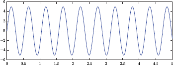
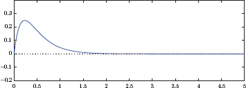

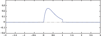
Software resources:
matex_1_1a.m
matex_1_1b.m
matex_1_1c.m
matex_1_1d.m
MATLAB Exercise 1.2: Describing signals using piecewise linear segments
Consider the signal x(t) obtained in Example 1.1 and shown in Fig. 1.8. A signal such as this one can also be described by specifying the endpoints of linear segments and interpolating between them. MATLAB function interp1(..) is used for this purpose.
The endpoints of the signal under consideration are
The code below computes the signal for −1 ≤ t ≤ 6 and graphs the result.
>> tp = [-1,0,1,3,4,5,6];
>> xp = [0,0,1, -1, -1,0,0];
>> t = [-1:0.01:6];
>> x = interp1 (tp, xp, t, ’linear ’);
>> plot (t, x,’b -’, tp, xp, ’ro ’); grid ;
Caution: The function interp1(..) requires that all tp values be distinct, that is, no two points could have the same time value. As a result, signals that have discontinuities (vertical edges) cannot be graphed using this approach.
matex_1_2.m
MATLAB Exercise 1.3: Signal operations for continuous-time signals
In MATLAB Exercise 1.1 we have used vectors for representing mathematical models for continuous-time signals. This approach is often useful for simulating signal-system interaction problems, and will be utilized extensively in later parts of this textbook. In this exercise, however, we will consider alternative approaches for representing signals in MATLAB for the purpose of experimenting with signal operations such as time shifting, time scaling and time reversal.
Consider again the signal x(t) used in Example 1.3 and shown in Fig. 1.16. Analytically x(t) can be written in the form
The following three lines of code create a vector “x” to represent this signal and graph it.
>> t = [-10:0.01:10];
>> x = 2*((t>=-1)&(t<2))+1*((t>=2)&(t <3))-0.5*((t>=3)&(t<=6));
>> plot (t, x);
Since “x” is a vector, there is no easy way to compute and graph the signals g(t) = x (2t − 5) and h(t) = x(−4t + 2) that were graphed in Example 1.3. Instead of using a vector, we will change our strategy, and use a MATLAB function to represent the signal. Create an ASCII text file named “sigx.m” in the current directory and place the following two lines in it:
function x = sigx (t)
x = 2*((t>=-1)&(t<2))+1*((t>=2)&(t<3))-0.5*((t>=3)&(t<=6));
The result is a MATLAB function sigx(..) that returns the value of the signal x(t) at any specified time instant, or even at a set of specified time instants. A vector “g” that holds the amplitude values for the signal g(t) = x (2t − 5) can be computed and graphed with the following set of statements:
>> t = [-10:0.01:10];
>> g = sigx (2*t-5);
>> plot (t, g);
The graph that results should match Fig. 1.17(c). Similarly, a vector “h” with amplitude values of the signal h(t) = x(−4t + 2) can be computed and graphed with the statements
>> t = [-10:0.01:10];
>> h = sigx (-4*t+2);
>> plot (t, h);
The graph produced should match Fig. 1.18(c).
Use of the function sigx(..) allows us to write signal operations in a natural form. One slight drawback is that it requires the creation of an ASCII file “sigx.m” on disc with the function code in it. This may not always be desirable, especially if the signal x(t) will only be used for one exercise and will not be needed again. An alternative method is to create an anonymous function that does not need to be saved into a file. An anonymous function is created for the current MATLAB session, and stays in memory as long as MATLAB remains active. It is discarded when MATLAB is closed. The following statement creates an anonymous function with the name “sx” that works the same way as the function sigx(..):
>> sx = @(t) 2*((t>=-1)&(t <2))+1*((t>=2)&(t<3))-0.5*((t>=3)&(t<=6));
Signals g(t) and h(t) can now be computed and graphed using
>> plot (t,sx(2*t-5));
>> plot (t,sx(-4*t+2));
Software resources:
matex_1_3a.m
matex_1_3b.m
matex_1_3c.m
matex_1_3d.m
sigx.m
MATLAB Exercise 1.4: Creating periodic signals
MATLAB has a number of functions for creating specific periodic waveforms. In this exercise we will explore functions square(..) and sawtooth(..). Afterwards, we will present a simple technique for creating arbitrary periodic waveforms.
One period of a square-wave signal is defined as
MATLAB function square(..) produces a square wave signal with period equal to T = 2π by default, so we need to use time scaling operation to obtain it with any other value of T. The code below will compute and graph a square wave with period T = 1 s for the time interval −1 < t < 10 s.
>> t = [-1:0.01:10];>> x = square (2*pi*t);>> plot (t, x);A square-wave signal with a duty cycle of 0 < d ≤ 1 is defined as
The following code will compute and graph a square-wave signal with period T = 1 s and duty cycle d = 0.2 (or 20 percent).
>> x = square (2*pi*t,20);>> plot (t,x);The function sawtooth(..) generates a sawtooth waveform with period T = 2π. Its definition for one period is
The code below can be used for obtaining a sawtooth signal with period T = 1.5 s.
>> x = sawtooth (2* pi *t /1.5);>> plot (t, x);A signal x(t) that is periodic with period T = 2.5 s is defined through the following:
The following can be used for graphing this signal in the time interval −2 < t < 12 s.
>> t = [-2:0.01:12];>> x1 = @(t)t.*((t>=0)&(t<1))+exp(-5*(t-1)).*((t>=1)&(t<2.5));>> x = x1(mod(t,2.5));>> plot (t, x); grid;The strategy is straightforward: We first create an anonymous function “x1”to describe one period of the signal. In the next line we use that anonymous function with the argument mod(t,2.5) to cause periodic repetition.
Software resources:
matex_1_4a.m
matex_1_4b.m
matex_1_4c.m
matex_1_4d.m
MATLAB Exercise 1.5: Functions for basic building blocks
It is possible to extend MATLAB by developing custom functions for performing tasks that are encountered often. In this exercise we will develop a few simple functions for the computation of basic signal building blocks described in Section 1.3.2.
The unit-step function can be implemented by creating a text file with the name “ss step.m” and the following two lines in it:
1 function x = ss_step (t)
2 x = 1*(t>=0);
It returns the amplitude values for the unit-step function evaluated at each time instant specified by the vector “t”. The unit-ramp function can be implemented with the following two lines saved into a text file named “ss ramp.m”:
1 function x = ss_ramp (t)
2 x = t.*(t>=0);
Functions for computing a unit pulse and a unit triangle can be developed based on the functions ss_step(..) and ss_ramp(..). We will obtain the unit pulse by applying Eqn. (1.36) as follows:
1 function x = ss_pulse (t)
2 x = ss_step (t+0.5) - ss_step (t-0.5);
Similarly, a unit triangle can be obtained by the application of Eqn. (1.43):
1 function x = ss_tri (t)
2 x = ss_ramp (t+1)-2*ss_ramp(t)+ss_ramp(t-1);
Software resources:
matex_1_5.m
ss_step.m
ss_ramp.m
ss_pulse.m
ss_tri.m
MATLAB Exercise 1.6: Computing and graphing discrete-time signals
In previous exercises we have graphed continuous-time signals through the use of the plot(..) function which connects dots with straight lines so that the visual effect is consistent with a signal defined at all time instants. When we work with discrete-time signals we will use a stem plot to emphasize the discrete-time nature of the signal.
Compute and graph the signal
for the range of the sample index 4 ≤ n ≤ 8.
Solution: Type the following three lines into MATLAB command window to obtain the graph shown in Fig. 1.91.
>> n = [4:8];>> x1 = [1.1, 2.5, 3.7, 3.2, 2.6];>> stem (n,x1);Compute and graph the signal
for the index range n = 0, 1,..., 99.
Solution: This signal can computed and graphed with the following statements:
>> n = [0:99];>> x2 = sin(0.2*n);>> stem (n,x2);The result is shown in Fig. 1.92.
Compute and graph the signal
for the interval n = −20,..., 59.
Solution: The signal x3[n] to be graphed is similar to the signal of part (b), but is a finite-length signal that equals zero for n < 0 and for n > 39. As in MATLAB Exercise 1.1 we will solve this problem by using logic operators on the index vector “n”. Type the following statements into the command window to compute and graph the signal x3[n].
>> n = [-20:59];>> x3 = sin (0.2*n).*((n>=0)&(n<=39));>> stem (n,x3);The result is shown in Fig. 1.93.
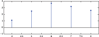

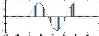
Software resources:
matex_1_6a.m
matex_1_6b.m
matex_1_6c.m
MATLAB Exercise 1.7: Periodic extension of a discrete-time signal
Sometimes a periodic discrete-time signal is specified using samples of one period. Let x[n] be a length-N signal with samples in the interval n = 0,...,N − 1. Let us define the signal as the periodic extension of x[n] so that
In this exercise we will develop a MATLAB function to periodically extend a discrete-time signal. The function ss_per(..) given below takes a vector “x” that holds one period (N samples) of x[n]. The second argument “idx” is a vector that holds the indices at which the periodic extension signal should be evaluated. The samples of the periodic signal x[n] are returned in the vector “xtilde”.
1 function xtilde = ss_per (x, idx)
2 N = length (x); % Period of the signal.
3 n = mod (idx, N); % Modulo indexing.
4 nn = n+1; % MATLAB indices start with 1.
5 xtilde = x(nn);
6 end
Consider a length-5 signal x[n] given by
The periodic extension can be computed and graphed for n = −15,...,15 with the following statements:
>> x = [0,1,2,3,4]
>> n = [-15:15]
>> xtilde = ss_per (x, n)
>> stem (n, xtilde)
What if we need to compute and graph a time reversed version in the same interval? That can also be accomplished easily using the following statements:
>> xtilde = ss_per (x,-n)
>> stem (n, xtilde)
Software resources:
matex_1_7.m
ss_per.m
Problems
1.1. Sketch and label each of the signals defined below:
1.2. Consider the signals shown in Fig. P.1.2. For each signal write the analytical description in segmented form similar to the descriptions of the signals in Problem 1.1.
1.3. Using the two signals xa (t) and xb (t) given in Fig. P.1.2, compute and sketch the signals specified below:
- g1 (t) = xa (t) + xb (t)
- g2 (t) = xa (t) xb (t)
- g3 (t) = 2xa (t) − xb (t) + 3
1.4. For the signal x(t) shown in Fig. P.1.4, compute the following:
- g1 (t) = x(−t)
- g2 (t) = x (2t)
- g4 (t) = x(−t + 3)
- g6 (t) = x (4t − 3)
-
Determine and sketch the following signals derived from x(t) through signal operations:
1.6. Let b be a positive constant. Show that
Hint: Start with Eqn. (1.23) that expresses the impulse function as the limit of a pulse q(t) with height 1/a and unit area. Apply time scaling to q(t) and then take the limit as a → 0.
1.7. Consider again Eqn. (1.23) that expresses the impulse function as the limit of a pulse q(t) with height 1/a and area equal to unity. Show that, for small values of a, we have
where f(t) is any function that is continuous in the interval t1 − a/2 < t < t1 + a/2. Afterwards, by taking the limit of this result, show that the sifting property of the impulse function holds.
1.8. Sketch each of the following functions.
- δ(t) + δ(t − 1) + δ(t − 2)
- −(t − 1) + u(t)
- e−t δ (t − 1)
- e−t [u(t − 1) − u(t − 2)]
1.9. Sketch each of the following functions in the time interval −1 ≤ t ≤ 5. Afterwards use the waveform explorer program “wav_demo1.m” to check your results.
- u(t) + u(t − 1) − 3u(t − 2) + u(t − 3)
- r(t) − 2r(t − 2) + r(t − 3)
- u(t) + r(t − 2) − u(t − 3) − r(t − 4)
- Λ(t) + 2Λ(t − 1) + 1.5Λ (t − 3) − Λ(t − 4)
1.10. Express each of the signals shown in Fig. P.1.10 using scaled and time shifted unit-step functions. Afterwards use the waveform explorer program “wav_demo1.m” to check your results.
1.11. Consider again the signals in Fig. P.1.10. Express each signal using scaled and time shifted unit-pulse functions. Afterwards use the waveform explorer program “wav_demo1.m” to check your results.
1.12. Express the signal x(t) shown in Fig. P.1.12 using
- Unit-ramp functions
- Unit-triangle functions
In each case, check your results using the waveform explorer program “wav_demo1.m”.
1.13. Suppose that in an experiment we collect data in the form of (ti, xi) pairs for i = 1,...,N, and would like to construct a continuous-time signal x(t) by linear interpolation, that is, by connecting the points with straight line segments as shown in Fig. P.1.13(a). The only restriction is that all ti values are distinct; no two data points have the same time value. Let us define a skewed triangle function in the form
which is shown in Fig. P.1.13(b). Devise a method of expressing the linearly interpolated signal x(t) in terms of the skewed triangle functions.
1.14. Time derivative of the unit-impulse function δ(t) is called a doublet. Given a function f(t) that is continuous at t = 0 and also has continuous first derivative at t = 0, show that
Hint: Use integration by parts, and then apply the sifting property of the impulse function.
1.15. Signum function is defined as
Express the function sgn (t) in terms of the unit-step function.
1.16. Using Euler’s formula, prove the following identities:
- cos (a + b) = cos(a) cos(b) − sin (a) sin (b)
- sin (a + b) = sin (a) cos (b) + cos (a) sin (b)
1.17. Using the definition of periodicity, determine if each signal below is periodic or not. If the signal is periodic, determine the fundamental period and the fundamental frequency.
- x(t) = 3 cos (2t + π/10)
- x(t) = 3 cos(2t + π/10) u(t)
- x(t) = cos2 (3t − π/3)
- x(t) = e−|t| cos (2t)
- x(t) = ej(2t+π/10)
- x(t) = e(−1+j2)t
1.18. Determine the periodicity of each of the multi-tone signals given below. For those that are periodic, determine the fundamental period and the fundamental frequency.
- x(t) = 2 cos(5t + π/ 10) + 3 sin (5πt)
- x(t) = cos(10πt) − 3 sin (30πt + π/4)
- x(t) = cos (45πt) + cos(55πt)
1.19. A signal g(t) is defined in terms of another signal x(t) as
- If x(t) is an energy signal with normalized energy equal to Ex, show that g(t) is also an energy signal. Determine the normalized energy of g(t) in terms of Ex and A.
- If x(t) is a power signal with normalized average power equal to Px, show that g(t) is also a power signal. Determine the normalized average power of g(t) in terms of Px and A.
1.20. A signal g(t) is defined in terms of another signal x(t) as
- If x(t) is an energy signal with normalized energy equal to Ex, is g(t) is an energy signal or a power signal?
- Determine either the normalized energy or the normalized average power of g(t) as appropriate, in terms of Ex, A and B.
1.21. Determine the normalized energy of each of the signals given below.
- x(t) = e −2|t|
- x(t) = e−2t u(t)
- x(t) = e −2t cos (5t)u (t)
Hint: Express the cosine term in x(t) using Euler’s formula prior to squaring and integrating.
1.22. Determine the normalized energy of each of the signals shown in Fig. P.1.2.
1.23. Determine the normalized average power of each of the periodic signals shown in Fig. P.1.23.
1.24. In Example 1.12 the RMS value of a multi-tone signal was derived for the case of distinct frequencies. Now consider the signal
where the first two terms have the same frequency. Determine the RMS value of the signal.
1.25. Identify which of the signals in Fig. P.1.25 are even, which ones are odd, and which signals are neither even nor odd.
1.26. Consider a signal x(t). Show that
- If x(t) is even, then
- If x(t) is odd, then
- If x(t) is even, then
1.27. Let x(t) = x1 (t)x2 (t). Show that
- If both x1 (t) and x2 (t) are even, then x(t) is even.
- If both x1 (t) and x2 (t) are odd, then x(t) is even.
- If both x1 (t) is even and x2 (t) is odd, then x(t) is odd.
1.28. Determine the conjugate symmetric and conjugate antisymmetric components of the signal x(t) = e(−2+j10π)t. Sketch each component in polar form, that is, in terms of its magnitude and phase.
1.29. For each of the signals listed below, find the even and odd components xe (t) and xo (t). In each case, sketch the original signal and its two components.
- x(t) = e −5t sin (t)u(t)
- x(t) = e−3|t| cos (t)
- x(t) = e−3|t| sin (t)
- x(t) = te−3t + 2 u(t)
- x(t) = e−2|t−1|
1.30. Determine and sketch even and odd components of the signal x(t) used in Problem 1.12 and shown in Fig. P.1.12.
1.31. Transform each of the sinusoidal signals given below into phasor form.
- x(t) = 3 cos (200πt)
- x(t) = 7 sin (100πt)
- x(t) = 2 sin (10πt) − 5 cos (10πt)
1.32. Using an operating frequency of f0 = 10 Hz, express the phasors given below as time-domain signals.
- X =5ej14°
- X =2ej28° + 3 ej18°
- X =2ej28° − 3ej18°
1.33. For the signal x[n] shown in Fig. P.1.33, sketch the following signals.
1.34. Consider the sinusoidal discrete-time signal
Is the signal periodic? If yes, determine the fundamental period.
1.35. Carefully sketch each signal described below.
- x[n] = (0.8)n u[n]
- x[n] = u [n] − u[n − 10]
- x[n] = r[n] − 2r[n − 5] + r [n − 10]
1.36. Determine the normalized energy of each signal described in Problem 1.35.
1.37. Consider a signal x[n]. Show that
- If x[n] is even, then
- If x[n] is odd, then
1.38. Let x[n] = x1[n]x2[n]. Show that
- If both x1[n] and x2[n] are even, then x[n] is even.
- If both x1[n] and x2[n] are odd, then x[n] is even.
- If x1[n] is even and x2[n] is odd, then x[n] is odd.
1.39. Determine even and odd components of the signal x[n] shown in Fig. P.1.39.
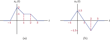
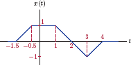
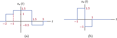
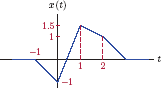
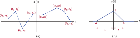
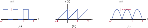
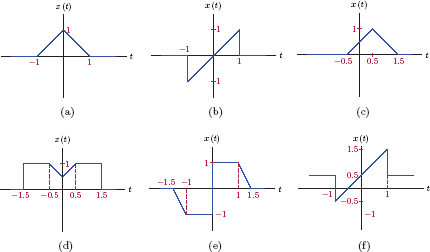
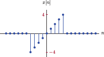

MATLAB Problems
1.40. Write a MATLAB script to compute and graph the signals xa (t) and xb (t) described in Problem 1.1. Use an anonymous function for each signal based on the analytical description given (see MATLAB Exercise 1.1). Graph each signal in the interval − 1 ≤ t ≤ 6 with a time increment of Δt = 0.01. Label the axes appropriately.
-
- Consider the signals xa (t) and xb (t) described in Problem 1.2. Using the interp1(..) function of MATLAB, compute each signal in the time interval −2 ≤ t ≤ 4 with a time increment of Δt = 0.01 (see MATLAB Exercise 1.2).
- Afterwards, compute the signals g1 (t), g2 (t) and g3 (t) from the signals xa (t) and xb (t) as specified in Problem 1.3. Graph each signal in the same time interval as in part (a). Carefully label the axes of each graph.
1.42. Refer to the signals g1 (t) and g2 (t) found in Example 1.2 and shown in Fig. 1.12. Develop a MATLAB script to verify the analytical forms of these signals given by Eqns. (1.5) and (1.6). Your script should
- Compute samples of each signal in the time interval − 1 ≤ t ≤4 using a time increment of Δt = 0.01 s.
- Graph the results using the “subplot” function.
Ensure that the computations in part (a) correspond directly to Eqns. (1.5) and (1.6).
1.43. Refer to the signal x(t) used in Problem 1.4 and shown in Fig. P.1.4.
- Express the signal x(t) through the use of a MATLAB anonymous function that utilizes the function interp1(..).
- Using MATLAB, compute and graph each of the signals for parts (a) through (g) of Problem 1.4 in the time interval − 10 < t < 10 s, using a time increment of Δt =0.02 s. Compare MATLAB graphs to those obtained manually in Problem 1.4.
1.44. Refer to the signal x(t) used in Problem 1.5.
- Express the signal x(t) through the use of a MATLAB anonymous function.
- Using MATLAB, compute and graph each of the signals for parts (a) through (d) of Problem 1.5 in the time interval − 10 < t < 10 s, using a time increment of Δt = 0.02s. Compare MATLAB graphs to those obtained manually in Problem 1.5.
1.45. Using MATLAB functions ss_step(..), ss_ramp(..), ss_pulse(..) and ss_tri(..) developed in MATLAB Exercise 1.5, graph each of the signals specified in Problem 1.9 parts (a) through (e) in the time interval − 2 < t <8 s, using a time increment of Δt = 0.01 s. Compare MATLAB graphs to those obtained manually in Problem 1.9.
1.46. Consider the signal x(t) used in Problem 1.12 and graphed in Fig. P.1.12.
- Express this signal through an anonymous MATLAB function that utilizes the function ss_ramp(..), and graph the result in an appropriate time interval.
- Repeat part (a) using the function ss_tri(..) instead of the function ss_ramp(..).
- In MATLAB, compute and graph even and odd components of the signal x(t). Code Eqns. (1.109) and (1.110) directly in MATLAB for this purpose. Compare your MATLAB graphs to those obtained manually in Problem 1.30.
1.47. Consider the discrete-time signal x[n] used in Problem 1.33 and graphed in Fig. P.1.33.
- Express this signal through an anonymous MATLAB function that utilizes the function ss_ramp(..), and graph the result for index range n = − 10,..., 10.
- Express each of the signals in parts (a) through (h) of Problem 1.33 in MATLAB, and graph the results. Use functions ss_step(..) and ss_ramp(..) as needed.
1.48. Consider the discrete-time signal x[n] used in Problem 1.39 and graphed in Fig. P.1.39.
- Express this signal through an anonymous MATLAB function that utilizes the function ss_ramp(..), and graph the result for index range n = − 10,..., 10.
- Write a script to compute and graph even and odd components of this signal.
MATLAB Projects
1.49. In Problem 1.13 a method was developed for linearly interpolating between data points (ti, xi) for i = 1,..., N using the skewed triangle function shown in Fig. P.1.13b.
Write a MATLAB function ss_trs(..) to compute values of the skewed triangle function at time instants specified in vector “t”. The function should have the syntax
x = ss_trs (t, a, b)where “t” is a row vector. Arguments “a” and “b” are both positive scalars. Test your function to compute and graph the functions Λs (t, 3, 2), Λs (t, 1, 4), and Λs (t, 2.7, 1.3) in the time interval − 5 ≤ t ≤ 5 using a time increment Δt = 0.01.
Next, write a MATLAB function ss_interp(..) to interpolate between a set of data points. The function should have the syntax
x = ss_interp (tvec, xvec, t)The arguments “tvec” and “xvec” are row vectors of equal length. The vector “tvec” holds t1,..., tN, and the vector “xvec”holds x1,..., xN. The returned vector “x” holds values of the interpolated signal at time instants specified in the vector “t”.
Write a MATLAB script to test the function ss_interp(..) with the set of data points
Graph the interpolated signal in the time interval − 4 ≤ t ≤ 5 using a time increment of Δt = 0.01.
1.50. In some digital systems such as inexpensive toys, sinusoidal signals at specific frequencies may be generated through table look-up, thus eliminating the need for the system to include the capability to compute trigonometric functions. Samples corresponding to exactly one period of the sinusoidal signal are computed ahead of time and stored in memory. When the signal is needed, the contents of the look-up table are played back repeatedly. Consider a sinusoidal signal
with f1 = 1336 Hz. Let x1[n] be a discrete-time sinusoidal signal obtained by evaluating xa (t) at intervals of 125 μs corresponding to a sampling rate of 8000 samples per second.
Determine the fundamental period N1 for the signal x1[n].
Write a MATLAB script to accomplish the following:
- - Create a vector “x1” that holds exactly one period of the signal.
- - By repeating the vector “x1” as many times as needed, create a vector “x”that holds 8000 samples of the sinusoidal signal that corresponds to a time duration of 1 second.
- - Play back the resulting sound using the sound(..) function of MATLAB. If the fundamental period was computed properly in part (a) then the repeated sections of the signal should fit together seamlessly, and you should hear a clean tone.
Modify the script in part (b) so that the number of samples used in creating the vector “x1” is 10 less than the correct value found in part (a). Create a vector “x”by repeating this imperfect vector “x1” as many times as necessary. Listen to the audio playback of the vector “x”, and comment on the difference. Also, graph the resulting signal. Using the zoom tool, zoom into the transition area between two repetitions, and observe the flaw in the transition that is due to incorrect period length.
Repeat parts (a) through (c) using the sinusoidal signal
with f1 = 852 Hz, and the corresponding discrete-time signal
Consider the dual-tone signal
Using the table look-up method with the vectors “x1” and “x2” obtained above, generate a vector that holds 8000 samples of the dual-tone signal. Play back the resulting vector and comment.
1.51. In this project the concept of dual-tone multi-frequency (DTMF) signaling will be explored. As the name implies, DTMF signals are mixtures of two sinusoids at distinct frequencies. They are used in communications over analog telephone lines. A particular version of DTMF signaling is utilized in dialing a number with push-button telephone handsets, a scheme known as touch tone dialing. When the caller dials a number, the DTMF generator produces a dual-tone signal for each digit dialed. The synthesized signal is in the form
Frequency assignments for the digits on a telephone keypad are shown in Fig. P.1.51.
The goal of this project is to develop a DTMF synthesizer function for MATLAB.
Develop a function named ss_dtmf1(..) to produce the signal for one digit. The syntax of the function should be
x = ss_dtmf1(n,t)The first argument “n” is the digit for which the DTMF signal is to be generated. Let values n = 0 through n = 9 represent the corresponding keys on the keypad. Map the remaining two keys “*” and “#” to values n = 10 and n = 11 respectively. Finally, the value n = 12 should represent a pause, that is, a silent period. The vector “t” contains the time instants at which the DTMF signal x(t) is evaluated and returned in vector “x”.
Develop a function named ss_dtmf(..) with the syntax
x = ss_dtmf (number, dt, nd, np)The arguments for the function ss_dtmf(..) are defined as follows:
number: The phone number to be dialed, entered as a vector. For example, to dial the number 555-1212, the vector “number” would be entered as
number = [5,5,5,1,2,1,2]dt: The time increment Δt to be used in computing the amplitudes of the DTMF signal.
nd: Parameter to control the duration of the DTMF signal for each digit. The duration of each digit should be
np: Parameter to control the duration of pause between consecutive digits. The duration of pause should be
The function ss_dtmf(..) should use the function ss_dtmf1(..) to produce the signals xk (t) for each digit (and the pauses between digits) and append them together to create the signal x(t).
Write a script to test the function ss_dtmf(..) with the number 555-1212. Use a time-increment of 125 microseconds corresponding to 8000 values per second. The duration of each digit should be 200 milliseconds with 80 millisecond pauses between digits.
Play back the resulting signal x(t) using the sound(..) function.
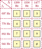
1 A thorough mathematical study of singularity functions such as the unit-impulse function is quite advanced, and is well beyond the scope of this text. From a theoretical standpoint, one could set up conditions under which the sampling property given by Eqn. (1.26) may not hold. However, it will be valid and useful for our purposes in formulating signal models for engineering applications.
2 It should be noted that we are not aiming for a mathematically rigorous proof here, but rather some insight. We are assuming that x(t) is a well behaving function that allows the limit in Eqn. (1.54).
3 e±ja = cos(a)± j sin (a).
4 cos2 (a) + sin2 (a) = 1, and tan (a) = sin(a) / cos (a).
5 .
6 .
7 cos (a + b) = cos(a) cos (b) − sin (a) sin (b).
8 eja = cos(a) + j sin(a).
9 A more formal method of determining the appropriate time spacing for signal amplitude values will be given when we discuss the subject of sampling in Chapter 6.