
Analyzing Continuous-Time Systems in the Time Domain
Chapter Objectives
- Develop the notion of a continuous-time system.
- Learn simplifying assumptions made in the analysis of systems. Discuss the concepts of linearity and time invariance, and their significance.
- Explore the use of differential equations for representing continuous-time systems.
- Develop methods for solving differential equations to compute the output signal of a system in response to a specified input signal.
- Learn to represent a differential equation in the form of a block diagram that can be used as the basis for simulating a system.
- Discuss the significance of the impulse response as an alternative description form for linear and time-invariant systems.
- Learn how to compute the output signal for a linear and time-invariant system using convolution. Understand the graphical interpretation of the steps involved in carrying out the convolution operation.
- Learn the concepts of causality and stability as they relate to physically realizable and usable systems.
2.1 Introduction
In this chapter, we will begin our examination of the system concept. An overly simplified and rather broad definition of a system may be given as follows:
In general, a system is any physical entity that takes in a set of one or more physical signals and, in response, produces a new set of one or more physical signals.
Consider a microphone that senses the variations in air pressure created by the voice of a singer, and produces a small electrical signal in the form of a time-varying voltage. The microphone acts as a system that facilitates the conversion of an acoustic signal to an electrical signal. Next, consider an amplifier that is connected to the output terminals of the microphone. It takes the small-amplitude electrical signal from the microphone, and produces a larger-scale replica of it suitable for use with a loudspeaker. Finally a loudspeaker that is connected to the output terminals of the amplifier converts the electrical signal to sound. We can view each of the physical entities, namely the microphone, the amplifier and the loudspeaker, as individual systems. Alternatively, we can look at the combination of all three components as one system that consists of three subsystems working together.
Another example is the transmission of images from a television studio to the television sets in our homes. The system that achieves the goal of bringing sound and images from the studio to our homes is a rather complex one that consists of a large number of subsystems that carry out the tasks of 1) converting sound and images to electrical signals at the studio, 2) transforming electrical signals into different formats for the purposes of enhancement, encoding and transmission, 3) transmitting electrical or electromagnetic signals over the air or over a cable connection, 4) receiving electrical or electromagnetic signals at the destination point, 5) processing electrical signals to convert them to formats suitable for a television set, and 6) displaying the images and playing the sound on the television set. Within such a large-scale system some of the physical signals are continuous-time signals while others are discrete-time or digital signals.
Not all systems of interest are electrical. An automobile is an example of a large-scale system that consists of numerous mechanical, electrical and electromechanical subsystems working together. Other examples are economic systems, mass transit systems, ecological systems and computer networks. In each of these examples, large-scale systems are constructed as collections of interconnected smaller-scale subsystems that work together to achieve a prescribed goal.
In this textbook we will not attempt a complete treatment of any particular large-scale system. Instead, we will focus our efforts on developing techniques for understanding, analyzing and designing subsystems with accurate and practical models based on laws of physics and mathematical transforms. In general, a system can be viewed as any physical entity that defines the cause-effect relationships between a set of signals known as inputs and another set of signals known as outputs. The input signals are excitations that drive the system, and the output signals are the responses of the system to those excitations.
In Chapter 1 we have discussed basic methods of mathematically modeling continuous-time and discrete-time signals as functions of time.
The mathematical model of a system is a function, formula or algorithm (or a set of functions, formulas, algorithms) to approximately recreate the same cause-effect relationship between the mathematical models of the input and the output signals.
If we focus our attention on single-input/single-output systems, the interplay between the system and its input and output signals can be graphically illustrated as shown in Fig. 2.1.

If the input and the output signals are modeled with mathematical functions x(t) and y(t) respectively, then the system itself needs to be modeled as a function, formula, or algorithm of some sort that converts the signal x(t) into the signal y(t). Sometimes we may have the need to design a system to achieve a particular desired effect in the conversion of the input signal x(t) to the output signal y(t). For example, an amplifier increases the power level of a signal that may be too weak to be heard or transmitted, while preserving its information content. A frequency-selective filter can be used for either removing or boosting certain frequencies in a signal. A speech recognition system can analyze the signal x(t) in an attempt to recognize certain words, with the goal of performing certain tasks such as connecting the caller to the right person via an automated telephone menu system.
In contrast with systems that we design in order to achieve a desired outcome, sometimes the effect of a particular system on the input signal is not a desired one, but one that we are forced to accept, tolerate, or handle. For example, a wire connection is often used so that a signal that exists at a particular location could be duplicated at a distant remote location. In such a case, we expect the wire connection to be transparent within the scheme of transmitting the signal from point A to point B; however, that is usually not the case. The physical conductors used for the wire connection are far from ideal, and cause changes in the signal as it travels from A to B. The characteristics of the connection itself represent a system that is more of a nuisance than anything else. We may need to analyze this system, and find ways to compensate for the undesired effects of this system if we are to communicate successfully.
The relationship between the input and the output signals of a continuous-time system will be mathematically modeled as
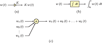
where the operator Sys {...} represents the transformation applied to x(t). This transformation can be anything from a very simple one to a very complicated one. Consider, for example, a system that amplifies its input signal by a constant gain factor K to yield an output signal
or one that delays its input signal by a constant time delay τ to produce
or a system that produces an output signal that is proportional to the square of the input signal as in
In all three examples above, we have system definitions that could be expressed in the form of simple functions. This is not always the case. More interesting systems have more complicated definitions that cannot be reduced to a simple function of the input signal, but must rather be expressed by means of an algorithm, a number of functional relationships interconnected in some way, or a differential equation.
In deriving valid mathematical models for physical systems, we rely on established laws of physics that are applicable to individual components of a system. For example, consider a resistor in an electronic circuit. In mathematically modeling a resistor we use Ohm’s law which states that the voltage between the terminals of a resistor is proportional to the current that flows through it. This leads to the well-known relationship v = Ri between the resistor voltage and the resistor current. On the other hand, laboratory experiments indicate that the resistance of an actual carbon resistor varies as a function of temperature, a fact which is neglected in the mathematical model based on Ohm’s law. Thus, Ohm’s law provides a simplification of the physical relationship involved. Whether this simplification is acceptable or not depends on the specifics of the circuit in which the resistor is used. How significant are the deviations of the mathematical model of the resistor from the behavior of the actual resistor? How significant are the temperature changes that cause these deviations? How sensitive is the circuit to the variations in the value of R ?Answers to these and similar questions are used for determining if the simple mathematical model is appropriate, or if a more sophisticated model should be used. Modeling of a system always involves some simplification of the physical relationships between input and output signals. This is necessary in order to obtain mathematical models that are practical for use in understanding system behavior. Care should be taken to avoid oversimplification and to ensure that the resulting model is a reasonably accurate approximation of reality.
Two commonly used simplifying assumptions for mathematical models of systems are linearity and time invariance which will be the subjects of Section 2.2. Section 2.3 focuses on the use of differential equations for representing continuous-time systems. Restrictions that must be placed on differential equations in order to model linear and time-invariant systems will be discussed in Section 2.4. Methods for solving linear constant-coefficient differential equations will be discussed in Section 2.5. Derivation of block diagrams for simulating continuous-time linear and time-invariant systems will be the subject of Section 2.6. In Section 2.7 we discuss the significance of the impulse response and its use in the context of the convolution operator for determining the output signal of a system. Concepts of causality and stability of systems are discussed in Sections 2.8 and 2.9 respectively.
2.2 Linearity and Time Invariance
In most of this textbook we will focus our attention on a particular class of systems referred to as linear and time-invariant systems. Linearity and time invariance will be two important properties which, when present in a system, will allow us to analyze the system using well-established techniques of the linear system theory. In contrast, the analysis of systems that are not linear and time-invariant tends to be more difficult, and often relies on methods that are specific to the types of systems being analyzed.
2.2.1 Linearity in continuous-time systems
A system is said to be linear if the mathematical transformation y(t) = Sys{x(t)} that governs the input-output relationship of the system satisfies the following two equations for any two input signals x1 (t), x2 (t) and any arbitrary constant gain factor α1.
The condition in Eqn. (2.5) is the additivity rule which can be stated as follows: The response of a linear system to the sum of two signals is the same as the sum of individual responses to each of the two input signals. The condition in Eqn. (2.6) is the homogeneity rule. Verbally stated, scaling the input signal of a linear system by a constant gain factor causes the output signal to be scaled with the same gain factor. The two criteria given by Eqns. (2.5) and (2.6) can be combined into one equation which is referred to as the superposition principle.
Superposition principle:
A continuous-time system is linear if it satisfies the superposition principle stated in Eqn. (2.7) for any two arbitrary input signals x1 (t), x2 (t) and any two arbitrary constants α1 and α2. The superposition principle applied to two signals can be expressed verbally as follows: The response of the system to a weighted sum of two input signals is equal to the same weighted sum of the responses of the system to individual input signals. This concept is very important, and is graphically illustrated in Fig. 2.2.
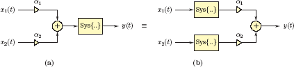
Illustration of Eqn. (2.7). The two configurations shown are equivalent if the system under consideration is linear.
Furthermore, if superposition works for the weighted sum of any two input signals, it can be proven by induction that it also works for an arbitrary number of input signals. Mathematically we have
The generalized form of the superposition principle can be expressed verbally as follows: The response of a linear system to a weighted sum of N arbitrary signals is equal to the same weighted sum of the individual responses of the system to each of the N signals. Let yi (t) be the response to the input component xi (t) alone, that is yi (t) = Sys {xi (t)} for i = 1,..., N. Superposition principle implies that
This is graphically illustrated in Fig. 2.3.
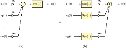
Illustration of Eqn. (2.7). The two configurations shown are equivalent if the system under consideration is linear.
Testing a system for linearity involves checking whether the superposition principle holds true with two arbitrary input signals. Example 2.1 will demonstrate this procedure.
Example 2.1: Testing linearity of continuous-time systems
Four different systems are described below through their input-output relationships. For each, determine if the system is linear or not:
- y(t) = 5x(t)
- y(t) = 5x(t) + 3
- y(t) = 3 [x(t)]2
- y(t) = cos(x(t))
Solution:
If two input signals x1 (t) and x2 (t) are applied to the system individually, they produce the output signals y1 (t) = 5x1 (t) and y2 (t) = 5x2 (t) respectively. Let the input signal be x(t) = α1 x1 (t)+α2x2 (t). The corresponding output signal is found using the system definition:
Superposition principle holds; therefore this system is linear.
If two input signals x1 (t) and x2 (t) are applied to the system individually, they produce the output signals y1 (t) = 5x1 (t) + 3 and y2 (t) = 5x2 (t) + 3 respectively.
We will again use the combined input signalx(t) = α1 x1 (t) + α2 x2 (t) for testing. The corresponding output signal for this system is
The output signal y(t) cannot be expressed in the form y(t) = α1 y1 (t) + α2 y2 (t). Superposition principle does not hold true in this case. The system in part (b) is not linear.
Using two input signals x1 (t) and x2 (t) individually, the corresponding output signals produced by this system are y1 (t) = 3 [x1 (t)]2 and y2 (t) = 3 [x2 (t)]2 respectively. Applying the linear combination x(t) = α1 x1 (t) + α2 x2 (t) to the system produces the output signal
It is clear that this system is not linear either.
The test signals x1 (t) and x2 (t) applied to the system individually produce the output signals y1 (t) = cos[x1 (t)] and y2 (t) = cos[x2 (t)] respectively. Their linear combination x(t) = α1 x1 (t) + α2 x2 (t) produces the output signal
This system is not linear either.
Software resources: |
See MATLAB Exercise 2.1. |
2.2.2 Time invariance in continuous-time systems
Another important concept in the analysis of systems is time invariance. A system is said to be time-invariant if its behavior characteristics do not change in time. Consider a continuous-time system with the input-output relationship
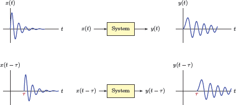
If the input signal applied to a time-invariant system is time-shifted by τ seconds, the only effect of this delay should be to cause an equal amount of time shift in the output signal, but to otherwise leave the shape of the output signal unchanged. If that is the case, we would expect the relationship
to also be valid.
Condition for time-invariance:
This relationship is depicted in Fig. 2.4.
Alternatively, the relationship described by Eqn. (2.10) can be characterized by the equivalence of the two system configurations shown in Fig. 2.5.

Another interpretation of time-invariance. The two configurations shown are equivalent for a time-invariant system.
Testing a system for time invariance involves checking whether Eqn. (2.10) holds true for any arbitrary input signal. This procedure will be demonstrated in Example 2.2.
Example 2.2: Testing time invariance of continuous-time systems
Three different systems are described below through their input-output relationships. For each, determine whether the system is time-invariant or not:
- y(t) = 5x(t)
- y(t) = 3 cos (x(t))
- y(t) = 3 cos(t)x(t)
Solution:
For this system, if the input signal x(t) is delayed by τ seconds, the corresponding output signal would be
and therefore the system is time-invariant.
Let the input signal be x(t − τ). The output of the system is
This system is time-invariant as well.
Again using the delayed input signal x (t − τ) we obtain the output
In this case the system is not time-invariant since the time-shifted input signal leads to a response that is not the same as a similarly time-shifted version of the original output signal.
Before we leave this example we will use this last part of the problem as an opportunity to address a common source of confusion. The question may be raised as to whether the term t in the argument of the cosine function should be replaced with t − τ as well. In other words, should we have written
which would have led to the conclusion that the system under consideration might be time-invariant? The answer is no. The term cos (t) is part of the system definition and not part of either the input or the output signal. Therefore we cannot include it in the process of time shifting input and output signals.
Software resources: |
See MATLAB Exercise 2.2. |
Example 2.3: Using linearity property
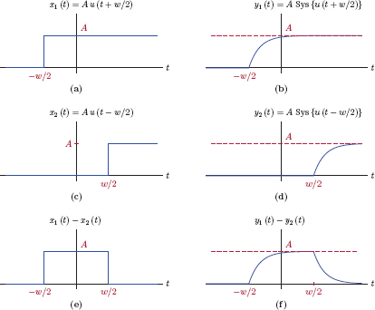
A continuous-time system with input-output relationship y(t) = Sys{x(t)} is known to be linear. Whether the system is time-invariant or not is not known. Assume that the responses of the system to four input signals x1 (t),x2 (t) x3 (t) and x4 (t) shown in Fig. 2.6 are known.
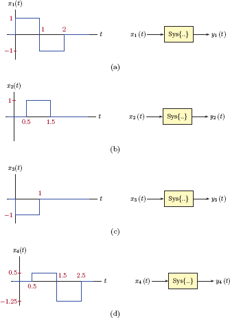
Discuss how the information provided can be used for finding the response of this system to the signal x(t) shown in Fig. 2.7.
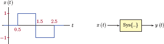
Solution: Through a first glance at the four input signals given we realize that x(t) is a time-shifted version of x1 (t), that is, x(t) = x1 (t − 0.5). As a result, we may be tempted to conclude that y(t) = y1 (t − 0.5), however, this would be the wrong approach since the system is not necessarily time-invariant. We do not know for a fact that the input signal x1 (t − 0.5) produces the response y1 (t − 0.5). For the same reason, we cannot base our solution on the idea of constructing the input signal from x2 (t) and x3 (t) as
since it involves time shifting the signal x3 (t), and we do not know the response of the system to x3 (t − 1.5). We need to find a way to construct the input signal from input signals given, using only scaling and addition operators, but without using any time shifting. A possible solution is to write x(t) as
Since the system is linear, the output signal is
2.2.3 CTLTI systems
In the rest of this textbook, we will work with continuous-time systems that are both linear and time-invariant. A number of time- and frequency-domain analysis and design techniques will be developed for such systems. For simplicity, we will use the acronym CTLTI to refer to continuous-time linear and time-invariant systems.
2.3 Differential Equations for Continuous-Time Systems
One method of representing the relationship established by a system between its input and output signals is a differential equation that approximately describes the interplay of the physical quantities within the system. Such a differential equation typically involves the input and the output signals as well as various derivatives of either or both. Following is an example:
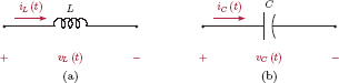
If we need to model a mechanical system with a differential equation, physical relationships between quantities such as mass, force, torque and acceleration may be used. In the case of an electrical circuit we use the physical relationships that exist between various voltages and currents in the circuit, as well as the properties of the circuit components that link those voltages and currents. For example, the voltage between the leads of an inductor is known to be approximately proportional to the time rate of change of the current flowing through the inductor. Using functions νL (t) and iL (t) as mathematical models for the inductor voltage and the inductor current respectively, the mathematical model for an ideal inductor is
Similarly, the current that flows through a capacitor is known to be proportional to the rate of change of the voltage between its terminals, leading to the mathematical model of an ideal capacitor as
where υC (t) and iC (t) are the mathematical models for the capacitor voltage and the capacitor current respectively.
Ideal inductor and the ideal capacitor represent significant simplification of real-life versions of these devices with their physical voltage and current quantities. The following examples will demonstrate the process of obtaining a differential equation from the physical description of a system.
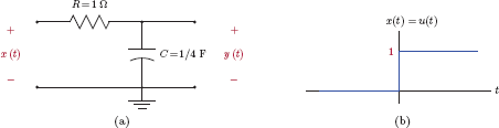
Example 2.4: Differential equation for simple RC circuit
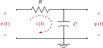
Consider the simple first-order RC circuit shown in Fig. 2.9. The input signal x(t) is the voltage applied to a series combination of a resistor and a capacitor, and the output signal is the voltage y(t) across the terminals of the capacitor.
Even though the RC circuit is a very simple example of a system, it will prove useful in discussing fundamental concepts of linear systems theory, and will be used as the basis of several examples that will follow. The techniques that we will develop using the simple RC circuit of Fig. 2.9 as a backdrop will be applicable to the solution of more complex problems involving a whole host of other linear systems.
It is known from circuit theory that both the resistor and the capacitor carry the same current i(t). Furthermore, the voltage drop across the terminals of the resistor is
and the capacitor voltage y(t) is governed by the equation
Using Eqns. (2.14) and (2.15) the relationship between the input and the output signals can be written as
Multiplying both sides of Eqn. (2.16) by 1/RC, we have
Eqn. (2.17) describes the behavior of the system through its input-output relationship. If x(t) is specified, y(t) can be determined by solving Eqn. (2.17) using either analytical solution methods or numerical approximation techniques. The differential equation serves as a complete description of the system in this case. For example, the response of the system to the sinusoidal input signal x(t) = sin(2πf0t) can be found by solving the differential equation
If we are interested in finding how the same system responds to a single isolated pulse with unit amplitude and unit duration, we would solve the following differential equation instead:
Example 2.5: Another RC circuit
Find a differential equation between the input and the output signals of the circuit shown in Fig. 2.10.
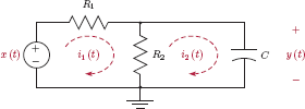
Solution: Using the two mesh currents i1 (t) and i 2 (t), and applying Kirchhoff’s voltage law (KVL) we obtain the following two equations:
We also know that the current that runs through the capacitor is proportional to the rate of change of its voltage. Therefore
Substituting Eqn. (2.20) into Eqn. (2.19) and solving for i 1 (t) yields
Finally, using Eqns. (2.20) and (2.21) in Eqn. (2.18) results in
which can be rearranged to produce the differential equation we seek:
The order of a differential equation is determined by the highest order derivative that appears in it. In Examples 2.4 and 2.5 we obtained first-order differential equations; therefore, the systems they represent are also of first order. In the next example we will work with a circuit that will yield a second-order differential equation and, consequently, a second-order system.
Example 2.6: Differential equation for RLC circuit
Find a differential equation between the input signal x(t) and the output signal y(t) to serve as a mathematical model for the series RLC circuit shown in Fig. 2.11.
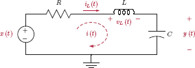
Solution: Applying KVL around the main loop we get
with x(t) and y(t) representing the input and the output signals of the system respectively. The inductor voltage is proportional to the time derivative of the current:
Similarly, realizing that the loop current i(t) is proportional to the time derivative of the capacitor voltage y(t), we can write
Differentiating both sides of Eqn. (2.25) with respect to time yields
and substituting Eqn. (2.26) into Eqn. (2.24) we obtain
Finally, substituting Eqns. (2.25) and (2.27) into Eqn. (2.23) leads to the differential equation for the RLC circuit:
Rearranging terms, we have
Thus, the RLC circuit of Fig. 2.11 leads to a second-order differential equation.
2.4 Constant-Coefficient Ordinary Differential Equations
In Section 2.2 we have discussed the properties of a class of systems known as linear and time-invariant. Linearity and time-invariance assumptions allow us to develop a robust set of methods and techniques for analyzing and designing systems. We will see in later parts of this text that, by limiting our focus to systems that are both linear and time-invariant (for which we use the acronym CTLTI), we will be able to use the convolution operation and the system function concept for the computation of the output signal.
In Examples 2.4, 2.5 and 2.6 we have explored methods of finding differential equations for several electrical circuits. In general, CTLTI systems can be modeled with ordinary differential equations that have constant coefficients. An ordinary differential equation is one that does not contain partial derivatives. The differential equation that represents a CTLTI system contains the input signal x(t), the output signal y(t) as well as simple time derivatives of the two, namely
and
A general constant-coefficient differential equation representing a CTLTI system is therefore in the form
or it can be expressed in closed summation form.
Constant-coefficient ordinary differential equation:
The order of the differential equation (and therefore the order of the system) is the larger of N and M. As an example, the differential equation given by Eqn. (2.17) for the circuit of Fig. 2.9 fits the standard form of Eqn. (2.30) with N = 1, M = 0, a1 = 1, a0 = 1/RC and b0 = 1/RC. Similarly, the differential equation given by Eqn. (2.28) for the circuit of Fig. 2.11 also conforms to the standard format of Eqn. (2.30) with N = 2, M = 0, a 2 = 1, a1 = R/L , a0 = 1/LC and b 0 = 1/LC.
In general, a constant-coefficient ordinary differential equation in the form of Eqn. (2.30) has a family of solutions. In order to find a unique solution for y(t), initial values of the output signal and its first N − 1 derivatives need to be specified at a time instant t = t0. We need to know
to find the solution for t > t0.
Example 2.7: Checking linearity and time invariance of a differential equation
Determine whether the first-order constant-coefficient differential equation
represents a CTLTI system.
Solution: In order to check the linearity of the system described by the first-order differential equation of Eqn. (2.31) we will assume that two input signals x1 (t) and x 2 (t) produce the responses y1 (t) and y2 (t) respectively. The input-output pairs must satisfy the differential equation. Therefore we have
and
Now let a new input signal be constructed as a linear combination of x1 (t) and x2 (t) in the form
where α1 and α2 are two arbitrary constants. If the system under consideration is linear, then with x3 (t) as the input signal the solution of the differential equation must be
Does y(t) = y3 (t) satisfy the differential equation when the input is equal to x(t) = x3 (t)? Using y3 (t) in the differential equation we obtain
Rearranging terms on the right side of Eqn. (2.36) we have
and substituting Eqns. (2.32) and (2.33) into Eqn. (2.37) results in
Signals x3 (t) and y3 (t) as a pair satisfy the differential equation. As a result, we may be tempted to conclude that the corresponding system is linear, however, we will take a cautious approach and investigate a bit further: Let us begin by recognizing that the differential equation we are considering is in the same form as the one obtained in Example 2.4 for the simple RC circuit. As a matter of fact it would be identical to it with a0 = b0 = 1/RC. In the simple RC circuit, the output signal is the voltage across the terminals of the capacitor. What would happen if the capacitor is initially charged to V0 volts? Would Eqn. (2.35) still be valid? Let us write Eqn. (2.35) at time t = t0:
On the other hand, because of the initial charge of the capacitor, any solution found must start with the same initial value y (t0) = V0 and continue from that point on. We must have
It is clear that Eqn. (2.39) can only be satisfied if V0 = 0, that is, if the capacitor has no initial charge. Therefore, the differential equation in Eqn. (2.31) represents a CTLTI system if and only if the initial value of the output signal is equal to zero.
Another argument to convince ourselves that a system with non-zero initial conditions cannot be linear is the following: Based on the second condition of linearity given by Eqn. (2.6), a zero input signal must produce a zero output signal (just set α1 = 0). A system with a non-zero initial state y(t0) = V0 produces a non-zero output signal even if the input signal is zero, and therefore cannot be linear.
Next we need to check the system described by the differential equation in Eqn. (2.31) for time invariance. If we replace the time variable t with (t − τ) we get
Delaying the input signal by τ causes the output signal to also be delayed by τ. Therefore, the system is time-invariant.
In Example 2.7 we verified that the first-order constant-coefficient differential equation corresponds to a CTLTI system provided that the system is initially relaxed. It is also a straightforward task to prove that the general constant-coefficient differential equation given by Eqn. (2.30) corresponds to a CTLTI system if all initial conditions are equal to zero.
Assuming that two input signals x1 (t) and x2 (t) produce the output signals y1 (t) and y2 (t) respectively, we will check and see if the input signal x3 (t) = α1x1 (t) + α2x2 (t) leads to the output signal y3 (t) = α1y1 (t) + α2y2 (t). Through repeated differentiation it can be shown that
for k = 0,...,M, and similarly,
for k = 0,...,N. Substituting Eqn. (2.41) into the left side of Eqn. (2.30) yields
Since we have assumed that [x1 (t), y1 (t)] and [x2 (t),y2 (t)] are solution pairs and therefore satisfy the differential equation, we have
Using Eqns. (2.43) and (2.44) in Eqn. (2.42) it can be shown that
where, in the last step, we have used the result found in Eqn. (2.40). As an added condition, Eqn. (2.41) must also be satisfied at t = t0 for all derivatives in the differential equation, requiring
for k = 0,...,N − 1.
The differential equation
represents a linear system provided that all initial conditions are equal to zero:
Time invariance of the corresponding system can also be proven easily by replacing T with t − τ in Eqn. (2.30):
2.5 Solving Differential Equations
One method of determining the output signal of a system in response to a specified input signal is to solve the corresponding differential equation. In later parts of this text we will study alternative methods of accomplishing the same task. The use of these alternative methods will also be linked to the solution of the differential equation to provide further insight into linear system behavior.
In this section we will present techniques for solving linear constant-coefficient differential equations. Two distinct methods will be presented; one that can only be used with a first-order differential equation, and one that can be used with any order differential equation in the standard form of Eqn. (2.30).
2.5.1 Solution of the first-order differential equation
The first-order differential equation
represents a first-order CTLTI system. This could be the differential equation of the RC circuit considered in Example 2.4 with α = 1/RC and r(t) = (1/RC)x(t). In this section we will formulate the general solution of this differential equation for a specified initial value y (t0).
Let the function f(t) be defined as
Differentiating f(t) with respect to time yields
The expression in square brackets is recognized as r(t) from Eqn. (2.48), therefore
Integrating both sides of Eqn. (2.51) over time, we obtain f(t) as
Using Eqn. (2.49)
the solution for f(t) becomes
The solution for y(t) is found through the use of this result in Eqn. (2.49):
Thus, Eqn. (2.55) represents the complete solution of the first-order differential equation in Eqn. (2.48), and is practical to use as long as the right-side function r(t) allows easy evaluation of the integral.
We may be tempted to question the significance of the solution found in Eqn. (2.55) especially since it is only applicable to a first-order differential equation and therefore a first-order system. The result we have found will be very useful for working with higher-order systems, however, when we study the state-space description of a CTLTI system in Chapter 9.
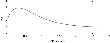
Example 2.8: Unit-step response of the simple RC circuit
Consider the simple RC circuit that was first introduced in Example 2.4. Let the element values be R = 1 Ω and C = 1/4 F. Assume the initial value of the output at time t = 0 is y (0) = 0. Determine the response of the system to an input signal in the form of a unit-step function, i.e., x(t) = u(t).
Solution: The differential equation of the circuit was obtained in Eqn. (2.17) of Example 2.4. Using the unit-step input signal specified, it can be written as
Applying Eqn. (2.57) with α = 1/RC, t0 = 0 and r(t) = (1/RC)u(t) we have
for t ≥ 0. In compact form, the result in Eqn. (2.58) is
If we now substitute the specified values of R and C into Eqn. (2.59) we obtain the output signal
which is graphed in Fig. 2.13.

Software resources:
ex_2_8.m
Example 2.9: Pulse response of the simple RC circuit
Determine the response of the RC circuit of Example 2.4 to a rectangular pulse signal
shown in Fig. 2.14. Element values for the circuit are R = 1 Ω and C = 1/4 F. The initial value of the output signal at time t = −w/ 2 is y (−w/2) = 0.

Solution: The differential equation of the circuit is obtained from Eqn. (2.17) with the substitution of specified element values and the input signal:
The solution is in the form of Eqn. (2.57) with α = 4, y (−w/2) = 0 and r(t) = 4A ∏(t/w):
The integral in this result can be evaluated using two possible ranges of the variable t.
Case 1:
In this range of t we have ∏ (t/w) = 1, and the response in Eqn. (2.61) simplifies to
which can be evaluated as
Case 2:
In this case we have ∏ (t/w) = 1 for −w/2 ≤ t ≤ w/ 2 and ∏(t/w) = 0 for t > w/ 2. The result in Eqn. (2.61) simplifies to
which leads to the response
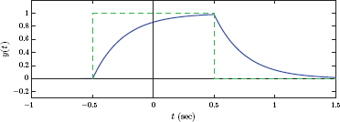
The complete response of the system can be expressed by combining the results found in Eqns. (2.62) and (2.63) as
The signal y(t) is shown in Fig. 2.15 for A = 1 and w = 1.
Software resources:
ex_2_9.m
Example 2.10: Pulse response of the simple RC circuit revisited
Rework the problem in Example 2.9 by making use of the unit-step response found in Example 2.8 along with linearity and time-invariance properties of the RC circuit.
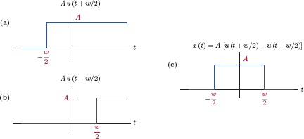
Solution: The pulse signal used as input in Example 2.9 can be expressed as the difference of two unit-step signals in the form, i.e.,
This is illustrated in Fig. 2.16.
Since the system under consideration is linear, the response to x(t) is
Furthermore, since the system is time-invariant, its responses to time-shifted unit-step functions can be found from the unit-step response that was computed in Example 2.8. It was determined that
Using the time invariance property of the system we have
and
Substituting Eqns. (2.66) and (2.67) into Eqn. (2.65) we find the pulse response of the RC circuit as
which is in agreement with the result found in Example 2.9. The steps used in the solution are illustrated in Fig. 2.17.
ex_2_10.m
Interactive Demo: rc_demo1.m
The demo “rc_demo1.m” is based on Example 2.10, Eqn. (2.65) and Fig. 2.17. The pulse response of the RC circuit is obtained from its step response using superposition. The input pulse applied to the RC circuit is expressed as the difference of two step signals, and the output signal is computed as the difference of the individual responses to step functions. Circuit parameters R and C as well as the pulse width w can be varied using slider controls.
Software resources:
rc_demo1.m
Software resources: |
See MATLAB Exercise 2.3. |
2.5.2 Solution of the general differential equation
The solution method discussed in the previous section applies to a first-order differential equation only, although, in Chapter 9, we will discuss extension of this method to higher-order differential equations through the use of state variables. In our efforts to solve the general constant-coefficient differential equation in the form given by Eqn. (2.30) we will consider two separate components of the output signal y(t) as follows:
The first term, yh (t), is the solution of the homogeneous differential equation found by ignoring the input signal, that is, by setting x(t) and all of its derivatives equal to zero in Eqn. (2.30) for all values of t:
As a mathematical function, yh (t) is the homogeneous solution of the differential equation. From the perspective of the output signal of a system, yh (t) is called the natural response of the system. As one of the components of the output signal, the homogeneous solution of the differential equation or, equivalently, the natural response of the system to which it corresponds, yh (t) depends on the structure of the system as well as the initial state of the system. It does not depend, however, on the input signal applied to the system. It is the part of the response that is produced by the system due to a release of the energy stored within the system. Recall the circuits used in Examples 2.4 through 2.6. Some circuit elements such as capacitors and inductors are capable of storing energy which could later be released under certain circumstances. If, at some point in time, a capacitor or an inductor with stored energy is given a chance to release this energy, the circuit could produce a response through this release even when there is no external input signal being applied.
When we discuss the stability property of CTLTI systems in later sections of this chapter we will see that, for a stable system, yh (t) tends to gradually disappear in time. Because of this, it is also referred to as the transient response of the system.
In contrast, the second term yp (t) in Eqn. (2.69) is part of the solution that is due to the input signal x(t) being applied to the system. It is referred to as the particular solution of the differential equation. It depends on the input signal x(t) and the internal structure of the system, but it does not depend on the initial state of the system. It is the part of the response that remains active after the homogeneous solution yh (t) gradually becomes smaller and disappears. When we study the system function concept in later chapters of this text we will link the particular solution of the differential equation to the steady-state response of the system, that is, the response to an input signal that has been applied for a long enough time for the transient terms to die out.
2.5.3 Finding the natural response of a continuous-time system
Computation of the natural response of a CTLTI system requires solving the homogeneous differential equation. Before we tackle the problem of finding the homogeneous solution for the general constant-coefficient differential equation, we will consider the first-order case. The first-order homogeneous differential equation is in the form
where α is any arbitrary constant. The homogeneous differential equation in Eqn. (2.71) has many possible solutions. In order to find a unique solution from among many, we also need to know the initial value of y(t) at some time instant t = t0. We will begin by writing Eqn. (2.71) in the alternative form
It is apparent from Eqn. (2.72) that the solution we are after is a function y(t) the time derivative of which is proportional to itself. An exponential function of time has that property, so we can make an educated guess for a solution in the form
Trying this guess1 in the homogeneous differential equation we have
which yields
By factoring out the common term cest, Eqn. (2.75) becomes
There are two ways to make the left side of Eqn. (2.76) equal zero:
- Select ce st = 0
- Select (s +α) = 0
The former choice leads to the trivial solution y(t) = 0, and is obviously not very useful. Also, as a solution it is only valid when the initial value of the output signal is y (0) = 0 as we cannot satisfy any other initial value with this solution. Therefore we must choose the latter, and use s = −α. Substituting this value of s into Eqn. (2.73) we get
where the constant c must be determined based on the desired initial value of y(t) at t = t0. We will explore this in the next two examples.
Example 2.11: Natural response of the simple RC circuit
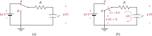
Consider again the RC circuit of Example 2.4 shown in Fig. 2.18 with the element values R = 1 Ω and C = 1/4 F. Also, let the input terminals of the circuit be connected to a battery that supplies the circuit with an input voltage of 5 V up to the time instant t = 0.

Assuming the battery has been connected to the circuit for a long time before t = 0, the capacitor voltage has remained at a steady-state value of 5 V. Let the switch be moved from position A to position B at t = 0 ensuring that x(t) = 0 for t ≥ 0. The initial value of capacitor voltage at time t = 0 is y (0) = 5 V. Find the output signal as a function of time.
Solution: Since x(t) = 0 for t > 0, the output signal is y(t) = yh (t), and we are trying to find the homogeneous solution. Substituting the specified parameter values, the homogeneous differential equation is found as
We need (s + 4) = 0, and the corresponding homogeneous solution is in the form
for t ≥ 0. The initial condition yh (0) = 5 must be satisfied. Substituting t = 0 into the homogeneous solution, we get
Using the value found for the constant c , the natural response of the circuit is
The natural response can be expressed in a more compact form through the use of the unit-step function:
This solution is shown in Fig. 2.19.
Next we will check this solution against the homogeneous differential equation to verify its validity. The first derivative of the output signal is
Using yh (t) and dyh (t)/dt in the homogeneous differential equation we have
indicating that the solution we have found is valid.
ex_2_11.m
Example 2.12: Changing the start time in Example 2.11
Rework the problem in Example 2.11 with one minor change: The initial value of the output signal is specified at the time instant t = − 0.5 seconds instead of at t = 0, and its value is y (−0.5) = 10. Physically this would correspond to using a 10 V battery instead of the 5 V battery shown in Fig. 2.18(a), and moving the switch from position A to position B at time instant t = − 0.5 seconds instead of t = 0. These differences are illustrated in Fig. 2.20.
Solution: The general form of the solution found in Example 2.11 is still valid, that is,
To satisfy yh (−0.5) = 10 we need
and therefore
The homogeneous solution is
or, using the unit step function
If the initial condition is specified at a time instant other than t = 0, then the solution we find using the procedure outlined starts at that time instant as shown in Fig. 2.21.

ex_2_12.m
We are now ready to solve the general homogeneous differential equation in the form
If we use the same initial guess
for the solution, various derivatives of y(t) will be
Through repeated differentiation it can be shown that
We need to determine which values of the parameter s would lead to valid solutions for the homogeneous differential equation. Substituting Eqn. (2.82) into Eqn. (2.80) results in
Since the term c est is independent of the summation index k , it can be factored out to yield
requiring one of the following conditions to be satisfied for y(t) = ce st to be a solution of the differential equation:
cest = 0
This leads to the trivial solution y(t) = 0 for the homogeneous equation, and is therefore not very interesting. Also, since this solution would leave us with no adjustable parameters, it cannot satisfy any non-zero initial conditions.
-
This is called the characteristic equation of the system. Values of s that are the solutions of the characteristic equation can be used in exponential functions as solutions of the homogeneous differential equation.
The characteristic equation:
The characteristic equation is found by starting with the homogeneous differential equation, and replacing the k-th derivative of the output signal y(t) with sk.
To obtain the characteristic equation, substitute:
Let us write the characteristic equation in open form:
The polynomial of order N on the left side of Eqn. (2.86) is referred to as the characteristic polynomial , and is obtained by simply replacing each derivative in the homogeneous differential equation with the corresponding power of s. Let the roots of the characteristic polynomial be s1, s2,...,sN so that Eqn. (2.86) can be written as
Using any of the roots of the characteristic polynomial, we can construct a signal
that will satisfy the homogeneous differential equation. The general solution of the homogeneous differential equation is obtained as a linear combination of all valid terms in the form of Eqn. (2.88) as
The unknown coefficients c1,c2,...,cN are determined from the initial conditions. The exponential terms eskt in the homogeneous solution given by Eqn. (2.89) are called the modes of the system. In later chapters of this text we will see that the roots sk of the characteristic polynomial of the system will be identical to the poles of the system function and to the eigenvalues of the state matrix.
Example 2.13: Time constant concept
We will again refer to the RC circuit introduced in Example 2.4 and shown in Fig. 2.9. The differential equation governing the behavior of the circuit was found in Eqn. (2.17). The characteristic equation of the system is found as
This is a first-order system, and its only mode is e−t/RC. If the initial value of the output signal is y (0) = V0, the homogeneous solution of the differential equation (or the natural response of the system) is
Let parameter τ be defined as τ = RC, and the natural response can be written as
For this type of a system with only one mode, the parameter τ is called the time constant of the system. Based on Eqn. (2.91) the time constant τ represents the amount it takes for the natural response to decay down to 1/e times or, equivalently, 36.8 percent of its initial value. This is illustrated in Fig. 2.22.
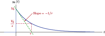
It is evident from Fig. 2.22 that the line that is tangent to yh (t) at t = 0 has a slope of −1/τ, that is,
and it intersects the time axis at t = τ. The amplitude of the output signal at t = τ is yh (τ) = V0/e.
Software resources:
ex_2_13.m
Interactive Demo: rc_demo2.m
The demo “rc_demo2.m” is based on Example 2.13, Eqn. (2.91) and Fig. 2.22. The natural response of the RC circuit is computed and graphed for a specified initial value. Circuit parameters R and C and the initial value V0 of the output signal at time t = 0 can be varied using slider controls.
- Reduce the time constant τ by reducing either R or C and observe its effect on how long it takes the natural response to become negligibly small. Can you develop a rule-of-thumb on how many time constants it takes for the natural response to become negligible?
- As the time constant is changed, observe the slope of the natural response at time t = 0. The greater the slope, the faster the natural response disappears.
Software resources:
rc_demo2.m
Example 2.14: Natural response of second-order system
The differential equation for the RLC circuit used in Example 2.6 and shown in Fig. 2.11 was given by Eqn. (2.28). Let the element values be R = 5 Ω, L = 1 H and C = 1/6F. At time t = 0, the initial inductor current is i (0) = 2 A and the initial capacitor voltage is y (0) = 1.5 V. No external input signal is applied to the circuit, therefore x(t) = 0. Determine the output voltage y(t).
Solution: Without an external input signal, the particular solution is zero, and the total solution of the differential equation includes only the homogeneous solution, that is, y(t) = yh (t). The homogeneous differential equation is
The characteristic equation of the system is
with solutions s1 = − 2and s2 = − 3. The homogeneous solution of the differential equation is in the form
for t ≥ 0. The unknown coefficients c1 and c2 need to be adjusted so that the specified initial conditions are satisfied. Evaluating yh (t) for t = 0 we obtain
Using the initial value of the inductor current we have
from which the initial value of the first derivative of the output signal can be obtained as
Differentiating the solution found in Eqn. (2.92) and imposing the initial value of dyh (t)/dt leads to
The coefficients c1 and c2 can now be determined by solving Eqns. (2.93) and (2.94) simultaneously, resulting in
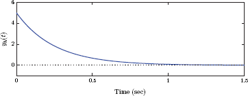
and the natural response of the system is
which is graphed in Fig. 2.23.
ex_2_14.m
In Example 2.14 the two roots of the characteristic polynomial turned out to be both real-valued and different from each other. As a result we were able to express the solution of the homogeneous equation in the standard form of Eqn. (2.89). We will now review several possible scenarios for the types of roots obtained:
Case 1: All roots are distinct and real-valued.
In this case the homogeneous solution is
as discussed above. If a real root sk is negative, the corresponding term ckeskt decays exponentially over time. Alternatively, if sk is positive, the corresponding term grows exponentially over time, and may cause the output signal to become very large without bound. Fig. 2.24 illustrates these two possibilities.
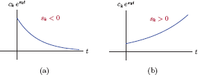
Terms corresponding to real roots of the characteristic equation: (a) sk < 0, (b) sk > 0.
Case 2: Characteristic polynomial has complex-valued roots.
Since the coefficients of the differential equation, and consequently the coefficients of the characteristic polynomial, are all real-valued, any complex roots must appear in the form of conjugate pairs. Therefore, if s1a = σ1 + jω1 is a complex root of the characteristic polynomial, then its complex conjugate must also be a root. Let the part of the homogeneous solution that is due to these two roots be
where the coefficients c1a and c1b are to be determined from the initial conditions. Continuing with the reasoning we started above, since the coefficients of the differential equation are real-valued, the homogeneous solution yh (t) must also be real. Furthermore, yh1 (t), the part of the solution that is due to the complex conjugate pair of roots we are considering, must also be real. This in turn implies that the coefficients c1a and c1b must form a complex conjugate pair as well. Let us write the two coefficients in polar complex form as
Substituting Eqn. (2.98) into Eqn. (2.97) leads to the result
- A pair of complex conjugate roots for the characteristic polynomial leads to a solution component in the form of a cosine signal multiplied by an exponential signal.
- The oscillation frequency of the cosine signal is determined by ω1, the imaginary part of the complex roots.
- The real part of the complex roots, σ1, impacts the amplitude of the solution. If σ1 < 0, then the amplitude of the cosine signal decays exponentially over time. In contrast, if σ1 > 0, the amplitude of the cosine signal grows exponentially over time. These two possibilities are illustrated in Fig. 2.25.
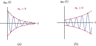
Terms corresponding to pair of complex conjugate roots of the characteristic equation: (a) σ1 < 0, (b) σ1 > 0.
Using the appropriate trigonometric identity2 it is also possible to write Eqn. (2.99) as
Case 3: Characteristic polynomial has some multiple roots.
Consider again the factored version of the characteristic equation first given by Eqn. (2.87):
What if the first two roots are equal, that is, s2 = s1? If we used the approach we have employed so far, we would have a natural response in the form
The problem with the response in Eqn. (2.101) is that we have lost one of the coefficients. For a homogeneous differential equation of order N we need to satisfy N initial conditions at some time instant t = t0, namely
To satisfy N initial conditions we need as many adjustable parameters c1,...,cN sometimes referred to as N degrees of freedom. Losing one of the coefficients creates a problem for our ability to satisfy N initial conditions. In order to gain back the coefficient we have lost, we need an additional term for the two roots at s = s1. A solution in the form
will work for this purpose. In general, a root of multiplicity r requires r terms in the homogeneous solution. If the characteristic polynomial has a factor (s − s1)r then the resulting homogeneous solution will be
Example 2.15: Natural response of second-order system revisited
Consider again the RLC circuit which was first used in Example 2.6 and shown in Fig. 2.11. At time t = 0, the initial inductor current is i (0) = 0.5 A, and the initial capacitor voltage is y (0) = 2 V. No external input signal is applied to the circuit, therefore x(t) = 0. Determine the output voltage y(t) if
- the element values are R = 2 Ω, L = 1 H and C = 1/26 F,
- the element values are R = 6 Ω, L = 1 H and C = 1/9 F.
Solution: Since no external input signal is applied to the circuit, the output signal is equal to the natural response, i.e., y(t) = yh (t), which we will obtain by solving the homogeneous differential equation. Two initial conditions are specified. The first one is that yh (0) = 2. Using the specified initial value of the inductor current we have
which leads to the initial value for the first derivative of the output signal as
Now we are ready to find the solutions for the two sets of component values given in parts (a) and (b):
Using the specified component values, the homogeneous differential equation is
and the characteristic equation is
The roots of the characteristic equation are s1 = − 1 + j5 and s2 = − 1 − j 5. The natural response is therefore in the form given by Eqn. (2.100) with σ1 = −1 and ω1 = 5 rad/s.
Now we can impose the initial conditions. The first one is straightforward:
For the specified capacitance value C = 1/26 F, the initial value of dyh (t)/dt is
To impose the specified initial value of dyh (t)/dt we will first differentiate the homogeneous solution to obtain
Evaluating this derivative at t = 0 we have
Since we previously found that d1 = 2, we need d2 = 3, and the natural response of the circuit is
for t ≥ 0. This solution is shown in Fig. 2.26(a).
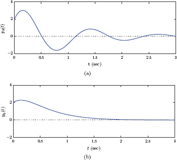
Natural responses on the RC circuit in Example 2.15 for (a) characteristic equation roots s1,2 = − 1 ± j2, and (b) characteristic equation roots s1 = s2 = − 3.
For this case the homogeneous differential equation becomes
and the characteristic equation is
Since both roots of the characteristic equation are at s1 = − 3 we will use a homogeneous solution in the form
for t ≥ 0. Imposing the initial value y (0) = 2 yields
for the first coefficient. For the specified capacitance value of C = 1/9 F the initial value of the derivative of the output signal is
To satisfy the initial condition on dyh (t)/dt we will differentiate the homogeneous solution and evaluate the result at t = 0 which yields
and leads to the result
Therefore the natural response for this case is
which is shown in Fig. 2.26(b).
Software resources:
ex_2_15a.m
ex_2_15b.m
Interactive Demo: nr_demo1
The interactive demo program nr_demo1.m illustrates different types of homogeneous solutions for a second-order continuous-time system based on the roots of the characteristic polynomial. Recall that the three possibilities were explored above, namely distinct real roots, complex conjugate roots and multiple roots.
In the demo program, the two roots can be specified using slider controls, and the corresponding natural response can be observed. If the roots are both real, then they can be controlled independently. If complex values are chosen, however, then the two roots move simultaneously to keep their complex conjugate relationship. The locations of the two roots s1 and s2 are marked on the complex plane. The differential equation, the characteristic equation and the analytical solution for the natural response are displayed and updated as the roots are moved.
Start with two real roots that are both negative, say s1 = − 1 and s2 = − 0.5. Set initial conditions as
Observe the shape of the natural response.
Gradually move s2 to the right, bringing it closer to the vertical axis. Observe the changes in the shape of the natural response. What happens when the root reaches the vertical axis, that is, when s2 = 0?
Keep moving s2 to the right until s2 = 0.3. How does the natural response change when a real root moves into the positive territory?
Set the two roots to be s1,2 = − 0.3 ± j 1.2 and observe the natural response.
Gradually increase the imaginary parts of the two roots toward ±j4 while keeping their real parts fixed at − 0.3. How does the change in the imaginary parts affect the natural response?
Gradually move the real parts of the two roots to the right while keeping the imaginary parts equal to ±j4. How does this affect the natural response? What happens when the roots cross over to the right side of the vertical axis?
Software resources:
nr_demo1.m2.5.4 Finding the forced response of a continuous-time system
In the preceding discussion we have concentrated our efforts on finding the homogeneous solution of the constant-coefficient differential equation which corresponds to the natural response yh (t) of the system under consideration when no external input signal is applied to it. To complete the solution process, we also need to determine the particular solution for a specified input signal x(t) that is applied to the system. To find the particular solution, we start with an educated guess about the form of the solution we seek, and then adjust its parameters so that the result satisfies the differential equation. The form of the particular solution should include the input signal x(t) and all of its derivatives that are linearly independent, assuming x(t) has a finite number of linearly independent derivatives. For example, if the input signal is x(t) = cos(at), we need to construct a particular solution that includes the terms cos (at) and sin(at) in the form
with parameters k1 and k2 to be determined from the differential equation. On the other hand, if the input signal is x(t) = t 3, then we need a particular solution that includes the terms t3, t2, t, and a constant term in the form
Table 2.1 lists some of the common types of input signals and the forms of particular solutions to be used for them.
Choosing a particular solution for various input signals.
Input signal |
Particular solution |
|---|---|
K (constant) |
k1 |
K eat |
k1 eat |
K cos (at) |
k1 cos (at) + k2 sin (at) |
K sin (at) |
k1 cos (at) + k2 sin (at) |
The coefficients of the particular solution are determined from the differential equation by assuming all initial conditions are equal to zero (recall that the particular solution does not depend on the initial conditions of the differential equation or the initial state of the system). The specified initial conditions of the differential equation are imposed in the subsequent step for determining the unknown coefficients of the homogeneous solution, not the particular solution.
Now we have all the tools we need to determine the forced response of the system for a specified input signal. The following is a summary of the procedure to be used:
- Write the homogeneous differential equation. Find the characteristic equation by replacing derivatives of the output signal with corresponding powers of s.
- Solve for the roots of the characteristic equation and write the homogeneous solution in the form of Eqn. (2.96). If some of the roots are complex conjugate pairs, then use the form in Eqn. (2.97) for them. If there are some multiple roots, use the procedure outlined in Eqn. (2.103) for them. Leave the homogeneous solution in parametric form with undetermined coefficients; do not attempt to compute the coefficients c1,c2, ... of the homogeneous solution yet.
- Find the form of the particular solution by either picking the appropriate form of it from Table 2.1, or by constructing it as a linear combination of the input signal and its time derivatives. (This latter approach requires that the input signal have a finite number of linearly independent derivatives.)
- Try the particular solution in the non-homogeneous differential equation and determine the coefficients k1,k2,... of the particular solution. At this point the particular solution should be uniquely determined. However, the coefficients of the homogeneous solution are still undetermined.
- Add the homogeneous solution and the particular solution together to obtain the total solution. Compute the necessary derivatives of the total solution. Impose the necessary initial conditions on the total solution and its derivatives. Solve the resulting set of equations to determine the coefficients c1,c2,... of the homogeneous solution.
These steps for finding the forced solution of a differential equation will be illustrated in the next example.
Example 2.16: Forced response of the first-order system for sinusoidal input
Consider once again the RC circuit of Fig. 2.9 with the element values of R = 1 Ω and C = 1/4 F. The initial value of the output signal is y (0) = 5. Determine the output signal in response to a sinusoidal input signal in the form
with amplitude A = 20 and radian frequency ω = 8 rad/s.
Solution: Using the specified component values, the non-homogeneous differential equation of the circuit under consideration is
and we have found in Example 2.11 that the homogeneous solution is in the form
for t ≥ 0. We will postpone the task of determining the value of the constant c until after we find the particular solution. Using Table 2.1, the form of the particular solution we seek is
Differentiating Eqn. (2.108) with respect to time yields
The particular solution yp (t) must satisfy the non-homogeneous differential equation. Substituting Eqns. (2.108) and (2.109) along with the specified input signal x(t) into the differential equation we obtain
which can be written in a more compact form as
Eqn. (2.110) must be satisfied for all values of t, therefore we must have
and
Eqns. (2.111) and (2.112) can be solved simultaneously to yield
The forced solution is obtained by adding the homogeneous solution and the particular solution together:
Let us now substitute the numerical values A = 20 and ω = 8 rad/s. The output signal becomes
Finally, we will impose the initial condition y (0) = 5 to obtain
which yields c = 4. Therefore, the complete solution is
for t ≥ 0. The solution found in Eqn. (2.114) has two fundamentally different components, and can be written in the form
The first term
represents the part of the output signal that disappears over time, that is,
It is called the transient component of the output signal. The second term
is the part of the output signal that remains after the transient term disappears. Therefore it is called the steady-state response of the system. Transient and steady-state components as well as the complete response are shown in Fig. 2.27.

Computation of the output signal of the circuit in Example 2.16: (a) transient component, (b) steady-state component, (c) the complete output signal.
Before we leave this example, one final observation is in order: The homogeneous solution for the same circuit was found in Example 2.11 as
with the input signal x(t) set equal to zero. In this example we have used a sinusoidal input signal, and the transient part of the response obtained in Eqn. (2.116) does not match the homogeneous solution for the zero-input case; the two differ by a scale factor. This justifies our decision to postpone the computation of the constant c until the very end. The initial condition is specified for the total output signal y(t) at time t = 0; therefore, we must first add the homogeneous solution and the particular solution, and only after doing that we can impose the specified value of y (0) on the solution to determine the constant c.
We will revisit this example when we study system function concepts in Chapter 7.
Software resources:
ex_2_16.m
Interactive Demo: fr_demo1
The interactive demo program fr_demo1.m is based on Example 2.16. It allows experimentation with parameters of the problem. The amplitude A is fixed at A = 20 so that the input signal is
The resistance R, the capacitance C, the radian frequency ω and the initial output value y(0) can be varied using slider controls. The effect of parameter changes on the transient response yt (t), the steady-state response yss (t) and the total forced response yt (t) + yss (t) can be observed.
- Start with the settings R = 5 Ω, C = 10 F, ω = 4 rad/s and y (0) = 0. Since the initial value of the output signal is zero, the resulting system is CTLTI. In addition, the initial value of the input signal is also zero, and therefore the output signal has no transient component. Observe the peak amplitude value of the steady-state component. Confirm that it matches with what was found in Example 2.16.
- Now gradually increase the radian frequency ω up to ω = 12 rad/s and observe the change in the peak amplitude of the steady-state component of the output. Compare with the result obtained in Eqn. (2.113).
- Set parameter values as R = 1 Ω, C = 0.3F, ω = 12 rad/s and y (0) = 4 V. The time constant is τ = RC = 0.3 s. Comment on how long it takes for the transient component of the output to become negligibly small so that the output signal reaches its steady-state behavior. (As a rule of thumb, 4 to 5 time constants are sufficient for the output signal to be considered in steady state.)
- Gradually increase the value of R to R = 3 Ω and observe the changes in the transient behavior.
Software resources:
fr_demo1.m
2.6 Block Diagram Representation of Continuous-Time Systems
Up to this point we have studied methods for analyzing continuous-time systems represented in the time domain by means of constant-coefficient ordinary differential equations. Given a system description based on a differential equation, and an input signal x(t), the output signal y(t) can be determined by solving the differential equation.
In some cases we may need to realize a continuous-time system that has a particular differential equation. Alternately, it may be desired to simulate a continuous-time system on a digital computer in an approximate sense. In problems that involve the realization or the simulation of a continuous-time system, we start with a block diagram representation of the differential equation. Once a block diagram is obtained, it may either be realized using circuits that approximate the behavior of each component of the block diagram, or simulated on a computer using code segments that simulate the behavior of each component.
In general, the problem of converting a differential equation to a block diagram has multiple solutions that are functionally equivalent even though they may look different. In this section we will present one particular technique for obtaining a block diagram from a constant-coefficient ordinary differential equation. Alternative methods of constructing block diagrams will be presented in Chapter 7 in the context of obtaining a block diagram from a system function.
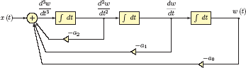
Block diagrams for continuous-time systems are constructed using three types of components, namely constant-gain amplifiers, signal adders and integrators. These components are shown in Fig. 2.28. The technique for finding a block diagram from a differential equation is best explained with an example. Consider a third-order differential equation in the form
Block diagram components for continuous-time systems: (a) constant-gain amplifier, (b) integrator, (c) signal adder.
which is in the standard form of Eqn. (2.30) with N = 3 and M = 2. The differential equation is shown in compact notation with the understanding that x(t), y(t) and all of their derivatives are functions of time. Also, for convenience, we have chosen the coefficient of the highest derivative of y(t) to be aN = 1 (which, in this case, happens to be a3). In cases where aN ≠ 1 both sides of Eqn. (2.119) can be divided by aN to satisfy this requirement.
As the first step for finding a block diagram for this differential equation, we will introduce an intermediate variable w(t). This new variable will be used in place of y(t) in the left side of the differential equation in Eqn. (2.119), and the result will be set equal to x(t) to yield
The differential equation in Eqn. (2.120) is relatively easy to implement in the form of a block diagram. Rearranging terms in Eqn. (2.120) we obtain
One possible implementation is shown in Fig. 2.29.
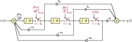
We will now show that the output signal y(t) can be expressed in terms of the intermediate variable w(t) as
This is essentially the right side of the differential equation in Eqn. (2.119) in which x(t) was replaced with w(t). Together, Eqns. (2.120) and (2.122) are equivalent to Eqn. (2.119).
The proof for Eqn. (2.122) will be given starting with the right side of Eqn. (2.119) and expressing the terms in it through the use of Eqn. (2.120). We have the following relationships:
Adding Eqns. (2.123) through (2.125) we get
proving that Eqns. (2.120) and (2.122) are indeed equivalent to Eqn. (2.119). Thus, the output y(t) can be obtained through the use of Eqn. (2.122).
Since the derivatives on the right-side of Eqn. (2.122) are readily available in the block diagram of Fig. 2.29, we will simply add the required connections to it to arrive at the completed block diagram shown in Fig. 2.30.

Even though we have used a third-order differential equation to demonstrate the process of constructing a block diagram, the extension of the technique to a general constant-coefficient differential equation is straightforward. In Fig. 2.30 the feed-forward gains of the block diagram are the right-side coefficients b0,b1,...,bM of the differential equation. Feedback gains of the block diagram are the negated left-side coefficients −a0, −a1,..., −aN−1 of the differential equation. Recall that we must have aN = 1 for this to work.
Imposing initial conditions
It is also possible to incorporate initial conditions into the block diagram. In the first step, initial values of y(t) and its first N − 1 derivatives need to be converted to corresponding initial values of w(t) and its first N − 1 derivatives. Afterwards, appropriate initial value can be imposed on the output of each integrator as shown in Fig. 2.31.
Example 2.17: Block diagram for continuous-time system
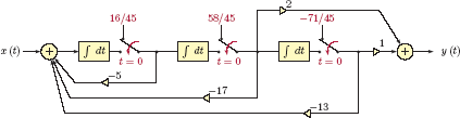
Construct a block diagram to solve the differential equation
with the input signal x(t) = cos (20πt) and subject to initial conditions
Solution: Using the intermediate variable w(t) as outlined in the preceding discussion we obtain the following pair of differential equations equivalent to the original differential equation:
Initial conditions specified in terms of the values of y, dy/dt and d2y/dt2 at time instant t = 0 need to be expressed in terms of the integrator outputs w, dw/dt and d2w/dt2 at time instant t = 0. For this purpose we will start by writing Eqn. (2.128) at time t = 0:
By differentiating both sides of Eqn. (2.128) and evaluating the result at t = 0 we obtain
Differentiating Eqn. (2.128) twice and evaluating the result at t = 0 yields
Initial value of d3w/dt3 needed in Eqn. (2.131) is obtained from Eqn. (2.127) as
Substitution of Eqn. (2.132) into Eqn. (2.131) results in
In addition we know that x (0) = 1. Solving Eqns. (2.129), (2.130) and (2.133) the initial values of integrator outputs are obtained as
The block diagram can be constructed as shown in Fig. 2.32.
2.7 Impulse Response and Convolution
In previous sections of this chapter we have explored the use of differential equations for describing the time-domain behavior of continuous-time systems, and have concluded that a CTLTI system can be completely described by means of a constant-coefficient ordinary differential equation. An alternative description of a CTLTI system can be given in terms of its impulse response h(t) which is simply the forced response of the system under consideration when the input signal is a unit impulse. This is illustrated in Fig. 2.33.
It will be shown later in this chapter that the impulse response also constitutes a complete description of a CTLTI system. Consequently, the response of such a system to any arbitrary input signal x(t) can be uniquely determined from the knowledge of its impulse response.
It should be noted that our motivation for exploring additional description forms for CTLTI systems is not due to any deficiency or shortcoming of the differential equation of the system. We know that the differential equation is sufficient for the solution of any signal-system interaction problem. The impulse response h(t) does not provide any new information or capability beyond that provided by the differential equation. What we gain through it is an alternative means of working with signal-system interaction problems which can sometimes be more convenient, and which can provide additional insight into system behavior. In the following sections we will discuss how the impulse response of a CTLTI system can be obtained from the underlying differential equation. The reverse operation is also possible, and will be discussed in later chapters.
2.7.1 Finding impulse response of a CTLTI system
When we worked on computing the forced response of a system from its differential equation, we relied on the entries in Table 2.1 to find a particular solution. First, the form of the particular solution appropriate for the type of input signal under consideration is obtained from the table. The particular solution is then tested against the differential equation, and values of any unknown coefficients are computed. Afterwards the particular solution is combined with the homogeneous solution to form the forced response of the system, and initial conditions are imposed to determine the values of any remaining coefficients.
In determining the impulse response of a system from its differential equation, we run into a roadblock: There is no entry in Table 2.1 that corresponds to an input signal in the form x(t) = δ(t). For a first-order differential equation we can use the technique outlined in Section 2.5.1 and obtain the impulse response through the use of Eqn. (2.55) with t0 = 0, y (t0) = 0 and x(τ) = δ(τ). However, this approach is not applicable to a higher-order differential equation. We will therefore take a slightly different approach in finding the impulse response of a CTLTI system:
- Use a unit-step function for the input signal, and compute the forced response of the system using the techniques introduced in previous sections. This is the unit-step response of the system.
- Differentiate the unit-step response of the system to obtain the impulse response, i.e.,
This idea relies on the fact that differentiation is a linear operator. Given that
we have
By choosing the input signal to be a unit-step function, that is, x(t) = u(t), and also recalling that du (t)/dt = δ (t), we obtain
It is important to remember that the relationship expressed by Eqn. (2.137) is only valid for a CTLTI system. This is not a serious limitation at all, since we will rarely have a reason to compute an impulse response unless the system is linear and time-invariant.
Example 2.18: Impulse response of the simple RC circuit
Determine the impulse response of the first-order RC circuit of Example 2.4, shown in Fig. 2.9, first in parametric form, and then using element values R = 1 Ω and C = 1/4 F. Assume the system is initially relaxed, that is, there is no initial energy stored in the system. (Recall that this is a necessary condition for the system to be CTLTI.)
Solution: We will solve this problem using two different methods. The differential equation for the circuit was given by Eqn. (2.17). Since we have a first-order differential equation, we can use the solution method that led to Eqn. (2.55) in Section 2.5.1. Letting α = 1/RC, t0 = 0 and y (0) = 0 we have
If the input signal is chosen to be a unit-impulse signal, then the output signal becomes the impulse response of the system. Setting x(t) = δ (t) leads to
Using the sifting property of the unit-impulse function, we obtain
Now we will obtain the same result using the more general method developed in Section 2.7.1. Recall that the unit-step response of the system was found in Example 2.8 Eqn. (2.59) as
Differentiating Eqn. (2.140) with respect to time we obtain the impulse response:
which is the same result obtained in Eqn. (2.140). With the substitution of the specified element values, the impulse response becomes
which is graphed in Fig. 2.34.

ex_2_18.m
Example 2.19: Impulse response of a second-order system
Determine the impulse response of the RLC circuit that was used in Example 2.6 and shown in Fig. 2.11. Use element values R = 2 Ω, L = 1 H and C = 1/26 F.
Solution: The homogeneous solution for the system was found in part (a) of Example 2.15 to be
We will begin by finding the unit-step response. The form of the particular solution is obtained from Table 2.1 as
Testing the particular solution with the differential equation leads to the conclusion that k1 = 1, and the complete solution is
Since we are determining the impulse response, we will naturally assume that the system is CTLTI, and is therefore initially relaxed. This requires
and
Solving Eqns. (2.141) and (2.141) yields d1 = − 1 and d2 = − 0.2. Therefore, the unit-step response of the system is
for t ≥ 0. The impulse response is found by differentiating the unit-step response with respect to time, and is
for t ≥ 0. This result is graphed in Fig. 2.35.
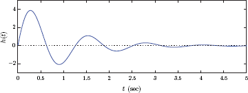
ex_2_19.m
2.7.2 Convolution operation for CTLTI systems
In Section 1.3.3 we have formulated the decomposition of an arbitrary signal into impulse functions. Specifically, we have established that a signal x(t) can be expressed through a decomposition in the form
Using Eqn. (2.144) the output signal y(t) of a system can be written in terms of its input signal x(t) as
Assuming the system under consideration is linear, we will take liberty3 to swap the order of integration and system transformation, and write the output signal as
The justification for this action can be given by considering the integral of Eqn. (2.144) as the limit case of an infinite sum as demonstrated in Chapter 1, Eqn. (1.54).
For the sake of discussion let us assume that we know the system under consideration to be linear, but not necessarily time-invariant. The response of a linear system to an impulse signal scaled by x(λ) and time-shifted by λ is
Eqn. (2.146) can therefore be written as
Using Eqn. (2.147), the response of a linear system to any arbitrary input signal x(t) can be computed, provided that we know the responses of the system to impulse signals time-shifted by all possible values. Thus, the knowledge necessary for determining the output of a linear system in response to an arbitrary signal x(t) is
While Eqn. (2.147) provides us with a viable method of determining system output y(t) for any input signal x(t), the vast amount of knowledge that we need to possess about the system makes this highly impractical.
For the result in Eqn. (2.147) to be of practical use, the prerequisite knowledge about the system must be reduced to a manageable level. Let the impulse response of the system be defined as
If, in addition to being linear, the system is also known to be time-invariant, then the response of the system to any shifted impulse signal can be derived from the knowledge of h(t) alone, that is,
consistent with the definition of time invariance given by Eqn. (2.10). Now the output signal can be written as
Eqn. (2.150) is known as the convolution integral for continuous-time signals. The output signal y(t) of a CTLTI system is obtained by convolving the input signal x(t) and the impulse response h(t) of the system. This relationship is expressed in compact notation as
where the symbol * represents the convolution operator. We will show later in this section that the convolution operator is commutative, that is, the relationship in Eqn. (2.150) can also be written in the alternative form
The roles of h(t) and x(t) can be swapped without affecting the end result.
Continuous-time convolution summary:
In computing the convolution integral it is helpful to sketch the signals. The graphical steps involved in computing the convolution of two signals x(t) and h(t) at a specific timeinstant t can be summarized as follows:
Sketch the signal x (λ) as a function of the independent variable λ. This corresponds to a simple name change on the independent variable, and the graph of the signal x (λ) appears identical to the graph of the signal x(t). (See Fig. 2.36.)
For one specific value of t, sketch the signal h (t − λ) as a function of the independent variable λ. This task can be broken down into two steps as follows:
Sketch h (−λ) as a function of λ. This step amounts to time-reversal of the signal h (λ).
In h (λ) substitute λ → λ − t. This step yields
and amounts to time-shifting h (−λ) by t.
See Fig. 2.37 for an illustration of the steps for obtaining h (t − λ).
Multiply the two signals sketched in 1 and 2 to obtain the product f (λ) = x (λ)h (t − λ).
Compute the area under the product f (λ) = x (λ)h (t − λ) by integrating it over the independent variable λ. The result is the value of the output signal at the specific time instant t.
Repeat steps 1 through 4 for all values of t that are of interest.

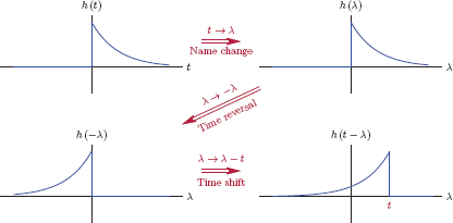
The next several examples will illustrate the details of the convolution operation for CTLTI systems.
Example 2.20: Unit-step response of RC circuit revisited
The unit-step response of the simple RC circuit was found in Example 2.8 using the direct solution method discussed in Section 2.5.1. Solve the same problem using the convolution operation.
Solution: In Example 2.18 we found the impulse response of the RC circuit to be
Based on the convolution integral of Eqn. (2.150), the two functions we need are x (λ) and h (t − λ), both as functions of λ. Fig. 2.38 shows these functions for the two cases of t ≤ 0 and of t > 0.

It is obvious that, for t ≤ 0 these two functions do not overlap anywhere, and therefore the integrand x (λ)h (t − λ) of the convolution integral is zero for all values of λ. Thus, an easy conclusion is
If t > 0, the two functions x (λ) and h (t − λ) overlap for values of λ in the interval (0,t). In this interval, we have x (λ) = 1 and . Therefore, the output signal is
Using a unit-step function to account for both segments of the solution found, the general solution valid for all t can be written as
which agrees with the result found in Example 2.8 by solving the differential equation directly.
Interactive Demo: conv_demo1.m
The demo program “conv_demo1.m” is based on Example 2.20, and allows visualization of the convolution operation. Signals x (λ), h (t − λ) and the product [x (λ)h (t − λ)] are graphed on the left side of the demo screen. The time variable can be advanced by means of a slider control. As the time t is varied, graphs for the factor h (t − λ) and the integrand [x (λ)h (t − λ)] are updated. The area under the integrand [x (λ)h (t − λ)] is shaded to correspond to the result of the integral for that particular value of t.
Software resources:
conv_demo1.m
Example 2.21: Pulse response of RC circuit revisited
Using convolution, determine the response of the simple RC circuit of Example 2.4 to a unit-pulse input signal x(t) = Λ(t).
Solution: As in the previous example, it will be useful to sketch the functions involved in the convolution integral, namely x (λ) and h (t − λ). In doing so, we will consider three distinctly different possibilities for the time variable t as shown in Fig. 2.39.
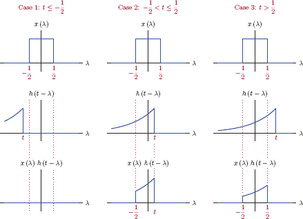
The convolution integral will be evaluated separately for each of the three cases. It is suggested that the reader follow the development below while using the interactive demo program “conv_demo2.m” to observe the overlaps of x (λ) and h (t − λ) in each of the three cases.
There is no overlap between the two functions in this case, therefore their product equals zero for all values of λ. As a result, the output signal is
Case 2:
For this case, the two functions overlap in the range . Setting integration limits accordingly, we can compute the output signal as
Case 3:
For this case, the overlap of the two functions will occur in the range . Setting integration limits to the endpoints of this new range, we have
We have computed the output signal in each of the three distinct time intervals we have identified, mainly before the start of the pulse, during the pulse, and after the end of the pulse. Putting these three partial solutions together, the complete solution for the output signal is obtained as
and is shown in Fig. 2.40.
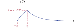
It is easy to see that the output signal found in Eqn. (2.157) becomes identical to the result obtained in Eqn. (2.64) of Example 2.9 if we set A = 1, w = 1, R = 1 Ω and C = 1/4F.
ex_2_21.m
Interactive Demo: conv_demo2.m
The demo program “conv_demo2.m” is based on Example 2.21, Fig. 2.39 and Fig. 2.40. It allows visualization of the convolution operation. The graphical user interface is similar to that of “conv_demo1.m” except it is adapted to use the signals of Example 2.21.
Software resources:
conv_demo2.m
Example 2.22: A more involved convolution problem
Consider a system with the impulse response
Let the input signal applied to this system be
Determine the output signal y(t) using convolution.
Solution: The functions x (λ) and h (t − λ) involved in the convolution integral are shown in Fig. 2.41.
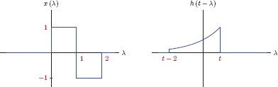
For this problem we will need to distinguish between six different regions for the time variable t as shown in Fig. 2.42. The demo program “conv_demo3.m” can be used along with the solution outlined below to observe the overlapped regions in time.

Case 1: t ≤ 0
The functions x (λ) and h (t − λ) do not overlap for t ≤ 0, and therefore their product equals zero for all values of λ. As a result, the output signal is
In this case the two functions overlap for the range 0 < λ ≤ t. The output signal is
Case 3: 1 < t ≤ 2
In this case the two functions overlap for the range 0 < λ ≤ t. In the interval 0 < λ ≤ 1 we have x (λ) = 1, and the resulting integrand is positive. On the other hand, in the interval 1 < λ ≤ t we have x (λ) = − 1, and the integrand is negative. As a result, two integrals will be needed for the solution:
Case 4: 2 < t ≤ 3
In this case the overlap region is t − 2 < λ ≤ 2. Furthermore, the left edge of h (t − λ) is in the interval 0 < t − 2 ≤ 1. In the interval t − 2 < λ ≤ 1 the input signal is x (λ) = 1, and the resulting integrand [x (λ)h (t − λ)] is positive. In the remainder of the overlap interval, that is, for 1 < λ ≤ 2 we have x (λ) = −1, and the integrand is negative. Again, two integrals will be formed:
Case 5: 3 < t ≤ 4
In this case the overlap region is t − 2 < λ ≤ 2. The left edge of h (t − λ) is in the interval 1 < t − 2 ≤ 2. The output signal is
Case 6: t > 4
The functions x (λ) and h (t − λ) do not overlap for t> 4, and therefore the output signal is
The complete output signal is graphed in Fig. 2.43 by combining the results found for all six regions of time.
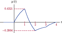
ex_2_22.m
Interactive Demo: conv_demo3.m
The demo program “conv_demo3.m” is based on Example 2.22. It facilitates visualization of the overlapping regions between the functions x (λ) and h (t − λ) as the time variable t is varied. The graphical user interface is similar to the user interfaces of “conv_demo1.m” and “conv_demo2.m”.
Software resources:
conv_demo3.m
We have stated in Eqn. (2.152) that the convolution operator is commutative. The proof is straightforward, and will now be given.
Let us apply the variable change t − λ = γ to the integral in Eqn. (2.150), and write it as
where we have also used the two consequences of the variable change employed, namely
- dλ = −dλ
- λ → ± ∞ means γ → ∓∞
Swapping the integration limits in Eqn. (2.158) and negating the integral to compensate for it, the output signal can now be written as
thus proving the commutative property of the convolution operator.
The following example will illustrate the use of the alternative form of the convolution integral based on the commutative property.
Example 2.23: Using alternative form of convolution
Find the unit-step response of the RC circuit with impulse response
using the alternative form of the convolution integral given by Eqn. (2.159).
Solution: Using the convolution integral of Eqn. (2.159), the two functions we need are h (γ) and x (t − γ), both as functions of γ. Fig. 2.44 shows these functions for the two cases of t ≤ 0 and of t > 0. For t ≤ 0 these two functions do not overlap anywhere, and therefore the integrand [h (γ)x (t − γ)] of the convolution integral is zero for all values of γ. We therefore conclude that

For values of t > 0, the two functions h (γ) and x (t − γ) overlap for values of γ in the interval (0,t). In this interval, we have x (t − γ) = 1 and . Therefore, the output signal is
Using a unit-step function to account for both segments of the solution found, the general solution valid for all t is
which agrees with the result found in Example 2.20.
Interactive Demo: conv_demo4.m
The demo program “conv_demo4.m” is based on Example 2.23. It facilitates visualization of the overlapping regions between the functions h (γ) and x (t − γ) as the time variable t is varied. The graphical user interface is identical to the user interface of “conv_demo1.m”.
Software resources:
conv_demo4.m
2.8 Causality in Continuous-Time Systems
Causality is an important feature of physically realizable systems. A system is said to be causal if the current value of the output signal depends only on current and past values of the input signal, but not on its future values. For example, a continuous-time system with input-output relationship
is causal since the output signal can be computed based on current and past values of the input signal. Conversely, the system given by
is non-causal since the computation of the output signal requires anticipation of a future value of the input signal.
Can a non-causal system be realized?
The answer depends on what type of realization we seek. Consider the system represented by Eqn. (2.161). For the sake of discussion, suppose that the signal x(t) is the output of a microphone in a recording studio where a live band is playing. The signal is delayed by 0.01 seconds and 0.02 seconds in two separate systems, and the outputs of these delay systems are added to the original signal x(t) to produce the signal y(t) in real time, that is, while the input signal is being played. This type of signal processing is called real-time processing, and is illustrated in Fig. 2.45.
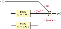
Now consider the system in Eqn. (2.162). Clearly, this system cannot be realized for real-time processing since the value x (t + 0.01) is not available at the time instant t when the output is computed. If we must realize this system (some non-causal systems may have desired properties in other respects) then we must realize it in post processing mode. The signals x(t), x (t − 0.01), and x (t + 0.01) are each recorded. The output signal is then computed from these recordings after the fact, e.g., after the band finishes playing the song. Another way to look at this type of processing is to consider a new signal w(t) defined as
and write the system description in terms of the new, delayed, output signal w(t) in the form
The signal w(t) can be computed in real time, and we can listen to it while the band is playing. However, it represents a delayed version of the actual output signal y(t) that is of interest to us. In essence we are doing post processing. Some non-causal systems can be made causal through the addition of delays as we have done in Eqn. (2.163). However, we will see that this is not always possible.
For CTLTI systems the causality property can be related to the impulse response of the system. Recall that the output signal y(t) of the system is equal to the convolution of its input signal x(t) and its impulse response h(t). We will use the alternative form of the convolution integral given by
For the system under consideration to be causal, computation of y(t) should not require any future values of the input signal. Consequently, the term x (t − λ) in the integral should not contain references to any future values. We need
and equivalently λ ≥ 0. Thus, the integrand in Eqn. (2.166) should not have any non-zero values for λ < 0. This in turn requires that the impulse response of the system be equal to zero for all negative values of its argument, i.e.,
This result intuitively makes sense. The impulse response of a causal CTLTI system cannot possibly start before t = 0 since doing so would require the system to anticipate the impulse to occur at t = 0. Using Eqn. (2.167), the convolution relationship in Eqn. (2.165) can be written in the right-sided form
2.9 Stability in Continuous-Time Systems
A system is said to be stable in the bounded-input bounded-output (BIBO) sense if any bounded input signal is guaranteed to produce a bounded output signal.
An input signal x(t) is said to be bounded if an upper bound Bx exists such that
for all values of t. It doesn’t matter how large the upper bound Bx may be, as long as it is finite. For the system to be stable a finite upper bound By must exist for the output signal in response to any input signal bounded as described by Eqn. (2.169).
For stability of a continuous-time system:
If the system under consideration is CTLTI, then we would like to relate the stability condition given by Eqn. (2.170) to the impulse response of the system as well as its differential equation. Derivation of the necessary condition follows:
The output signal of a CTLTI system is found from its input signal and impulse response through the use of the convolution integral
The absolute value of the output signal is
Absolute value of an integral is less than or equal to the integral of the absolute value of the integrand, so we can write the inequality
The integrand in Eqn. (2.173) can be expressed as
and the inequality in Eqn. (2.173) becomes
Since x (t − τ) < Bx we can write Eqn. (2.175) as
or, equivalently
Eqn. (2.177) implies that we need
For a CTLTI system to be stable, its impulse response must be absolute integrable.
Example 2.24: Stability of a first-order continuous-time system
Evaluate the stability of the first-order CTLTI system described by the differential equation
where a is a real-valued constant.
Solution: The impulse response of the system in question is
as can be easily verified through the use of Eqn. (2.55) with r(t) = δ (t), t0 = 0 and y (0) = 0. (We take the initial value to be zero since the system is specified to be CTLTI.) Now we can check to see if the requirement given by Eqn. (2.178) is satisfied.
Thus the system is stable if a > 0. (Verify that the integral in Eqn. (2.179) cannot be evaluated if a ≤ 0.) It is also interesting to recognize that the characteristic equation that corresponds to the differential equation of the system is
and its only solution is at s1 = −a.
The stability of a CTLTI system can also be associated with the modes of the differential equation that governs the behavior of the system. In Example 2.24 the system proved to be stable for a > 0 which meant that the only root of the characteristic polynomial had to be negative. Furthermore, we have seen in Section 2.5.3 that the locations of the roots of the characteristic polynomial control the type of the transient behavior of the system. In the case of real roots, a negative real root leads to a decaying exponential signal while a positive real root produces a growing exponential signal. In the case of a pair of complex conjugate roots, if the real part of the pair is negative, the resulting signal is oscillatory with exponentially decaying amplitude. If the real part of the conjugate pair is positive, then the oscillatory response has a growing amplitude. Summarizing both cases we can conclude that, for a causal system, characteristic polynomial roots in the left half of the complex plane are associated with stable behavior, and those in the right half of the complex plane are associated with unstable behavior. For a causal CTLTI system to be stable, all roots of the characteristic polynomial must be in the left half of the complex plane.
A side note: In describing the associations between the roots of the characteristic polynomial and stability, we referred to a causal CTLTI system. If we were to consider an anti-causal system, the impulse response of which proceeds in the negative direction toward t → −∞, then the associations described above would have to be reversed. In that case roots in the right half of the complex plane would lead to stable behavior.
Why is stability important for a CTLTI system?
An unstable CTLTI system is capable of producing an unbounded output signal in response to at least some bounded input signals. What is the practical significance of this? Consider a battery-operated amplifier circuit that may be unstable due to a design flaw. We certainly don’t expect the voltages in a battery-operated device to be infinitely large, and it does not happen. What may happen is that the output voltage may go up to the maximum level it can physically attain (probably close to the power supply voltage) and stay there, causing circuit components to saturate, and causing the system to cease its useful linear operation. Another example would be an electromechanical system such as an electric motor. If it is unstable as a system, its speeds may reach levels that are too high for its normal operation, and cause physical damage to the motor.
2.10 Approximate Numerical Solution of a Differential Equation
For a system modeled by means of a differential equation, the output signal can be determined by solving the differential equation with the specified input signal and initial conditions. In Section 2.5 we have explored time-domain methods for solving linear differential equations with constant coefficients. Transform-domain methods for accomplishing the same task will be presented in Chapter 7.
Sometimes we may run into differential equations for which analytical solutions may be difficult or impossible to obtain. The differential equation may have nonlinear terms, or the analytical definition of the input signal applied to the system may not be simple or practical enough for obtaining an analytical solution. In those cases, we may have to rely on approximate step-by-step solutions that are obtained on a computer by the use of an iterative numerical algorithm. A number of numerical algorithms for finding approximate solutions to differential equations are documented in the literature, ranging from very simple to very sophisticated. A thorough review of these algorithms is also well beyond the scope of this text, and can be found in a number of excellent textbooks on numerical analysis. In this section we will briefly discuss the simplest of the numerical solution methods, the Euler method, which works reasonably well for our purposes as long as some basic precautions are taken.
Consider the RC circuit that was analyzed in Examples 2.8 and 2.9 using analytical solution techniques. The first-order differential equation that governs the operation of the circuit is
where x(t) and y(t) represent the input and the output signals respectively. The first step will be to rearrange the terms of the differential equation so that the derivative of the output signal is left by itself on the left side of the equal sign:
Eqn. (2.181) is in the general form
where g (...) represents some function of t and y(t). For this particular circuit we have
We know from basic calculus that one way of approximating a derivative is through the use of finite differences. At the time instant t = t0, the derivative on the left side of Eqn.
provided that the time step T is sufficiently small. This is illustrated in Fig. 2.46. The slope of the tangent passing through the point [t0,y (t0)] represents the true value of the derivative dy (t)/dt at t = t0. The slope of the chord passing through the points [t0,y (t0)] and [t0 + T, y (t0 + T)] is the approximate value of the same.
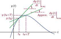
Substituting Eqn. (2.184) into Eqn. (2.182) and rearranging the terms we obtain
which gives us the iteration formula for the Euler method. The solution starts with a known initial value of the output signal at the time instant t = t0, typically t = 0. Suppose y (0) is given. We use it to approximate y (T) as
For the RC circuit example, Eqn. (2.186) becomes
Having obtained an approximate value for y (T), we can use it to approximate the solution at the time instant t = 2T as
The knowledge of an approximate value for y (2T) can then be used for finding an approximate value for y (3T) as
and so on. For this approximation technique to work in a reasonably accurate manner, the step size T needs to be chosen to be small enough. As far as the system is concerned, a good rule of thumb is for the step size T to be 10 percent of the time constant or smaller. In addition, time variations of the input signal must also be considered in selecting the step size. The Euler method may suffer from numerical instability problems if the step size T is not chosen small enough. A variant known as the backward Euler method improves the stability of the solution. The discussion of sampling in Chapter 6 will further clarify this issue.
Although the Euler method as presented in this section only applies to a first-order differential equation, we will be able to generalize it to apply to higher-order systems when we discuss state-space models in Chapter 9.
MATLAB Exercises 2.4 and 2.5 provide examples of finding numerical solutions in MATLAB using the Euler method or the more sophisticated methods MATLAB implements.
Software resources: |
See MATLAB Exercises 2.4 and 2.5. |
2.11 Further Reading
[1] S.C. Chapra.Applied Numerical Methods with MATLAB for Engineers and Scientists. McGraw-Hill, 2008.
[2] S.C. Chapra and R.P. Canale.Numerical Methods for Engineers. McGraw-Hill, 2010.
[3] T.L. Harman, J.B. Dabney, and N. Richert.Advanced Engineering Mathematics Using MATLAB V.4. PWS BookWare Companion Series. PWS Publishing Company, 1997.
[4] P.V. O’Neil.Advanced Engineering Mathematics. Cengage Learning, 2011.
[5] Frank L. Severance.System Modeling and Simulation: An Introduction. John Wiley and Sons, 2001.
[6] C.R. Wylie and L.C. Barrett.Advanced Engineering Mathematics. McGraw-Hill, 1995.
MATLAB Exercises
MATLAB Exercise 2.1: Testing linearity of continuous-time systems
In Example 2.1 we have checked four different systems for linearity. In each case we started with two arbitrary signals x1 (t) and x2 (t). We have formulated the response of each system to the combined signal
with arbitrary constants α1 and α2, and determined if the response to the combined signal matched the expected response
for a linear system. In this exercise, we will simulate the four systems considered in Example 2.1, and test them using signals generated in MATLAB.
Let us begin by creating a vector “t” of time instants, and generating vectors “x1”and “x2” to correspond to two test signals x1 (t) and x2 (t) with the following commands:
>> t = [0:0.01:5];
>> x1 = cos (2*pi*5*t);
>> x2 = exp (-0.5* t);
Let α1 = 2 and α2 = 1.25. The vector “x” will hold amplitudes of the combined input signal x(t) = α1x1 (t)+α2x2 (t) at the time instants listed in vector “t”. To compute and graph x(t) type the following set of commands:
>> alpha1 = 2;
>> alpha2 = 1.25;
>> x = alpha1*x1+alpha2*x2;
>> plot (t,x);
We are now ready to simulate the system under consideration. One method for doing this is to develop a MATLAB function for each system. For example, the system in part (a) of Example 2.1 can be simulated using the function sys_a(..) defined with the following code:
1 function y = sys_a(x)
2 y = 5* x;
These two lines must be placed into a file named “sys a.m” and saved at a location visible to MATLAB. An alternative is to use anonymous functions that were introduced in MATLAB Exercise 1.3. An anonymous function for the system in part (a) of Example 2.1 can be entered by typing
>> sys_a = @(x)5*x;
directly into the command window. This is the preferred approach in situations where the function in question may be needed only briefly, and we may not want to save it to disk. Once the function is defined, the response expected from a linear system and the actual response of our system can be obtained by typing the following lines:
>> y1 = sys_a x1);
>> y2 = sys_a(x2);
>> y_exp = alpha1*y1+alpha2*y2;
>> y_act = sys_a(x);
The vector “y exp” holds the response expected from a linear system, and the vector “y act” holds the output signal produced by the system in response to the combined input signal in vector “x”.
The MATLAB script listed below represents a complete program that tests the system in part (a) of Example 2.1 for linearity.
1 % Script : matex_2_1.m
2 %
3 t = [0:0.01:4]; % Create a time vector.
4 x1 = cos (2* pi*5* t); % Test signal 1.
5 x2 = exp (-0.5* t); % Test signal 2.
6 alpha1 = 2; % Set parameters alpha1
7 alpha2 = 1.25; % and alpha2.
8 x = alpha1*x1+alpha2*x2; % Combined signal.
9 % Define anonymous functions for the systems in Example 2-1.
10 sys_a = @(x) 5*x;
11 sys_b = @(x) 5*x+3;
12 sys_c = @(x) 3*x.*x;
13 sys_d = @(x) cos(x);
14 % Test the system in part (a) of Example 2-1.
15 y1 = sys_a (x1);
16 y2 = sys_a (x2);
17 y_exp = alpha1*y1+alpha2*y2; % Expected response for a linear system.
18 y_act = sys_a(x); % Actual response.
19 clf; % Clear figure.
20 subplot (1,2,1);
21 plot(t,y_exp); % Graph expected response.
22 title ('y_{exp} = alpha_1 y_1 + alpha_2 y_2 ')
23 xlabel ('t (sec)'),
24 ylabel ('Amplitude '),
25 subplot (1,2,2);
26 plot(t,y_act); % Graph actual response.
27 title('y_{act} = Sys_a { alpha_1 x_1 + alpha_2 x_2 }')
28 xlabel ('t (sec)'),
29 ylabel ('Amplitude '),
The graph produced by the script is shown in Fig. 2.47.
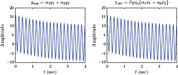
The two signals seem to be identical, supporting our earlier conclusion that the system in part (a) is linear. A word of caution is in order here: For a system to be linear, superposition principle must hold for any two signals x1 (t) and x2 (t) and not just the two signals we generated above. If we only had the graphs in Fig. 2.47 without our earlier analysis of Example 2.1, we would not be able to claim that the system is linear; the best we could do would be to say that the system may be linear. Nonlinearity of a system is easier to prove; we only need to show one case where superposition fails.
The systems in parts (b) through (d) of Example 2.1 can be simulated by editing the code above and changing the anonymous function used for the system.
Software resources:
matex_2_1.m
MATLAB Exercise 2.2: Testing time invariance of continuous-time systems
In Example 2.2 we have checked three systems for time invariance. In each case an arbitrary test signal was used with the system in its original form x(t) and in time-shifted form x (t − τ). If the system under consideration is time-invariant we need
where y(t) is the response to the original signal x(t).
In this exercise, we will simulate the three systems considered in Example 2.2, and test them using signals generated in MATLAB. Recall that, in MATLAB Exercise 2.1, anonymous functions were used for simulating the systems, and MATLAB vectors were used for simulating of the input signals. For the purpose of this exercise we will find it more convenient to use an anonymous function for the input signal as well, since time shifts are easier to represent with functions rather than vectors.
We will begin by creating a vector “t” of time instants, and developing an anonymous function “x” for the test signal x(t) with the following commands:
>> t = [0:0.01:10];
>> x = @(t) exp(-0.5*t).*(t >=0);
>> plot (t,x(t),t,x(t -2));
We are now ready to simulate the system under consideration. For the sake of discussion, let’s pick the system in part (c) of Example 2.2 and express it with an anonymous function as
>> sys_c = @(x) 3*cos(t).*x;
directly into the command window. We are now ready to compute the responses of the system to the signals x(t) and x (t − 2) as
>> y1 = sys_c (x(t));
>> y2 = sys_c (x(t-2));
Vectors “y1” and “y2” are vectors that hold the responses of the system under consideration. The two responses can be graphed on the same coordinate system with the statement
>> plot(t,y1,’b -’,t,y2,’r:’);
The MATLAB script listed below represents a complete program that tests the system in part (c) of Example 2.2 for time-invariance.
1 % Script matex_2_2.m
2 %
3 t = [0:0.01:10]; % Create a time vector.
4 x = @(t) exp(-0.5*t).*(t>=0); % Anonymous function for test signal.
5 % Define anonymous functions for the systems in Example 2-2.
6 sys_a = @(x) 5*x;
7 sys_b = @(x) 3*cos(x);
8 sys_c = @(x) 3*cos(t).*x;
9 % Test the system in part (c) of Example 2-2.
10 y1 = sys_c (x(t));
11 y2 = sys_c (x(t -2));
12 clf; % Clear figure.
13 plot(t,y1,'b-',t,y2 ,'r:'), % Graph the two responses.
14 title ('Responses to x(t) and x(t-2)')
15 xlabel ('t (sec)'),
16 ylabel ('Amplitude '),
17 legend ('Sys {x(t)} ','Sys {x(t-2)} '),
The graph produced by the script is shown in Fig. 2.48.
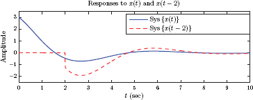
The two signals seem to be different in shape, supporting our earlier conclusion that the system in part (c) is not time-invariant. The systems in parts (a) and (b) of Example 2.2 can be simulated by editing the code above and changing the anonymous function used for the system.
Software resources:
matex_2_2.m
MATLAB Exercise 2.3: Using linearity to determine the response of the RC circuit
Refer to Examples 2.8, 2.9 and 2.10. In Example 2.8 the unit-step response of the simple RC circuit was determined by solving the governing differential equation. The circuit was assumed to be initially relaxed, resulting in y (0) = 0. In Example 2.9 we have determined the response of the same circuit to a pulse signal, again by solving the differential equation. Example 2.10 explored an alternative approach to finding the response to the pulse signal; namely using the response to a unit-step and the superposition principle. (Superposition could be used since the circuit is initially relaxed and therefore linear and time-invariant.)
In this exercise we will explore this concept using MATLAB. The response of the circuit to a unit-step signal was found in Example 2.8 to be
which can be expressed by means of an anonymous function as
yu = @(t)(1-exp(-4*t)).*(t>=0);
The script listed below uses the unit-step response for determining and graphing the response of the system to the pulse signal
1 % Script : matex_2_3a.m
2 %
3 % Anonymous function for unit - step response.
4 yu = @(t) (1-exp(-4* t)).*(t>=0);
5 t = [-5:0.01:5]; % Vector of time instants.
6 y1 = yu(t+0.5)-yu(t-0.5); % Compute response to x1(t).
7 plot (t, y1);
This idea can be extended to input signals with higher complexity. Consider the signal
which is shown in Fig. 2.49.
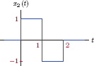
1 % Script : matex_2_3b.m
2 %
3 % Anonymous function for unit-step response.
4 yu = @(t) (1-exp(-4*t)).*(t>=0);
5 t = [-5:0.01:5]; % Vector of time instants.
6 y2 = yu(t)-2*yu(t-1)+yu(t-2); % Compute response to x2(t)].
7 plot(t,y2);
Software resources:
matex_2_3a.m
matex_2_3b.m
MATLAB Exercise 2.4: Numerical solution of the RC circuit using Euler method
In this exercise we will use the Euler method to find an approximate numerical solution for the RC circuit problem of Example 2.8, and compare it to the exact solution that was found. The RC circuit and the input signal are shown in Fig. 2.50.
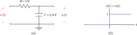
For the specified input signal, the differential equation of the circuit is
With the circuit initially relaxed, that is, with y(0) = 0, the exact solution for the output signal was found to be
In order to use the Euler method for approximate solution, we will write the differential equation in the form
with the right-side function given by
The Euler method approximation to the solution is based on the iteration formula
The MATLAB script given below computes and graphs exact and approximate solutions, using a step size of Ts = 0.1 s. In addition, the percent error of the approximate solution is computed as
and graphed for k = 1, 2, . . . , 10 to span a time interval of 1 s.
1 % Script : matex_2_4.m
2 %
3 Ts = 0.1; % Time increment
4 t = [0:Ts:1]; % Vector of time instants
5 % Compute the exact solution.
6 y = 1-exp(-4*t); % Eqn .(2.186)
7 % Compute the approximate solution using Euler method.
8 yhat = zeros (size(t));
9 yhat (1) = 0; % Initial value.
10 for k = 1: length(yhat)-1,
11 g = -4* yhat(k)+4; % Eqn .(2.188)
12 yhat(k+1) = yhat(k)+Ts*g; % Eqn .(2.189)
13 end;
14 % Graph exact and approximate solutions.
15 clf;
16 subplot (211);
17 plot(t,y,'-',t,yhat ,'ro'), grid;
18 title('Exact and approximate solutions for RC circuit '),
19 xlabel ('Time (sec)'),
20 ylabel ('Amplitude '),
21 legend ('Exact solution ','Approximate solution ' ,...
22 'Location ','SouthEast '),
23 % Compute and graph the percent approximation error.
24 err_pct = (yhat -y)./y*100;
25 subplot (212);
26 plot(t(2: length (t)), err_pct (2: length (t)), 'ro'), grid
27 title('Percent approximation error '),
28 xlabel ('Time (sec)'),
29 ylabel ('Error (%) '),
The loop that runs from line 10 to 13 of the code computes the approximate solution step by step. The graphs produced by the MATLAB script above are given in Fig. 2.51. The largest approximation error seems to be around 21 percent, and it goes down in time as the output signal settles close to its final value.

Actual and approximate solutions for the RC circuit and the percent error for Δt = 0.1 s.
The time step that we used in the code above was Ts = 0.1 seconds which is 40 percent of the time constant of τ = 0.25 s. For better accuracy a smaller time step is needed. Euler method is a first-order approximation method, and is the simplest of all numerical methods for solving differential equations. Fig. 2.52 shows the results obtained with the same script, by simply changing the step size to Ts = 0.02 seconds or 8 percent of the time constant. In this case, the largest error between the exact and approximate solutions is on the order of 4 percent.
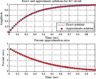
Actual and approximate solutions for the RC circuit and the percent error for Δt = 0.02 s.
Another way to reduce the approximation error is to use a more sophisticated higher-order approximation method as we will see in the next exercise.
Software resources:
matex_2_4.m
MATLAB Exercise 2.5: Improved numerical solution of the RC circuit
For numerical solution of differential equations MATLAB has a number of functions that are based on more sophisticated algorithms than the Euler method we have used in MATLAB Exercise 2.4. In this exercise we will use one of those functions, namely the function ode45(..). The function ode45(..) uses the 4-th order Runge-Kutta technique, a higher-order method than the Euler method of the previous example. For a given step size, approximation errors for the 4-th order Runge-Kutta technique are generally smaller than those encountered with the Euler method.
Before we can use the function ode45(..), we need to write a function to compute the right side g (t, y (t)) of the differential equation. The code for such a function rc1(..) is given below:
1 function ydot = rc1(t,y)
2 ydot = -4*y+4;
3 end
The function rc1(..) takes two arguments, t and y, and returns the corresponding value of g (t, y (t)). It is used by the function ode45(..) in computing the approximate solution. The script listed below computes an approximate solution in the time interval 0 ≤ t ≤ 1 s using a time step of T = 0.1 s, and compares it to the exact solution.
1 % Script : matex_2_5a.m
2 %
3 t = [0:0.1:1]; % Vector of time instants
4 % Compute the exact solution.
5 y = 1- exp (-4* t); % Eqn.(2.187)
6 % Compute the approximate solution using ode45 ().
7 [t, yhat] = ode45 (@rc1,t,0);
8 % Graph exact and approximate solutions.
9 clf ;
10 subplot (211);
11 plot (t,y, '-',t, yhat,'ro '), grid ;
12 title ('Exact and approximate solutions for RC circuit '),
13 xlabel ('Time (sec) '),
14 ylabel (' Amplitude '),
15 legend (' Exact solution ',' Approximate solution ',...
16 ' Location ',' SouthEast '),
17 % Compute and graph the percent approximation error.
18 err_pct = (yhat -y ')./y '*100;
19 subplot (212);
20 plot (t (2: max (size (t))), err_pct (2: max (size (t))), 'ro '), grid
21 title ('Percent approximation error '),
22 xlabel ('Time (sec) '),
23 ylabel (' Percent error '),
Graphs produced by the script matex_2_5a.m are shown in Fig. 2.53. Even though the step size is quite large, the accuracy of the solution obtained is much better than that obtained in the previous exercise (compare Fig. 2.53 to Fig. 2.51).

Actual and approximate solutions for the RC circuit and the percent error with the ode45(..) function.
If the right-side function g (t, y (t)) is simple enough to be expressed on one line, an anonymous function can be used in place of “rc1.m”. The script listed below uses an anonymous function “rc2” to solve the same problem.
1 % Script : matex_2_5b.m
2 %
3 t = [0:0.1:1]; % Vector of time instants
4 % Compute the exact solution.
5 y = 1-exp (-4* t); % Eqn.(2.187)
6 % Compute the approximate solution using ode45 ().
7 rc2 = @(t, y) -4*y+4;
8 [t, yhat] = ode45 (rc2,t,0);
9 % Graph exact and approximate solutions.
10 clf;
11 subplot (211);
12 plot (t,y,'-',t,yhat,'ro '), grid ;
13 title (' Exact and approximate solutions for RC circuit '),
14 xlabel ('Time (sec)'),
15 ylabel (' Amplitude '),
16 legend ('Exact solution ',' Approximate solution ',...
17 ' Location ',' SouthEast '),
18 % Compute and graph the percent approximation error.
19 err_pct = (yhat -y ')./y '*100;
20 subplot (212);
21 plot (t (2: max (size (t))), err_pct (2: max (size (t))), 'ro '), grid
22 title (' Percent approximation error '),
23 xlabel ('Time (sec)'),
24 ylabel ('Percent error '),
Software resources:
matex_2_5a.m
rc1.m
matex_2_5b.m
Problems
2.1. A number of systems are specified below in terms of their input-output relationships. For each case, determine if the system is linear and/or time-invariant.
- y(t) = |x (t)| + x(t)
- y(t) = tx (t)
- y(t) = e−t x (t)
2.2. Consider the cascade combination of two systems shown in Fig. P.2.2(a).
Let the input-output relationships of the two subsystems be given as
Write the relationship between x(t) and y(t).
- Let the order of the two subsystems be changed as shown in Fig. P.2.2(b). Write the relationship between x(t) and . Does changing the order of two subsystems change the overall input-output relationship of the system?
2.3. Repeat Problem 2.2 with the following sets of subsystems:
2.4. Find a differential equation between the input voltage x(t) and the output voltage y(t) for the circuit shown in Fig. P.2.4. At t = 0 the initial values are
Express the initial conditions for y(t) and dy (t)/dt.
2.5. Find a differential equation between the input voltage x(t) and the output voltage y(t) for the circuit shown in Fig. P.2.5. At t = 0 the initial values are
Express the initial conditions for y(t) and dy (t)/dt.
2.6. One of the commonly used examples for modeling dynamic systems with differential equations is the so-called predator-prey problem which is stated as follows:
Suppose that the following set of rules were experimentally determined to govern the populations of predators and prey that live in the same environment:
- The number of prey grows at a rate proportional to its current value if there are no predators.
- The number of predators decreases at a rate proportional to its current value if there is no prey.
- The number of encounters between predator and prey is proportional to the product of the current populations of each.
- Each encounter between the predator and the prey increases the number of predators and decreases the number of prey.
Designate x(t) as the number of prey at time t, and y(t) as the number of predators at time t. Using parametric proportion constants as needed, write two differential equations to model the system. Are the equations linear or nonlinear? Justify your answer.
2.7. Consider the differential equation for the RC circuit in Fig. P.2.12:
Let the input signal be a unit step, that is, x(t) = u(t). Using the first-order differential equation solution technique discussed in Section 2.5.1 find the solution y(t) for t ≥ 0 subject to each initial condition specified below:
- y (0) = 0
- y (0) = 5
- y (0) = 1
- y (0) = − 1
- y (0) = − 3
2.8. Solve each of the first-order differential equations given below for the specified input signal and subject to the specified initial condition. Use the first-order solution technique discussed in Section 2.5.1.
2.9. For each homogeneous differential equation given below, find the characteristic equation and show that it only has simple real roots. Find the homogeneous solution for t ≥ 0 in each case subject to the initial conditions specified.
2.10. For each homogeneous differential equation given below, find the characteristic equation and show that at least some of its roots are complex. Find the homogeneous solution for t ≥ 0 in each case subject to the initial conditions specified.
2.11. For each homogeneous differential equation given below, find the characteristic equation and show that it has multiple-order roots. Find the homogeneous solution for t ≥ 0 in each case subject to the initial conditions specified.
2.12. Consider the simple RC circuit used in Example 2.8 and shown in Fig. P.2.12(a).
The differential equation between the input voltage and the output voltage was found to be
Assuming the circuit is initially relaxed, compute and sketch the response to the unit-ramp signal x(t) = r(t) = t u (t) shown in Fig. P.2.12(b).
2.13. For each first-order differential equation given below, find the solution for t ≥ 0 with the specified input signal and subject to the specified initial value. Use the general solution technique outlined in Section 2.5.4.
2.14. For each differential equation given below, find the solution for t ≥ 0with the specified input signal and subject to the specified initial value. Use the general solution technique outlined in Section 2.5.4.
2.15. A system is described by the differential equation
and has the initial conditions
Using the technique outlined in Section 2.6 draw a block diagram to simulate this system. Incorporate the initial conditions into the block diagram.
2.16. Draw a block diagram for each DTLTI system described below by a differential equation.
2.17. Two CTLTI systems with impulse responses h1 (t) and h2 (t) are connected in cascade as shown in Fig. P.2.17(a).
Determine the impulse response heq (t) of the equivalent system, as shown in Fig. P.2.17(b) in terms of h1 (t) and h2 (t).
Hint: Use convolution to express w(t) in terms of x(t). Afterwards use convolution again to express y(t) in terms of w(t).
Let h1 (t) = h2 (t) = Λ(t − 0.5) where Λ (t) is the unit pulse. Determine and sketch heq (t) for the equivalent system.
With h1 (t) and h2 (t) as specified in part (b), let the input signal be a unit step, that is, x(t) = u(t). Determine and sketch the signals w(t) and y(t).
2.18. Two CTLTI systems with impulse responses h1 (t) and h2 (t) are connected in parallel as shown in Fig. P.2.18(a).
Determine the impulse response heq (t) of the equivalent system, as shown in Fig. P.2.18(b) in terms of h1 (t) and h2 (t).
Hint: Use convolution to express the signals y1 (t) and y2 (t) in terms of x(t). Afterwards express y(t) in terms of y1 (t) and y2 (t).
Let h1 (t) = e−t u (t) and h2 (t) = −e−3t u (t). Determine and sketch heq (t) for the equivalent system.
With h1 (t) and h2 (t) as specified in part (b), let the input signal be a unit-step, that is, x(t) = u(t). Determine and sketch the signals y1 (t), y2 (t) and y(t).
2.19. Three CTLTI systems with impulse responses h1 (t), h2 (t) and h3 (t) are connected as shown in Fig. P.2.19(a).
- Determine the impulse response heq (t) of the equivalent system, as shown in Fig. P.2.19(b) in terms of h1 (t), h2 (t) and h3 (t).
- Let h1 (t) = e−t u (t), h2 (t) = δ (t − 2), and h3 (t) = e−2t u (t). Determine and sketch heq (t) for the equivalent system.
- With h1 (t), h2 (t) and h3 (t) as specified in part (b), let the input signal be a unit step, that is, x(t) = u(t). Determine and sketch the signals w(t), y1 (t), y2 (t) and y(t).
2.20. Consider the CTLTI system shown in Fig. P.2.20(a).
Express the impulse response of the system as a function of the impulse responses of the subsystems.
Let
and
Determine the impulse response heq (t) of the equivalent system.
Let the input signal be a unit-step, that is, x(t) = u(t). Determine and sketch the signals w(t), y1 (t), y3 (t) and y4 (t).
2.21. Let y(t) be the response of a CTLTI system to an input signal x(t). Starting with the definition of the convolution integral, show that the response of the system to the derivative dx (t)/dt is equal to dy (t)/dt.
2.22. Using the convolution integral given by Eqns. (2.153) and (2.154) prove each of the relationships below:
- x(t) * δ (t) = x(t)
- x(t) * δ (t − t0) = x (t − t0)
2.23. The impulse response of a CTLTI system is
Determine sketch the response of this system to the triangular waveform shown in Fig. P.2.23.
2.24. A CTLTI system has the impulse response
Determine sketch the response of this system to the exponential input signal
shown in Fig. P.2.24.
2.25. Let x(t) be a signal limited in the range (−τ, τ), that is
Show that a periodic extension of x(t) can be obtained by convolving it with a periodic impulse train as follows:
where the period is Ts ≥ 2τ.
2.26. For each pair of signals x(t) and h(t) given below, find the convolution y(t) = x(t)*h (t). In each case sketch the signals involved in the convolution integral and determine proper integration limits.
- x(t) = u(t), h (t) = e−2t u (t)
- x(t) = u(t), h (t) = [e−t − e− 2t] u(t)
- x(t) = u (t − 2), h (t) = e− 2t u (t)
- x(t) = u(t) − u (t − 2), h (t) = e− 2t u (t)
- x(t) = e−t u (t), h (t) = e−2t u (t)
2.27. For each pair of signals x(t) and h(t) given below, find the convolution y(t) = x(t)*h (t) first graphically, and then analytically using the convolution integral.
2.28. Let x(t) and h(t) both be finite-duration signals such that, given parameter values t1 < t2 and t3 < t4, we have
Show that the convolution of x(t) and h(t) is also a finite duration signal:
Determine the limits t5 and t6 in terms of t1, t2, t3 and t4.
2.29. In Section 2.9 it was shown that, for a CTLTI system to be stable in BIBO sense, the impulse response must be absolute integrable, that is,
Suppose a particular system does not satisfy this condition. Prove that the system cannot be stable by finding a bounded input signal x(t) that produces an unbounded output signal y(t).
2.30. The system shown in Fig. P.2.30 represents addition of echos to the signal x(t):
Comment on the system's
- Linearity
- Time invariance
- Causality
- Stability
2.31. For each system described below find the impulse response. Afterwards determine if the system is causal and/or stable.
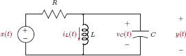

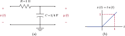
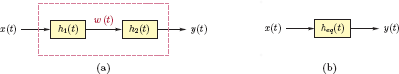
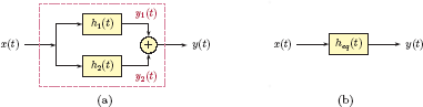
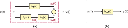
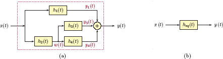

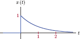
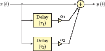
MATLAB Problems
2.32. Refer to Problem 2.2. The cascade combination of the two subsystems will be tested using the input signal
Write a MATLAB script to do the following:
- Create an anonymous anonymous function “x” to compute the input signal at all time instants specified in a vector “t”.
- Implement the cascade system as shown in Fig. P.2.2(a). Compute the signals w(t) and y(t) in the time interval − 1 ≤ t ≤ 5 s using a time increment of 0.01 s.
- Implement the cascade system in the alternative form shown in Fig. P.2.2(b). Compute the signals and in the time interval − 1 ≤ t ≤ 5 s using a time increment of 0.01 s. Compare y(t) and .
2.33. Repeat the steps of Problem 2.32 using the subsystems described in Problem 2.3.
2.34. Consider the differential equations given in Problem 2.8. Using the Euler method, find a numerical solution for each differential equation with the specified input signal and initial condition. Refer to MATLAB Exercise 2.4 for an example of doing this. For each case use a step size Ts equal to 10 percent of the time constant, and obtain the numerical solution in the time interval 0 ≤ t ≤ 2 s. Compare the numerical solution to the exact solution found in Problem 2.32.
Hint: Part (c) may be tricky due to the unit-impulse input signal. Approximate δ(t) using a pulse with unit area and a width equal to the step size.
2.35. Repeat Problem 2.34 using MATLAB function ode45(..) instead of the Euler method.
2.36. Refer to Problem 2.12 in which the unit-ramp response of the simple RC circuit of Fig. P.2.12(a) was determined. Since the circuit is assumed to be initially relaxed, it is linear and time-invariant. As a result, the unit-ramp response obtained in Problem 2.12 can be used with superposition for finding the response of the circuit to signals with higher complexity. Consider the trapezoidal input signal shown in Fig. P.2.36.
Develop a script to do the following:
- Create an anonymous function xr(..) to compute the unit ramp function at time instants in a specified vector. You may wish to review the script developed in MATLAB Exercise 2.3 as an example.
- Create an anonymous function yr(..) to compute the unit-ramp response of the RC circuit at time instants in a specified vector.
- Express the input signal x(t) in terms of scaled and time shifted unit ramp functions, and compute it in the time interval − 1 ≤ t ≤ 5 seconds with an increment of 0.01 seconds.
- Express the response y(t) of the circuit in terms of scaled and time shifted versions of the unit-ramp response, and compute it in the same time interval with the same increment.
- Graph the input and the output signals on the same coordinate system.
2.37. Refer again to the simple RC circuit shown in Fig. P.2.12(a). In MATLAB Exercise 2.3 an anonymous function was developed for computing the unit-step response of the circuit. In Problem 2.36 a similar anonymous function was developed for computing its unit-ramp response. Consider the input signal shown in Fig. P.2.37.
Develop a MATLAB script to do the following:
- Express the input signal x(t) using a combination of scaled and time shifted unit-step and unit-ramp functions.
- Use the anonymous function yu(..) from MATLAB Exercise 2.3 and the anonymous function yr(..) from Problem 2.36. Express the output signal y(t) of the circuit in terms of scaled and time shifted versions of the unit-step response and the unit-ramp response, and compute it in the time interval − 1 ≤ t ≤ 5 seconds with an increment of 0.01 seconds.
- Graph the input and the output signals on the same coordinate system.
2.38. Write a script to verify the solution to Problem 2.23. Express the triangular waveform x(t) using an anonymous function. Afterwards compute and graph the output signal y(t) in the time interval − 1 ≤ t ≤ 5s.
2.39. Write a script to verify the solution to Problem 2.24. Express the input signal x(t) = e−t u (t) using an anonymous function. Afterwards compute and graph the output signal y(t) in the time interval − 1 ≤ t ≤ 7s.
MATLAB Projects
2.40. Consider a general second-order homogeneous differential equation
with initial conditions
The coefficients a1 and a0 of the differential equation and the initial values p1 and p2 are all real-valued, and will be left as parameters.
Let s1 and s2 be the roots of the characteristic polynomial. On paper, solve the homogeneous differential equation for the three possibilities for the roots:
- The roots are real and distinct.
- The roots are a complex conjugate pair.
- The two roots are real and equal.
Find the solution y(t) as a function of the roots s1 and s2 as well as the initial values p1 and p2.
Develop a MATLAB function ss_diff2solve(..) with the syntax
y = ss_diff2solve(a1,a0,p1,p2,t)The vector “t” contains the time instants at which the solution should be computed. The returned vector “y” holds the solution at the time instants in vector “t”so that the solution can be graphed with
plot (t,y)Your function should perform the following steps:
- Test the function ss_diff2solve(..) with the homogeneous differential equations in Problems 2.9a, b, c, Problems 2.10a, b, c, and Problem 2.11a.
2.41. Refer to the discussion in Section 2.10 regarding numerical solution of a differential equation using the Euler method. A modified version of this method is the backward Euler method which uses the approximation
instead of Eqn. (2.184). With this modification Eqn. (2.185) becomes
Consider the RC circuit problem the numerical solution of which was explored in MATLAB Exercise 2.4.
- Start with the script developed in MATLAB Exercise 2.4. Modify it so that the step size is T = 0.7 s and the approximate solution is computed and graphed for 0 < t ≤ 7 s.
- Develop a new script that uses the backward Euler method to solve the same problem. To accomplish this, start with the original differential equation and approximate the derivative on the left side with the backward difference. Simplify the resulting equation and use it in the code. Compute and graph the approximate solution using a step size of T = 0.7 s as in part (a).
- Compare the results obtained in parts (a) and (b). Notice that the step size T used in both scripts is very large compared to the time constant. How does the performance of the backward Euler method compare to that of the Euler method?
2.42. Backward Euler method can be extended to apply to second-order differential equations using the approximation
for the second derivative. Using this approximation, develop a script to compute and graph the approximate solution of the homogeneous differential equation
subject to the initial conditions
Experiment with the choice of the step size T. Compare your approximate solutions to the exact solution found in Example 2.15 part (a).
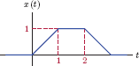
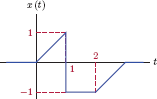
1 Another way to justify the guess utilized in Eqn. (2.73) is to write Eqn. (2.71) in the form
Integrating both sides leads to
2 cos (a + b) = cos(a) cos(b) − sin (a) sin (b).
3 Eqn. (2.146) essentially represents the superposition principle applied to an infinite sum of terms x(λ)δ (t − λ). There are studies that conclude that one may find particular signals and circumstances under which the transition from Eqn. (2.145) to Eqn. (2.146) would be problematic. For the types of signals and systems encountered in engineering practice, however, Eqn. (2.146) will generally be valid.