
State-Space Analysis of Systems
Chapter Objectives
- Understand the concepts of a state variable and state-space representation of systems.
- Learn the advantages of state-space modeling over other methods of representing continuous-time and discrete-time systems.
- Learn to derive state-space models for CTLTI and DTLTI systems from the knowledge of other system descriptions such as system function, differential equation or difference equation.
- Learn how to obtain a system function, a differential equation or a difference equation from the state-space model of a system.
- Develop techniques for solving state-space models for determining the state variables and the output signal of a system.
- Explore methods of converting a state-space model for a CTLTI system to that of a DTLTI system to allow simulation of CTLTI systems on a computer.
9.1 Introduction
In previous chapters of this text we have considered three different methods for describing a linear and time-invariant system:
- A linear constant-coefficient differential equation (or, in the case of a discrete-time system, a difference equation) involving the input and the output variables of the system in the time domain.
- A system function H (s) for a CTLTI system, or H (z) for a DTLTI system, describing the frequency-domain behavior characteristics of the system.
- An impulse response h (t) for a CTLTI system, or h [n] for a DTLTI system, that describes how the system responds to a continuous unit-impulse function δ (t) or a discrete-time unit-impulse function δ [n] as appropriate.
We know that these three descriptions are equivalent. For a continuous-time system, the system function H (s) can be obtained from the differential equation using Laplace transform techniques, specifically using the linearity and the differentiation-in-time properties of the Laplace transform. If the system under consideration is discrete, then the z-domain transfer function H (z) can be obtained from the governing difference equation in a similar manner, using the linearity and the time-shifting properties of the z-transform. Afterwards, the impulse response h (t) or h[n] can be determined from the appropriate system function using inverse transform techniques.
Alternatively, we may need to find the differential equation or the difference equation of a system specified through its impulse response. This can be achieved by simply reversing the order of steps described above. Thus, the three definition forms listed above for a linear and time-invariant system are interchangeable since we are able to go back and forth between them freely.
For signal-system interaction problems, that is, for problems involving the actions of a system on an input signal to produce an output signal, the solution of a general N-th order differential equation may be difficult or impossible to carry out analytically for anything other than fairly simple systems and input signals. Sometimes we can avoid the need to solve the differential equation, and attempt to solve the problem using frequency-domain techniques instead. This involves first translating the problem into the frequency domain, solving it in terms of transform-based descriptions of the signals and the systems involved, and finally translating the results back to the time domain. However, this approach only works for systems that have zero initial conditions, since the transfer function concept is valid for only CTLTI or DTLTI systems that are initially relaxed. Furthermore, if the system under consideration is nonlinear or time-varying or both, then the system function-based approach cannot be used at all, since system functions are only available for CTLTI or DTLTI systems.
In this chapter we will introduce yet another method for describing a system, namely state-space representation based on a set of variables called the state variables of the system.
Consider a continuous-time system that is originally described by means of a N-th order differential equation. A state-space model for such a system can be obtained by replacing the N-th order differential equation with N first-order differential equations that involve as many state variables and their derivatives. In general, the N first-order differential equations are coupled with each other, and must be solved together as a set rather than as individual equations.
Similarly, a discrete-time system that is described through a N-th order difference equation can be represented by N first-order difference equations using as many discrete-time state variables and their one-sample delayed versions.
As evident from the foregoing discussion, the state-space model of a system is a time-domain model rather than a frequency-domain one since it is derived from a differential equation or difference equation. State-space modeling of systems provides a number of advantages over other modeling techniques:
- State-space modeling provides a standard method of formulating the time-domain input-output relationship of a system independent of the order of the system.
- State-space model of a system describes the internal structure of the system, in contrast with the other description forms which simply describe the relationship between input and output signals.
- Systems with multiple inputs and/or outputs can be handled within the standard formulation we will develop in the rest of this chapter without the need to resort to special techniques that may be dependent on the topology of the system or on the number of input or output signals.
- State-space models for CTLTI and DTLTI systems are naturally suitable for use in computer simulation of these systems.
- State-space modeling also lends itself to the representation of nonlinear and/or time-varying systems, a task that is not achievable through modeling with the use of the system function or the impulse response. A N-th order differential equation or difference equation can be used for representing nonlinear and/or time-varying signals; however, computer solutions for these types of systems still necessitate the use of state-space modeling techniques.
In Section 9.2 we discuss state-space models for CTLTI systems. The discussion starts with the problem of obtaining a state-space model for a system described by means of a circuit diagram, differential equation or system function. Afterwards, methods for solving state equations are given. The problem of obtaining the system function from state equations is examined. The issue of system stability is studied from a state-space perspective. Section 9.3 repeats the topics of Section 9.2 for DTLTI systems. Conversion of the state-space model of a CTLTI system into that of an approximately equivalent DTLTI system for the purpose of simulation is the subject of Section 9.4.
9.2 State-Space Modeling of Continuous-Time Systems
Consider a single-input single-output continuous-time system described by a N-th order differential equation. Let r (t) and y (t) be the input and the output signals of the system respectively. Note that in this chapter we will change our notation a bit, and use r (t) for an input signal instead of the usual x (t). This change is needed in order to reserve the use of xi (t) for state variables as it is customary. The system under consideration can be thought of as a black box with input signal r (t), output signal y (t) and N internal variables xi (t) for i = 1,..., N as shown in Fig. 9.1.

These internal variables are the state variables or, more compactly, the states of the system under consideration. The system can be described through a set of first-order differential equations written for each state variable:
The first derivative of each state variable appears on the left side of each equation, and is set equal to some function fi [...] of all state variables and the input r (t). The equations given in Eqn. (9.1) are referred to as the state equations of the system. They describe how each state variable changes in the time domain in response to
- The input signal r (t)
- The current values of all state variables
In a sense, observing the time-domain behavior of the state variables provides us with information about the internal operation of the system. Once the N state equations are solved for the N state variables, the output signal can be found through the use of the output equation
Eqns. (9.1) and (9.2) together form a state-space model for the system.
Up to this point in our discussion we focused on a system with a single input signal r (t) and a single output signal y (t). State-space models can be extended to systems with multiple input and/or output signals in a straightforward manner. Consider a system with K input signals {ri (t); i = 1,..., K} and M output signals {yj (t); i = 1,..., M} as shown in Fig. 9.2.

The state equations given by Eqn. (9.1) can be modified as follows to represent this system through a state-space model:
Each right-side function fi [...] becomes a function of all input signals as well as the state variables. In addition to this change, the output equation given by Eqn. (9.2) needs to be replaced with a set of output equations for computing all output signals:
Thus, the functions g1 [...], g2 [...], ..., gM [...] allow the output signals to be computed from the state variables and the input signals.
In most signal-system interaction problems our main focus is on the relationship between the input and the output signals of the system. Often we are faced with one of two types of questions:
- What is the output signal of a system in response to a specified input signal?
- What system produces a specified output signal for a specified input signal?
The first question represents an analysis perspective, and the second question represents a design perspective. Even though both questions are posed with a single-input single-output system in mind, they can easily be adapted to multiple-input multiple-output systems. In answering either question, the role of state variables is an intermediate one. We will see in later parts of this chapter that a given system can have multiple state-space models that are equivalent in terms of the input-output relationships they define. They would differ from each other, however, in terms of how they model the internal structure of the system.
In some state-space models, the state variables x1 (t), ..., xN (t) chosen correspond to actual physical signals within the system. In other models they may be purely mathematical variables that do not correspond to any physical signals. If we are in a situation where we need to understand the internal workings of a system, we may want to choose state variables that correspond to actual signals within the system. If, on the other hand, our focus is solely on the input-output relationship of the system, the role of state variables is intermediate. In such a case we would choose the state variables that lead to the simplest possible structure in the state equations given by Eqn. 9.1.
9.2.1 State-space models for CTLTI systems
The formulation given in Eqns. (9.1) through (9.4) was not based on any assumptions about the system under consideration. Therefore, it will apply to systems that do not necessarily have to be linear or time-invariant. If the continuous-time system is also linear and time-invariant (CTLTI), the right-side functions fi [...], i = 1, ..., N and gi [...], i = 1, ..., M are linear functions of the state variables and the input signals. For a single-input single-output CTLTI system, the state-space representation is in the form
and the output equation is in the form
Coefficients aij, bi, cj and d used in the state equations and the output equation are all constants independent of the time variable. Eqns. (9.5) and (9.6) can be expressed in matrix notation as follows:
The coefficient matrices used in Eqns. (9.7) and (9.8) are
The vector x (t) is the state vector that consists of the N state variables:
The vector contains the derivatives of the N state variables with respect to time:
Thus, a single-input single-output CTLTI system can be uniquely described by specifying the matrix A, the vectors B and C, and the scalar d. If the initial value x (0) of the state vector is known, the state equation given by Eqn. (9.7) can be solved for x (t). Once x (t) is determined, the output signal can be found through the use of Eqn. (9.8).
Some authors use a variant of the state equation in place of Eqn. (9.7), and express x (t) as follows:
It can be shown (see Problem 9.2 at the end of this chapter) that this alternative form of the state equation can be converted into the standard form used in Eqn. (9.7) by the use of a linear transformation of the state vector, and therefore does not warrant separate analysis.
9.2.2 Obtaining state-space model from physical description
In this section we will present examples of obtaining a state-space model for a system starting with the physical relationships that exist between the signals within the system. The next two examples will illustrate this.
Example 9.1: State-space model for RLC circuit
Find a state-space model for the RLC circuit shown in Fig. 9.3 by choosing the inductor current and the capacitor voltage as the state variables.
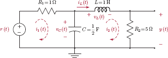
Solution: We will begin by writing KVL for the two loops:
The voltage of an inductor is proportional to the derivative of its current:
The current of a capacitor is proportional to the derivative of its voltage; therefore, we have
which can be solved for i1 (t) to yield
Substituting Eqns. (9.15) and (9.16) into Eqns. (9.13) and (9.14) and rearranging terms we obtain
The output signal is
Let the two state variables x1 (t) and x1 (t) be defined as
Using the state variables, the state equations are
and the output equation is
The state-space model in Eqns. (9.20) through (9.22) can be expressed in matrix form as
and
With the substitution of the numerical values for circuit elements we get
and
Example 9.2: State-space model for series RLC circuit
Find a state-space model for the series RLC circuit shown in Fig. 9.4.

Solution: Applying KVL to the circuit, we obtain
Using the fundamental properties of the capacitor and the inductor we have
Using them with Eqn. (9.23) we get the two state equations:
The output voltage y (t) is obtained as
We will choose the inductor current and the capacitor voltage as the state variables of the system, so we have x1 (t) = iL (t), and x2 (t) = νC (t). The state equations are
and the output equation is
The state equations and the output equation can be written in matrix form as
and
Substituting the numerical values, Eqns. (9.27) and (9.28) become
and
9.2.3 Obtaining state-space model from differential equation
Converting a N-th order differential equation to a state-space model requires finding N first-order differential equations that represent the same system, and an output equation that links the output signal to the state variables. The solution is not unique. In this section we will present just one method of accomplishing this task. Consider a CTLTI system described by a differential equation in the form
We will rewrite the differential equation so that the highest order derivative is computed from the remaining terms.
Let us choose the state variables as follows:
The resulting state equations are
The last state equation is obtained by using the state variables x1 (t) through xN (t) defined above in the differential equation given by Eqn. (9.30), and writing dxN (t)/dt in terms of the state variables x1 (t) through xN (t) and the input signal r (t). The output equation is easily found from the assignment of the first state variable:
In matrix form, the state-space model is
with
for the state equation, and
for the output equation. This form of the state-space model is called the phase-variable canonical form. It has special significance in the study of control systems. Pay attention to the structure of the coefficient matrix A, repeated below in partitioned form:

The top left partition is a (N − 1) × 1 vector of zeros; the top right partition is an identity matrix of order (N − 1); the bottom row is a vector of differential equation coefficients in reverse order and with a sign change. This is handy for obtaining the state-space model by directly inspecting the differential equation. It is important to remember, however, that the coefficient of the highest order derivative in Eqn. (9.29) must be equal to unity for this to work.
Example 9.3: State-space model from differential equation
Find a state-space model for a CTLTI system described by the differential equation
Solution: Expressing the highest order derivative as a function of the other terms leads to
State variables can be defined as
Recognizing that
the differential equation in Eqn. (9.36) can be written as
In matrix form, the state-space model is
Example 9.4: State-space model from differential equation revisited
Find a state-space model for a CTLTI system described by the differential equation
Solution: This differential equation is similar to that of Example 9.3 except for the derivative of the input signal that appears on the right side of the equal sign. While it is possible to use the alternative form of state equation suggested by Eqn. (9.12) for this system, we will choose to stay with the standard form of Eqn. (9.7). Let us first rewrite the differential equation in a rearranged form.
State variables will be defined as
We have defined the last state variable x3 (t) differently from the definition in Example 9.3 so that the left side of Eqn. (9.37) is equal to the derivative of x3 (t). Using these definitions, Eqn. (9.37) becomes
In matrix form, the state-space model is
When we compare Examples 9.3 and 9.4 we see that coefficient matrix A is the same in both of them, but the vector B is different. The inspection method for deriving the state-space model directly from the differential equation would not be as straightforward to use when we have derivatives of the input signal appearing on the right side. We will, however, generalize the relationship between the coefficients of the differential equation and the state-space model when we consider the derivation of the latter from the system function in the next section.
9.2.4 Obtaining state-space model from system function
If the CTLTI system under consideration has a system function that is simple in the sense that it has no multiple poles and all of its poles are real-valued, then a state-space model can be easily found using partial fraction expansion. This idea will be explored in the next example.
Example 9.5: State-space model from s-domain system function
It can be shown that the RLC circuit that was used in Example 9.1 and shown in Fig. 9.3 has the system function
Find an alternative, but equivalent, state-space model for the system based on this system function.
Solution: Expanding the system function into partial fractions and then solving for the transform Y (s) we get
Let us define Z1 (s) and Z2 (s) as
and
so that Y (s) = Z1 (s) + Z2 (s). Rearranging the terms in Eqns. (9.38) and (9.39) we get
and similarly
Taking the inverse Laplace transform of Eqns. (9.40) and (9.41) leads to the two first-order differential equations
Using z1 (t) and z2 (t) as the new state variables, the state-space model can be written as
and
Example 9.5 was made simple by the fact that the partial fraction expansion of the system function contains only first-order terms with real coefficients. An interesting consequence of the simple technique utilized is that the state equations obtained in Eqns. (9.42) and (9.43) are uncoupled, that is, each state equation involves only one of the state variables. This corresponds to a diagonal coefficient matrix A. Consequently, we have the advantage of being able to solve the state equations independently of each other.
If the system function does not have the properties that allowed the simple solution of Example 9.5, finding a state-space model for a system function involves the use of a block diagram as an intermediate step. The development of this idea will be presented using a third-order system function as an example; generalization to higher-order system functions will be readily apparent. Consider the system function
Using the techniques discussed in Section 7.6.1 of Chapter 7, the simulation diagram shown in Fig. 9.5 can be obtained for G (s).
We know from integration property of the Laplace transform (see Section 7.3.8 of Chapter 7) that multiplying a transform by 1/s is equivalent to integrating the corresponding signal in the time domain. Therefore, a time-domain equivalent of the block diagram in Fig. 9.5 can be obtained by replacing 1/s components with integrators and using time-domain versions of input and output quantities. The resulting diagram is shown in Fig. 9.6.

A state-space model can be obtained from the diagram of Fig. 9.4 as follows:
- Designate the output signal of each integrator as a state variable. These are marked in Fig. 9.6 as x1 (t), x2 (t) and x3 (t).
- The input of each integrator becomes the derivative of the corresponding state variable. These are marked in Fig. 9.6 as dx1/dt, dx2/dt and dx3/dt.
- Express the signal at the input of each integrator as a function of state variables and the input signal r (t) as dictated by the diagram.
Following state equations are obtained by inspecting the diagram in Fig. 9.6:
The output signal can be written as
We do not like to see the derivative of a state variable on the right side of the output equation. Substituting Eqn. (9.47 into Eqn. (9.48) yields the proper form of the output equation
Expressed in matrix form, the state-space model is
The results can easily be extended to a N-th order system function in the form
to produce the state-space model
It is interesting to see that the structure of the coefficient matrix A is the same as in Eqn. (9.35). Similarly, the vector B is identical to that found in Section 9.2.3.
Software resources: |
See MATLAB Exercise 9.1. |
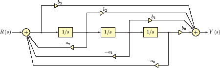
Example 9.6: State-space model from block diagram
Find a state-space model for a CTLTI system described through the system function
Solution: A block diagram for this system was constructed in Example 7.40 of Chapter 7, and was shown in Fig. 7.69. That diagram is shown again in Fig. 9.7 with notation adapted to time domain and with the designations of the four state variables marked.

The state equations are
and the output equation is
In matrix form we get
and
Example 9.7: State-space model from block diagram revisited
Find a state-space model for a CTLTI system with the system function
using the cascade form block diagram.
Solution: A cascade form block diagram for this system was constructed in Example 7.41 of Chapter 7, and was shown in Fig. 7.72. That diagram is shown again in Fig. 9.8 with notation adapted to time domain and with the designations of the four state variables marked.
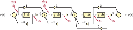
Writing the input signal of each integrator in terms of the other signals in the diagram we obtain
and the output signal is
State equations should not contain any derivatives on the right side of the equal sign. Using Eqn. (9.58) in Eqn. (9.57) yields
Similarly, using Eqn. (9.59) in Eqn. (9.56) we get
The state-space model can now be put in matrix form using Eqns. (9.55), (9.58), (9.59) and (9.60). The result is
and
9.2.5 Alternative state-space models
In Examples 9.1 and 9.2 we have defined the state variables of each system as the capacitor voltage and the inductor current. These choices were mainly motivated by the fact that the derivatives of these two quantities readily appear in KVL equations for either circuit.
Other state variables could have been defined for these systems as well, leading to alternative state-space models. Consider a CTLTI system defined through Eqns. (9.7) and (9.8). Let z (t) be a length-N column vector of variables z1 (t),..., zN (t), related to the original state vector x (t) of the CTLTI system through
where P is a constant N × N transformation matrix. The only requirement on the matrix P is that it be non-singular (invertible). Substituting Eqn. (9.61) into Eqn. (9.7) leads to
Multiplication of both sides of Eqn. (9.62) with the inverse of P from the left yields
Finally, using Eqn. (9.61) with Eqn. (9.8) we get
Eqns. (9.63) and (9.64) provide us with an alternative state-space model for the same CTLTI system, using a new state vector z (t). They can be written in the standard form of Eqns. (9.7) and (9.8) as
with newly defined coefficient matrices
and
The transformation relationship is known in control system theory as a similarity transformation. It can be used for obtaining alternative state-space models of a system. Each choice of the transformation matrix P leads to a different, but equivalent, state-space model. In each of these alternative models the input-output relationship remains the same although the state variables are different. Since any non-singular matrix P can be used in a similarity transformation, an infinite number of different state-space models can be found for a given system.
Software resources: |
See MATLAB Exercise 9.2. |
In the next several examples we will explore this concept further.
Example 9.8: Alternative state-space model for series RLC circuit
Refer to the system in Example 9.2 again. Since the system is of second order, the input-output relationship can be expressed through a second-order differential equation between y (t) and r (t). Find such a differential equation from the state-space model found in Example 9.2. Afterwards obtain an alternative state-space model for the same system directly from the second-order differential equation.
Solution: The state-space model found in Example 9.2 was
and
If we write the state equations and the output equation in open form, we obtain
Let us differentiate Eqn. (9.72) to obtain
Substituting Eqn. (9.70) into Eqn. (9.73)
Differentiating Eqn. (9.74) one more time and using the result with Eqns. (9.70) and (9.71) leads to
Finally, eliminating the state variables x1 (t) and x2 (t) between Eqns. (9.72), (9.74) and (9.75) yields the second-order differential equation
A state-space model in phase-variable canonical form can be obtained from the differential equation in Eqn. (9.76) using the technique discussed in Section 9.2.4. The result is
Software resources: |
ex_9_8.m |
Example 9.9: State variable transformation
Show that the alternative state-space model found in Example 9.8 could have been obtained from the state-space model of Example 9.2 through the transformation
Solution: The original state-space model found in Example 9.1 has the coefficient matrices
The inverse of the transformation matrix P specified above is
Applying the similarity transformation given by Eqn. (9.67) to the coefficient matrix A yields
which is identical to the matrix found in Example 9.8. Vectors and can also be found using Eqns. (9.68) and (9.69) as
and
Vectors and also agree with those found in Example 9.8.
Software resources:
ex_9_9.m
9.2.6 CTLTI systems with multiple inputs and/or outputs
A CTLTI system with multiple input and/or output signals can also be represented with a state-space model in the standard form of Eqns. (9.7 and (9.8). Consider a CTLTI system with K input signals {ri (t); i = 1,..., K} and M output signals {yj (t); i = 1,..., M}. Let r (t) be the K × 1 vector of input signals:
Similarly, y (t) is the M × 1 vector of output signals.
With these new vectors, the state equation is in the form
The matrix A is still the N × N coefficient matrix, and the vector x (t) is still the N × 1 state vector as before. Dimensions of the matrix B will need to be changed, however, to make it compatible with the K × 1 vector r (t). Therefore, B is now a N × K matrix. The output equation is in the form
Dimensions of C need to be updated as well. Since y (t) is a M × 1 vector, C is a M × N matrix. Additionally, the scalar d in the output equation in Eqn. (9.8) is replaced with a M × K matrix D.
Example 9.10: Multiple-input multiple-output system
Consider a CTLTI system with two inputs and two outputs that is described by a pair of differential equations:
Find a state-space model for this system.
Solution: We will begin by rearranging the terms of the two differential equations to obtain
Let us define the state variables as follows:
It naturally follows that
Using the definitions of the state variables in Eqns. (9.83) and (9.84) we obtain
Eqns. (9.84), (9.85) and (9.86) can be put in matrix form as
and
9.2.7 Solution of state-space model
Before deriving the general solution for the state-space model of a continuous-time system it will be useful to consider a special case in which the coefficient matrix A is upper-triangular, that is, all of its elements below the main diagonal are equal to zero. Example 9.11 will demonstrate that a step-by-step solution can be obtained in this case.
Example 9.11: Solving state equations with upper-triangular coefficient matrix
A system is described by the state-space model
and
The initial value of the state vector is
Determine the output signal in response to a unit-step input signal.
Solution: The differential equation for the state variable x3 (t) does not include either of the other two state variables; therefore, it is convenient to start with it.
Let us apply the solution technique developed in Section 2.5.1 of Chapter 2. Using Eqn. (2.57) with α = 1 and t0 = 0, the solution of Eqn. (9.87) is
Using the initial value x3 (0) = 2 and realizing that u (τ) = 1 within the integration interval we obtain
Having determined x3 (t), the differential equation for x2(t) is
Repeating the procedure outlined above,x2 (t) is determined as
Finally, the differential equation for x1 (t) is
which can be solved to yield
The output of the system is found using the output equation:
The solution of Example 9.11 was made simple by the fact that the coefficient matrix is upper-triangular. Starting with the last state equation and working our way up we were able to resolve the dependencies between state equations one at a time. Next, we will develop a general solution method that does not rely on an upper-triangular coefficient matrix. The solution will be obtained in two steps: First, the solution of the homogeneous state equation will be found. Next, a particular solution will be found based on the input signal r (t). The complete solution of the state equation is obtained as the sum of the homogeneous solution and the particular solution. The derivation of the solution procedure should be compared to the development in Section 2.5.2 of Chapter 2 for an ordinary differential equation.
Homogeneous Solution: Consider the homogeneous state equation obtained by setting r (t) = 0:
Each of the state variables xi (t) in the state vector x (t) can be expressed by a Taylor series in the form
Alternatively, Eqn. (9.93) can be generalized to construct a vector form of Taylor series for expressing the state vector x (t) as
Each vector derivative in Eqn. (9.94) corresponds to a vector of corresponding derivatives of all state variables:
Using the homogeneous state equation, the first derivative evaluated at t = 0 is
The second derivative of the state vector evaluated at time t = 0 is obtained by differentiating both sides of Eqn. (9.92) and using it in conjunction with Eqn. (9.96):
Continuing in this fashion, the n-th derivative of the state vector evaluated at t = 0 is
Using Eqn. (9.98), the Taylor series expansion given by Eqn. (9.94) for the state vector becomes
In Eqn. (9.99) the infinite series in square brackets is the matrix exponential function eAt, that is,
Therefore, the homogeneous solution of the state equation is
As in the case of scalar differential equations, the homogeneous solution represents the behavior of the state variables of the system due to the initial conditions alone. In the absence of an external input signal r (t) the matrix eAt transforms the state vector at time t = 0 to the state vector at time t. Consequently it is referred to as the state transition matrix. A method for computing the state transition matrix of a state-space model will be presented in Section 9.2.8.
State transition matrix:
General Solution: The general solution technique for the state equation will parallel the development of the general solution for a first-order differential equation in Section 2.5.1 of Chapter 2. Consider the non-homogeneous state equation
with the initial state of the system specified at time t = t0.
We will begin with an assumed solution in the form
where s (t) is a yet undetermined column vector of time functions s1 (t),..., sN (t). Differentiation of both sides of Eqn. (9.104) with respect to time results in
Comparing Eqns. (9.105) and (9.103) leads us to the conclusion
Solving Eqn. (9.106) for yields
Integrating both sides of Eqn. (9.107) over time starting at t = t0 we obtain
Substituting Eqn. (9.108) into Eqn. (9.104) results in
The term s (t0) is obtained from Eqn. (9.104) as
and Eqn. (9.109) becomes
The state equation
is solved as
Often the initial state of a system is specified at time instant t = 0. In that case the general solution becomes
9.2.8 Computation of the state transition matrix
In the previous section it became apparent that the state transition matrix plays an important role in solving the state equations. The definition of the state transition matrix ϕ (t) is based on the infinite series
While the series is convergent, and can be used for approximating ϕ (t) for specific values of t, we still need a method for determining the analytical form of ϕ (t). Such a method will be presented in this section.
We will begin with the homogeneous state equation given by Eqn. (9.92) and take the unilateral Laplace transform of each side of it to obtain
The vector X (s) is a column vector of Laplace transforms of state variables, that is,
Rearranging terms of Eqn. (9.115) we get
The matrix I in Eqn. (9.116) represents the identity matrix or order N. Its inclusion is necessary to keep the two terms in square brackets dimensionally compatible, since we could not subtract a matrix from a scalar. Solving Eqn. (9.116) for X (s) results in
The state vector can be found by taking inverse Laplace transform of Eqn. (9.117) as
The state transition matrix ϕ (t) is found by comparing Eqns. (9.118) and (9.101):
The matrix
is called the resolvent matrix , and is the Laplace transform of the state transition matrix.
In summary, computation of the state transition matrix involves the following steps:
- Form the matrix [s I − A].
- Find the resolvent matrix Φ (s) by inverting the matrix [s I − A].
- Find the state transition matrix ϕ (t) by computing the inverse Laplace transform of Φ (s).
Example 9.12: Finding the state transition matrix
Determine the state transition matrix ϕ (t) for a system with the coefficient matrix
The first step is to construct the matrix [s I − A]:
In the next step we find the resolvent matrix Φ (s):
The state transition matrix ϕ (t) is found by taking the inverse Laplace term of each element of the resolvent matrix using partial fraction expansion.
Example 9.13: Solving state equations for RLC circuit
A state-space model for the RLC circuit in Fig. 9.3 was found in Example 9.1 as
The initial value of the state vector is
Compute the two state variables x1 (t) and x2 (t) as well as the output signal y (t) in response to a unit-step input signal.
Solution: We will begin by constructing the matrix [s I − A]:
The resolvent matrix Φ (s) is the inverse of [s I − A]:
State transition matrix φ (t) is found by taking the inverse Laplace transform of each element of the resolvent matrix through partial fraction expansion:
The state vector x (t) can now be computed through the use of Eqn. (9.114). The first term in the solution is the homogeneous solution which is
In preparation for the computation of the second term in Eqn. (9.114), which is the particular solution, we first need to compute
The particular solution is
The state vector is obtained by adding the homogeneous and particular solutions:
and the output signal is obtained through the use of the output equation:
Software resources:
ex_9_13.m
Software resources: |
See MATLAB Exercises 9.3, 9.4 and 9.5. |
9.2.9 Obtaining system function from state-space model
The problem of obtaining a state-space model of a CTLTI system from its s-domain system function was considered in Section 9.2.4. In this section we will discuss the inverse problem. Given a state-space model for a CTLTI system, determine the system function G (s).
Initially we will focus on a single-input single-output system. Let the system be defined by a state-space model in the standard form of Eqns. (9.7) and (9.8). Taking the Laplace transform of both sides of the state equation yields
X (s) is a column vector that holds the Laplace transform of each state variable:
In taking the Laplace transform of the state equation we have assumed zero initial conditions, that is,
since the system is CTLTI. Recall that the system function concept is only valid for a linear and time-invariant system. Rearranging terms of Eqn. (9.121) yields
The N × N identity matrix I is necessary to keep the two terms in parentheses compatible. Solving Eqn. (9.124) for X (s) we obtain
Next we will take the Laplace transform of the output equation and then use Eqn. (9.124) in it to obtain
The system function is found from Eqn. (9.125) as
We recognize the term (s I − A)−1 in Eqn. (9.126) as the resolvent matrix Φ (s). Therefore
Example 9.14: Obtaining the system function
Determine the system function for a CTLTI system described by the state-space model
Solution: For the specified coefficient matrix A, the resolvent matrix was determined in Example 9.13 as
Using Eqn. (9.127) the system function is
Software resources: |
See MATLAB Exercises 9.6. |
The results obtained for a single-input single-output system can easily be adapted to multiple input multiple-output systems. Consider a CTLTI system with K input signals {ri (t); i = 1,..., K} and M output signals {yj (t);i = 1,..., M}. The matrix B is (N × K), and the matrix C is (M × N). The scalar d turns into a matrix D that is (M × K). As a result, Eqn. (9.127) turns into
G(s) is a (M × K) matrix of system functions from each input to each output.
Example 9.15: System function for multiple-input multiple-output system
A 2-input 2-output system is characterized by the state-space model
Determine the system function matrix G (s).
Solution: We will begin by constructing the matrix [s I − A].
The state transition matrix is found by inverting [s I − A].
The system function matrix is
Software resources:
ex_9_15.m
9.3 State-Space Modeling of Discrete-Time Systems
Discrete-time systems can also be modeled using state variables. Consider a discrete-time system with a single input signal r [n] and a single output signal y [n]. Such a system can be modeled by means of the relationships between its input and output signals as well as N internal variables xi[n] for i = 1,..., N as shown in Fig. 9.9.
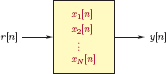
The internal variables x1[n],..., xN [n] are the state variables of the discrete-time system. Let us describe the system through a set of first-order difference equations written for each state variable:
The equations given in Eqn. (9.131) are the state equations of the system. They describe how each state variable changes in the time domain in response to
- The input signal r [n]
- The current values of all state variables
Observing the time-domain behavior of the state variables provides us with information about the internal operation of the system. Once the N state equations are solved for the N state variables, the output signal can be found through the use of the output equation
Eqns. (9.131) and (9.132) together form a state-space model for the system.
Systems with multiple inputs and/or outputs can be represented with state-space models as well. Consider a discrete-time system with K input signals {ri[n]; i = 1,..., K} and M output signals {yj[n]; i = 1,..., M} as shown in Fig. 9.10.

The state equations given by Eqn. (9.131) can be modified to apply to a multiple-input multiple-output system through a state-space model in the form
Each right-side function fi (...) includes, as arguments, all input signals as well as the state variables. In addition to this change, the output equation given by Eqn. (9.132) needs to be replaced with a set of output equations for computing all output signals:
9.3.1 State-space models for DTLTI systems
If the discrete-time system under consideration is also linear and time-invariant (DTLTI), the right-side functions fi (...), i = 1,..., N and gi (...), i = 1,..., M in Eqns. (9.133) and (9.134) are linear functions of the state variables and the input signals. For a single-input single-output DTLTI system, the state-space representation is in the form
and the output equation is
where the coefficients aij, bi, cj and d used in the state equations and the output equation are all constants independent of the time variable. Eqns. (9.135) and (9.136) can be expressed in matrix notation as follows:
The coefficient matrices used in Eqns. (9.137) and (9.138) are
The vector x [n] is the state vector that consists of the N state variables:
The vector x [n + 1] contains versions of the N state variables advanced by one sample:
Thus, a single-input single-output DTLTI system can be uniquely described by means of the matrix A, the vectors B and C, and the scalar d. If the initial value x [0] of the state vector is known, the state equation given by Eqn. (9.137) can be solved for x [n]. Once x [n] is determined, the output signal can be found through the use of Eqn. (9.138).
9.3.2 Obtaining state-space model from difference equation
Converting a N-th order difference equation to a state-space model requires finding N first-order difference equations that represent the same system, and an output equation that links the output signal to the state variables. As in the case of continuous-time state-space models, the solution is not unique. Consider a DTLTI system described by a difference equation in the form
Let us rewrite the difference equation so that y [n] is computed from the remaining terms:
We will choose the state variables as follows:
The resulting state equations are
The last state equation is obtained by using the state variables x1[n] through xN [n] defined above in the difference equation given by Eqn. (9.143), and writing y [n]= xN [n + 1] in terms of the state variables x1[n] through xN [n] and the input signal r [n]. The output equation is readily obtained from the last state equation:
In matrix form, the state-space model is
with
for the state equation, and
for the output equation. This is the familiar phase-variable canonical form we have seen in the analysis of continuous-time state-space models. The coefficient matrix A is given below in partitioned form:

The top left partition is a (N − 1) × 1 vector of zeros; the top right partition is an identity matrix of order (N − 1); the bottom row is a vector of difference equation coefficients in reverse order and with a sign change. This is handy for obtaining the state-space model by directly inspecting the difference equation. It is important to remember, however, that the coefficient of y [n] in Eqn. (9.142) must be equal to unity for this to work.
Example 9.16: State-space model from difference equation
Find a state-space model for a DTLTI system described by the difference equation
Solution: Expressing y [n] as a function of the other terms leads to
State variables can be defined as
Recognizing that
the difference equation in Eqn. (9.149) can be written as
In matrix form, the state-space model is
The inspection method for deriving the state-space model directly from the difference equation would not be as straightforward to use if delayed versions of the input signal r [n] appear in the difference equation. We will, however, generalize the relationship between the coefficients of the difference equation and the state-space model when we consider the derivation of the latter from the system function in the next section.
9.3.3 Obtaining state-space model from system function
If the DTLTI system under consideration has a system function that is simple in the sense that it has no multiple poles and all of its poles are real-valued, then a state-space model can be easily found using partial fraction expansion. This idea will be explored in the next example.
Example 9.17: State-space model from z-domain system function
A DTLTI system has the system function
Find a state-space model for this system.
Solution: Expanding H (z) into partial fractions we get
Note that we did not divide H (z) by z before expanding it into partial fractions, since in this case we do not need the z term in the numerator of each partial fraction. The z-transform of the output signal is
Let us define X1 (z) and X 2 (z) as
and
so that Y (z) = X1 (x) + X2 (z). Rearranging the terms in Eqns. (9.150) and (9.151) we get
and similarly
Taking the inverse z-transform of Eqns. (9.152) and (9.153) leads to the two first-order difference equations
The output equation is
Using x1[n] and x2[n] as the state variables, the state-space model can be written as
and
A state-space model was easily obtained for the system in Example 9.17 owing to the fact that the system function H (z) has only first-order real poles. As in the continuous-time case, the state equations obtained in Eqns. (9.154) and (9.155) are uncoupled from each other, that is, each state equation involves only one of the state variables. This leads to a state matrix A that is diagonal. It is therefore possible to solve the state equations independently of each other.
If the system function does not have the properties that afforded us the simplified solution of Example 9.17, finding a state-space model for a system function involves the use of a block diagram as an intermediate step.
Consider the system function
A direct-form II block diagram for implementing this system is shown in Fig. 9.11 (see Section 8.6 of Chapter 8 for the details of obtaining a block diagram).
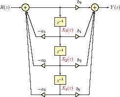
We know from time shifting property of the z-transform (see Section 8.3.2 of Chapter 8) that multiplication of a transform by z−1 is equivalent to right shifting the corresponding signal by one sample in the time domain. A time-domain equivalent of the block diagram in Fig. 9.11 is obtained by replacing z−1 components with delays and using time-domain versions of input and output quantities. The resulting diagram is shown in Fig. 9.12.

A state-space model can be obtained from the diagram of Fig. 9.134 as follows:
- Designate the output signal of each delay element as a state variable. These are marked in Fig. 9.12 as x1[n], x2[n] and x3[n].
- The input of each delay element is a one sample advanced version of the corresponding state variable. These are marked in Fig. 9.12 as x1[n + 1], x2[n + 1] and x3[n + 1].
- Express the input signal of each delay element as a function of the state variables and the input signal as dictated by the diagram.
Following state equations are obtained by inspecting the diagram:
The output signal can be written as
Since we do not want the x3[n + 1] term on the right side of the output equation, Eqn. (9.160) needs to be substituted into Eqn. (9.161) to obtain the proper output equation:
Expressed in matrix form, the state-space model is
The results can be easily extended to a N-th order system function in the form
to produce the state-space model
The structure of the coefficient matrix A is the same as in Eqn. (9.146). Similarly, the vector B is identical to that found in Section 9.3.2.
Example 9.18: State-space model from block diagram for DTLTI system
Find a state-space model for the DTLTI system described through the system function
Solution: A cascade form block diagram for this system was drawn in Example 8.43 of Chapter 8 and is shown again in Fig. 9.13 with state variable assignments marked. Writing the input signal of each delay element in terms of the other signals in the diagram we obtain

Eqn. (9.171) contains the undesired term x2[n + 1] on the right side of the equal sign. This needs to be resolved by substitution of Eqn. (9.169) into Eqn. (9.171):
The output equation is
In matrix form, the state-space model is
9.3.4 Solution of state-space model
Discrete-time state equations can be solved iteratively. Consider the state-space model given by Eqns. (9.137) and (9.138). Given the initial state vector x [0] and the input signal r[n] the iterative solution proceeds as follows:
Using n = 0, compute x [1], the state vector at n + 1 = 1 using
- Compute the output sample at n = 0 using
- Increment n by 1, and repeat steps 1 and 2.
The iterative solution method allows as many samples of the output signal to be obtained as desired. If an analytical solution is needed, however, we need to follow an alternative approach and obtain a general expression for y [n], similar to the development in Section 9.2.7 for continuous-time state-space models. It is possible to find an analytical solution by obtaining the homogeneous and particular solutions and combining them. Instead, we will use the z-transform approach. Taking the unilateral z-transform of both sides of Eqn. (9.137) we obtain
Solving Eqn. (9.174) gives
The matrix
is the z-transform version of the resolvent matrix. Using it in Eqn. (9.175) yields
for the solution in the z domain. Taking the inverse z-transform of Eqn. (9.177) and recognizing that the inverse z-transform of the product Φ (z) R(z) is the convolution of the corresponding time-domain functions leads to the solution
where ϕ [n] is the discrete-time version of the state transition matrix computed as
Example 9.19: Solution of discrete-time state-space model
Compute the unit-step response of the discrete-time system described by the state-space model
using the initial state vector
Solution: We will begin by forming the the matrix [z I − A]:
The resolvent matrix is found as
The state transition matrix is found by taking the inverse z-transform of the resolvent matrix:
The solution of the state equation is found by using the state transition matrix in Eqn. (9.178):
The output signal is
Software resources:
ex_9_19a.m
ex_9_19b.m
9.3.5 Obtaining system function from state-space model
The z-domain system function H (z) of a DTLTI system can be easily obtained from its state-space description. Consider Eqn. (9.175) derived in the process of obtaining the solution for the z-transform of the state vector:
Recall that the system function concept is valid only for a system that is both linear and time-invariant. If the system is DTLTI, then the initial value of the state vector is x[0] = 0, and Eqn. (9.175) becomes
Using X (z) in the output equation leads to
from which the system function follows as
9.4 Discretization of Continuous-Time State-Space Model
As discussed in Section 9.3.4 of this chapter, discrete-time state-space models have the added advantage that they can be solved iteratively one step at a time. On the other hand, a continuous-time state-space model cannot be solved iteratively unless it is first converted to an approximate discrete-time model. There are times when we may want to simulate an analog system on a digital computer. In this section we will discuss methods for discretizing a continuous-time state-space model. Only single-input-single-output systems will discussed although extension to systems with multiple inputs and/or outputs is straightforward. Let an analog system be described by the equations
In Eqns. (9.182) and (9.182) the subscript “a” is used to indicate analog variables. The discretization problem is stated as follows:
Given the state-space model for the analog system, find a discrete-time system with the state-space model
so that, for a sampling interval Ts we have
when r [n] = ra (nTs). The value of Ts must be chosen to satisfy the sampling criteria (see Chapter 6).
The solution for the continuous-time state-space model was given in Section 9.2.7 by Eqn. (9.113) which is repeated here:
Eqn. (9.113) starts with the solution at time t0 and returns the solution at time t. By selecting the limits of the integral to be t0 = nTs and t = (n + 1)Ts, Eqn. (9.113) becomes
If Ts is small enough the term ra (τ) may be assumed to be constant within the span of the integral, that is,
With this assumption Eqn. (9.188) becomes
Using the variable change λ = (n + 1)Ts − τ on the integral in Eqn. (9.189) we obtain
Finally, substitution of ra (nTs) = r[n] and xa (nTs) = x[n] yields
The output equation is simply
In summary, the continuous-time system described by Eqns. (9.182) and (9.183) can be approximated with the discrete-time system in Eqns. (9.184) and (9.185) by choosing the coefficient matrices as follows:
Discretization of state-space model:
Example 9.20: Discretization of state-space model for RLC circuit
A state-space model for the RLC circuit in Fig. 9.3 was found in Example 9.1 as
The state transition matrix corresponding to this model was found in Example 9.13 as
Using a step size of Ts = 0.1 s, find a discrete-time state-space model to approximate the continuous-time model given above.
Solution: Let us begin by evaluating the state transition matrix at t = Ts = 0.1 s.
The state matrix of the discrete-time model is
The inverse of state matrix A is
which can be used for computing the vector as
Therefore, the discretized state-space model for the RLC circuit in question is
Software resources:
ex_9_20.m
See MATLAB Exercise 9.8. |
The only potential drawback for the discretization technique derived above is that it requires inversion of the matrix A and computation of the state transition matrix. Simpler approximations are also available. An example of a simpler technique is the Euler method which was applied to a first-order scalar differential equation in MATLAB Exercise 2.4 in Chapter 2.
Let us evaluate the continuous-time state equation given by 9.182 at t = nTs:
The derivative on the left side of Eqn. (9.193) can be approximated using the first difference
Substituting Eqn. (9.194) into Eqn. (9.193) and rearranging terms gives
Through substitutions ra (nTs) = r[n] and xa (nTs) = x[n] we obtain
The output equation is
as before.
The results can be summarized as follows:
Discretization using Euler method:
Since this is a first-order approximation method, the step size (sampling interval) Ts chosen should be significantly small compared to the time constant.
Software resources: |
See MATLAB Exercise 9.8. |
9.5 Further Reading
[1] R.C. Dorf and R.H. Bishop. Modern Control Systems. Prentice Hall, 2011.
[2] B. Friedland. Control System Design: An Introduction to State-Space Methods. Dover Publications, 2012.
[3] K. Ogata. Modern Control Engineering. Instrumentation and Controls Series. Prentice Hall, 2010.
[4] L.A. Zadeh and C.A. Desoer. Linear System Theory: The State Space Approach. Dover Civil and Mechanical Engineering Series. Dover Publications, 2008.
MATLAB Exercises
MATLAB Exercise 9.1: Obtaining state-space model from system function
MATLAB function tf2ss(..) facilitates conversion of a rational system function in the s domain to a state-space model. Consider a CTLTI system with the system function
A state-space model for the system is obtained as
>> num = [1, 1, -2];
>> den = [1, 6, 5];
>> [A, B, C, d] = tf2ss(num, den)
A =
-6 -5
1 0
B =
1
0
C =
-5 -7
d =
1
and corresponds to
1 function [A,B,C,d] = ss_t2s (num ,den)
2 nden = length (den); % Size of denominator vector
3 N = nden - 1; % Order of system
4 % If 'num' has fewer elements than 'den', put zeros in front.
5 while (length (num)<nden)
6 num = [0, num];
7 end;
8 % Divide all coefficients by leading denominator coefficient
9 num = num/den (1);
10 den = den/den (1);
11 num = fliplr (num); % Reorder numerator coefficients
12 den = fliplr (den); % Reorder denominator coefficients
13 A = [zeros(N-1,1), eye(N-1);- den (1:N)];
14 B = [zeros(N -1 ,1);1];
15 C = num (1:N)-num(N+1)* den (1:N);
16 d = num(N+1);
17 end
After line 12 of the code is executed, the vectors “num” and “den” are structured as follows:
The construction of state-space model in lines 13 through 16 follows the development in Section 9.2.4 Eqns. (9.53) and (9.54). Using the function “ss_t2s” another state-space model for the same system is obtained as
>> num = [1,1,-2];
>> den = [1,6,5];
>> [A,B,C,d] = ss_t2s (num ,den)
A =
0 1
-5 -6
B =
0
1
C =
-7 -5
d =
1
and corresponds to
It can easily be shown (see Problem 9.9 at the end of this chapter) that this state-space model is related to the one found using MATLAB function tf2ss(..) by the transformation
Software resources:
matex_9_1a.m
matex_9_1b.m
ss_t2s.m
MATLAB Exercise 9.2: Diagonalizing the state matrix
The state-space description of a system is not unique. It was discussed in Section 9.2.5 that, for a given state-space model that uses the state vector x (t), alternative models can be obtained through similarity transformations. An alternative form using the new state vector z (t) is given by
Sometimes it is desirable to find a state-space model with a diagonal coefficient matrix so that the resulting first-order differential equations are uncoupled from each other. Let λ1, λ2, ..., λN be the eigenvalues of the matrix A with corresponding eigenvectors v1, v2, ..., vN. It can be shown that, if A has distinct eigenvalues, a transformation matrix P constructed as
leads to a state-space model with a diagonal matrix. MATLAB function eig(..) can be used to obtain both the eigenvalues and the eigenvectors.
Let the state-space model of a system be
The state-space model may be entered into MATLAB and an alternative model with a diagonal state matrix may be computed through the following:
>> A = [6.5 ,2 ,1.5; -10.5, -2, -1.5;5.5, 2, 2.5];
>> B = [1; , -2;0];
>> C = [-1,-1,-2];
>> [P,E] = eig (A);
>> A_bar = inv (P)* A*P
A_bar =
4.0000 -0.0000 -0.0000
0.0000 1.0000 0.0000
0.0000 0.0000 2.0000
>> B_bar = inv (P)* B
B_bar =
-0.0000
2.9580
-4.9749
>> C_bar = C*P
C_bar =
0.4082 0.3381 -0.0000
The results lead to a new state-space model as follows:
matex_9_2.m
MATLAB Exercise 9.3: Computation of the state transition matrix
In this exercise we will explore various approaches to the problem of computing the state transition matrix through the use of MATLAB. The definition of the state transition matrix was given by Eqn. (9.102) which is repeated here:
An infinite series form of the state transition matrix was also given, and is repeated below:
Consider the coefficient matrix A that was used in Example 9.12:
It is possible to compute the complex exponential function eAt at one specific time instant using the MATLAB function expm(..). The following segment of code computes ϕ (0.2), the value of the state transition matrix at time t = 0.2:
>> A = [-1 , -1 ,0; 1 ,0 , -1; 5 ,7 , -6];
>> expm (A *0.2)
ans =
0.8061 -0.1737 0.0126
0.1105 0.8913 -0.1105
0.5778 0.7103 0.2410
It is important to remember to use the function expm(..) and not the function exp(..) for this purpose. The latter function computes the exponential function of each element of the matrix which is not the same as computing eAt.
It is also possible to approximate the state transition matrix by using the first few terms of the infinite series for it. The infinite series can be written in nested form as
The following code segment computes the first five terms of the series for ϕ (0.2):
>> id = eye (3);
>> At = A *0.2;
>> id+ At *(id +At /2*(id +At /3*(id +At /4)))
ans =
0.8057 -0.1743 0.0130
0.1093 0.8891 -0.1093
0.5727 0.7003 0.2461
Even though we have used only the first five terms, the result obtained is quite close to that obtained through the use of the function expm(..). The accuracy of the approximation can be improved by including more terms.
Both code segments listed above compute the state transition matrix at one specific time instant. If elements of the state transition matrix are needed as functions of time over a specified interval, the function expm(..) can be used within a loop. The script listed below computes and graphs ϕ12 (t), the row-1 column-2 element of the state transition matrix, in the time interval 0 ≤ t ≤ 4 sec.
1 % Script : matex_9_3a.m
2 %
3 t = [0:0.01:4]; % Set a time vector “t”
4 % Create an empty vector “phi12” to fill later
5 phi12 =[];
6 % Compute the STM for each element of vector “t”
7 for i =1: length (t),
8 time = t(i); % Pick a time instant
9 stm = expm (A* time); % Compute the STM at time instant t(i)
10 phi12 = [phi12 , stm (1 ,2)]; % Append element (1, 2) to vector “phi12”
11 end;
12 % Graph element (1 ,2) of the STM
13 plot (t, phi12);
14 grid;
15 title (’Element 1,2 of the state transition matrix ’);
16 xlabel (’t (sec)’);
The graph produced is shown in Fig. 9.14.
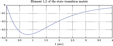
This result should be compared to the analytical expression obtained in Example 9.12 for the element ϕ12 (t):
The following code segment computes and graphs the analytical form of ϕ12 (t) for comparison:
>> phi12a = -5/3* exp (-t)+2* exp (-2* t) -1/3* exp (-4* t);
>> plot (t , phi12a);
Software resources:
matex_9_3a.m
matex_9_3b.m
MATLAB Exercise 9.4: Solving the homogeneous state equation
Consider the homogeneous state equation
Let the initial value of the state vector be
Using MATLAB, compute and graph the state transition matrix ϕ (t) in the interval 0 ≤ t ≤ 4 s. Afterwards, compute and graph the state vector x (t) in the same time interval.
Solution: The solution of the homogeneous state equation is computed as
The state transition matrix is the form
Using the state transition matrix with the initial value of the state vector we obtain
The function expm(..) was first used in MATLAB Exercise 9.3 for computing the state transition matrix at for specific value of t. In the script listed below it is used in a loop structure for computing the state transition matrix at a set of time instants. The elements of the state transition matrix are computed and graphed. The result is shown in Fig. 9.15.

1 % Script : matex_9_4a.m
2 %
3 A = [0 ,5; -2 , -2]; % State matrix
4 t = [0:0.01:4]; % Set a time vector ’t’
5 % Create empty vectors ’phi11 ’, ’phi12 ’, etc. to fill later
6 phi11 =[];
7 phi12 =[];
8 phi21 =[];
9 phi22 =[];
10 % Compute the STM for each element of vector ’t’
11 for i=1: length (t),
12 time = t(i); % Pick a time instant
13 stm = expm (A* time); % Compute the STM at time instant t(i)
14 phi11 = [phi11 , stm (1 ,1)]; % Append element (1 ,1) to vector ’phi11 ’
15 phi12 = [phi12 , stm (1 ,2)]; % Append element (1 ,2) to vector ’phi12 ’
16 phi21 = [phi21 , stm (2 ,1)]; % Append element (2 ,1) to vector ’phi21 ’
17 phi22 = [phi22 , stm (2 ,2)]; % Append element (2 ,2) to vector ’phi22 ’
18 end ;
19 % Graph elements of the STM
20 clf ;
21 subplot (2 ,2 ,1)
22 plot (t, phi11); grid ;
23 title (’ phi_ {11}(t) ’);
24 subplot (2 ,2 ,2)
25 plot (t, phi12); grid ;
26 title (’ phi_ {12}(t)’);
27 subplot (2 ,2 ,3)
28 plot (t, phi21); grid ;
29 title (’ phi_ {21}(t)’);
30 subplot (2 ,2 ,4)
31 plot (t, phi22); grid ;
32 title (’ phi_ {22}(t)’);
The script listed below computes and graphs the elements of the state vector. It relies on the previous script to be run first, so that vectors “t”, “phi11”, “phi12”,“phi21” and “phi22” are already in MATLAB workspace.
1 % Script : matex_9_4b.m
2 %
3 % Compute elements of the state vector
4 x1 = phi11 -2* phi12 ;
5 x2 = phi21 -2* phi22 ;
6 % Graph elements of the state vector
7 clf ;
8 subplot (2 ,1 ,1)
9 plot (t, x1); grid ;
10 title (’x_ {1}(t) ’);
11 subplot (2 ,1 ,2)
12 plot (t, x2); grid ;
13 title (’x_ {2}(t) ’);
The graph produced by the script matex_9_4b.m is shown in Fig. 9.16.

matex_9_4a.m
matex_9_4b.m
MATLAB Exercise 9.5: Symbolic computation of the state transition matrix
It is also possible to compute the state transition matrix using symbolic mathematics capabilities of MATLAB. This is especially useful for checking solutions to homework problems. Consider the system a state-space model of which was given in Example 9.13. The coefficient matrix is
The state transition matrix phi (t) can be computed as a symbolic expression using the following lines of code:
>> A = [-2,-2; 1,-5];
>> t = sym (’t’); % Define symbolic variable.
>> expm (A*t) % Compute the state transition matrix.
ans =
[2/ exp (3* t) - 1/ exp (4* t), 2/ exp (4* t) - 2/ exp (3* t)]
[1/ exp (3* t) - 1/ exp (4* t), 2/ exp (4* t) - 1/ exp (3* t)]
The symbolic answer produced should match the result found in Example 9.13.
An alternative approach would be to
- Obtain the resolvent matrix Φ (s).
- Obtain the state transition matrix as the inverse Laplace transform of the resolvent matrix.
Mathematically we have
The following lines of code implement this approach using the symbolic mathematics capabilities of MATLAB:
>> s = sym (’s’); % Define symbolic variable.
>> tmp = s* eye (2) - A;
>> rsm = inv (tmp) % Resolvent matrix.
rsm =
[(s + 5)/(s^2 + 7* s + 12) , -2/(s ^2 + 7* s + 12)]
[ 1/(s^2 + 7* s + 12) , (s + 2)/(s^2 + 7*s + 12)]
>> stm = ilaplace (rsm)% State transition matrix.
stm =
[2/ exp (3* t) - 1/ exp (4* t), 2/ exp (4* t) - 2/ exp (3* t)]
[1/ exp (3* t) - 1/ exp (4* t), 2/ exp (4* t) - 1/ exp (3* t)]
matex_9_5a.m
matex_9_5b.m
MATLAB Exercise 9.6: Obtaining system function from continuous-time state-space model
In Example 9.14 we have obtained the system function of a second-order CTLTI system from its state-space model. Verify the solution using symbolic mathematics capabilities of MATLAB.
Solution: Symbolic computation of the state transition matrix was discussed in MATLAB Exercise 9.5. Extending the technique used in that exercise, the system function can be found with the following statements:
>> A = [-2,-2;1,-5];
>> B = [1;0];
>> C = [0 ,5];
>> D = [0];
>> s = sym (’s’);
>> tmp = s* eye (2) - A
tmp =
[s + 2, 2]
[-1, s + 5]
>> rsm = inv (tmp)
rsm =
[(s + 5)/(s ^2 + 7* s + 12) , -2/(s ^2 + 7* s + 12)]
[ 1/(s ^2 + 7* s + 12) , (s + 2)/(s ^2 + 7* s + 12)]
>> G = C* rsm *B+D
G =
5/(s ^2 + 7* s + 12)
The system function obtained matches the result in Example 9.14.
Software resources:
matex_9_6.m
MATLAB Exercise 9.7: Obtaining system function from discrete-time state-space model
Determine the system function for a DTLTI sytem described by the state-space model
Solution: The system function H (z) can be found with the following statements:
>> A = [0 , -0.5;0.25 ,0.75];
>> B = [2;1];
>> C = [3 ,1];
>> D = [0];
>> z = sym (’z’);
>> tmp = z* eye (2) - A;
>> rsm = z* inv (tmp)
rsm =
[(2* z *(4* z - 3))/(8* z ^2 - 6* z + 1), -(4* z)/(8* z^2 - 6*z + 1)]
[ (2* z)/(8* z ^2 - 6* z + 1), (8* z ^2)/(8* z^2 - 6*z + 1)]
>> H = C* rsm *B+ D
H =
(8* z ^2)/(8* z ^2 -6* z +1) - (8* z)/(8* z ^2 -6* z +1) + (12* z *(4*z -3))/(8* z ^2 -6* z +1)
matex_9_7.m
MATLAB Exercise 9.8: Discretization of state-space model
A state-space model for the RLC circuit in Fig. 9.3 was found in Example 9.1 as
The unit-step response of the circuit was determined in Example 9.13 to be
subject to the initial state vector xa (0) = [3 − 2]T. Convert the state-space description to discrete-time, and obtain a numerical solution for the unit-step response using a sampling interval of Ts = 0.1 s.
Solution: The discrete-time state-space model can be computed with the following statements that are based on Eqn. (9.192):
>> A = [-2,-2;1,-5];
>> B = [1;0];
>> C = [0 ,5];
>> d = 0;
>> Ts = 0.1;
>> A_bar = expm (A* Ts)
A_bar =
0.8113 -0.1410
0.0705 0.5998
>> B_bar = inv (A)*(A_bar - eye (2))* B
B_bar =
0.0904
0.0040
>> C_bar = C
C_bar =
0 5
>> d_bar = d
d_bar =
0
Once coefficient matrix and vectors “A bar”, “B bar”, “C bar”, and “d bar” are created, the output signal can be approximated by iteratively solving the discrete-time state-space model. The script listed below computes the iterative solution for n = 0,..., 30. It also graphs the approximate solution found (red dots) superimposed with the analytical solution found in Example 9.13.
1 % Script : matex_9_8.m
2 %
3 Ts = 0.1;
4 A_bar = expm (A* Ts);
5 B_bar = inv (A)*(A_bar - eye (2))* B;
6 C_bar = C;
7 d_bar = d;
8 xn = [3; -2]; % Initial value of state vector
9 n = [0:30]; % Vector of indices
10 yn = []; % Empty vector to start
11 for nn =0:30 ,
12 xnp1 = A_bar * xn+ B_bar ; % ’xnp1 ’ represents x[n+1]
13 yn = [yn ,C*xn]; % Append to vector ’yn ’
14 xn = xnp1 ; % New becomes old for next iteration
15 end ;
16 % Graph correct vs. approximate solution.
17 t = [0:0.01:3];
18 ya = 5/12+70/3* exp (-3* t) -135/4* exp (-4* t); % From Example 9-13
19 plot (t,ya , ’b - ’,n*Ts ,yn ,’ro’); grid ;
20 title (’y_{a}(t) and y[n]’);
21 xlabel (’t (sec) ’);
The graph is shown in Fig. 9.17.

Software resources:
matex_9_8.m
MATLAB Exercise 9.9: Discretization using Euler method
Consider again the state-space model for the RLC circuit of Fig. 9.3 which was used in MATLAB Exercise 9.9. Convert the state-space description to discrete-time using Euler’s method., and obtain a numerical solution for the unit-step response using a sampling interval of Ts = 0.1 s. The initial state vector is xa (0) = [3 − 2]T.
Solution: The discrete-time state-space model can be computed with the following statements that are based on Eqn. (9.198):
>> A = [-2,-2;1,-5];
>> B = [1;0];
>> C = [0 ,5];
>> d = 0;
>> Ts = 0.1;
>> A_bar = eye (2)+ A*Ts
A_bar =
0.8000 -0.2000
0.1000 0.5000
>> B_bar = B*Ts ;
B_bar =
0.1000
0
>> C_bar = C
C_bar =
0 5
>> d_bar = d
d_bar =
0
The script listed below computes the iterative solution for n = 0,..., 30. It also graphs the approximate solution found (red dots) superimposed with the analytical solution found in Example 9.13.
1 % Script : matex_9_9.m
2 %
3 Ts = 0.1;
4 A_bar = eye (2)+ A*Ts ;
5 B_bar = B* Ts;
6 C_bar = C;
7 d_bar = d;
8 xn = [3; -2]; % Initial value of state vector
9 n = [0:30]; % Vector of indices
10 yn = []; % Empty vector to start
11 for nn =0:30 ,
12 xnp1 = A_bar *xn + B_bar ; % ’xnp1 ’ represents x[n+1]
13 yn = [yn ,C* xn]; % Append to vector ’yn ’
14 xn = xnp1 ; % New becomes old for next iteration
15 end ;
16 % Graph correct vs. approximate solution.
17 t = [0:0.01:3];
18 ya = 5/12+70/3* exp (-3* t) -135/4* exp (-4* t); % From Example 9-13
19 plot (t,ya , ’b- ’,n*Ts ,yn ,’ro ’); grid ;
20 title (’y_{a}(t) and y[n]’);
21 xlabel (’t (sec)’);
The graph is shown in Fig. 9.18.
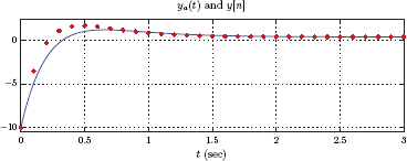
The quality of approximation is certainly not as good as the one in MATLAB Exercise 9.8, but it can be improved by reducing Ts.
Software resources:
matex_9_9.m
Problems
- 9.1. A continuous-time system is described by the following set of differential equations.
Write the state-space model of the system in matrix form.
- 9.2. Consider the alternative form of the matrix state equation given by Eqn. (9.12):
Show that this alternative form can be converted to the standard form given by Eqn. (9.7) by defining a new state vector
Express the vector F in terms of A, B and E.
The state-space model for a CTLTI system is
Convert the state-space model into the standard form by defining a new state vector z (t).
- 9.3. Find a state-space model for the circuit shown in Fig. P.9.3. Choose the capacitor voltages νC1 (t) and νC2 (t) as the state variables x1 (t) and x2 (t) respectively.
- 9.4. Find a state-space model for the RLC circuit shown in Fig. P.9.4. Choose the capacitor voltage νC (t) and the inductor current iL (t) as the state variables x1 (t) and x2 (t) respectively.
- 9.5. Using the approach taken in Examples 9.3 and 9.4 find a state-space model for each CTLTI system described by a differential equation below:
- 9.6. Find a state-space model for each CTLTI system described below by means of a system function. Use the partial fraction expansion of the system function so that the resulting state-space model has a diagonal coefficient matrix A.
- 9.7. In Example 9.4 a state-space model was obtained using an ad hoc method for the CTLTI system defined by the differential equation
Obtain a state-space model for the system using a more formal approach by
- First finding a system function G (s) for the system.
- Deriving a state space model from the system function.
- 9.8. A CTLTI system is described by the state-space model
Find a transformation matrix in the form
such that the transformation
converts the state-space model into Jordan canonical form.
- Write the state-space model in terms of the new state vector z (t).
- 9.9. Refer to MATLAB Exercise 9.1 in which two different state-space models were obtained for the same system. The first model was
and the second model was
Show that the second state-space model can be obtained from the first by means of the similarity transformation
- 9.10. Refer to Example 9.1. The state-space model obtained for the RLC circuit in Fig. 9.3 was
- Write the state equations in open form. Express dy (t)/dt and d2y (t)/dt2 in terms of the state variables x1 (t) and x2 (t) and the input signal r (t).
- Find a second-order differential equation between y (t) and r (t) by eliminating the state variables between the equations for y (t), dy (t)/dt and d2y (t)/dt2.
- Using the second-order differential equation obtained in part (b), find an alternative state-space model in phase-variable canonical form.
- 9.11. Refer to Problem 9.10. Find a similarity transformation
that would transform the original state-space model to the alternative model in phase-variable canonical form that was found.
- 9.12. Refer again to Example 9.1 in which a state-space model for the RLC circuit in Fig. 9.3 was found to be
In this problem we will explore an alternative approach for finding a differential equation between the input and the output signals of the system.
- Write the state equations in open form. Take the Laplace transform of each equation (two state equations and one output equation) by making use of linearity and time differentiation properties of the Laplace transform.
- Eliminate X1 (s) and X2 (s) to find an equation between Y (s) and R (s). Determine the system function G (s).
- Find a differential equation for the system from the system function found in part (b).
- 9.13. A CTLTI system with two inputs and two outputs is described by the following pair of differential equations:
Following the approach used in Example 9.10 find a state-space model for this system.
- 9.14. A CTLTI system with two inputs and two outputs is described by the state-space model
- Using the appropriate similarity transformation, find an equivalent state-space model for this system with a diagonal state matrix.
- Using the state-space model found, express output transforms Y1 (s) and Y2 (s) in terms of input transforms R1 (s) and R2 (s).
- Using the results found in part (b), write the input-output relationships of the system in the s-domain as
- 9.15. Refer to Example 9.11 in which the state variables and the output signal of a third-order system were determined in response to unit-step input signal and subject to specified initial conditions. Verify that the solutions found for each of the state variables and the output signal satisfy the state-space model and the initial conditions.
- 9.16. A continuous-time system is described by the state-space model
The initial value of the state vector is
Taking advantage of the upper-triangular property of the state matrix determine the output signal in response to a unit-step input signal. Follow the approach taken in Example 9.11.
- 9.17. Refer to the system in Problem 9.16.
- Using the appropriate similarity transformation, obtain an equivalent state-space model for the system in which the state matrix is diagonal.
- Use the alternative state-space model with the diagonal state matrix to determine the output signal in response to a unit-step input signal.
- 9.18. Consider the homogeneous state-space model
- Determine the state transition matrix ϕ (t).
Using the initial state vector
and the state transition matrix found in part (a), find x (2), the value of the state vector at time instant t = 2.
- Find x (5).
- 9.19. The general solution of the continuous-time state-space model can also be obtained using Laplace transform techniques. Let X (s) be the vector that holds the Laplace transform of each state variable.
- Take the unilateral Laplace transform of both sides of the state equation given by Eqn. (9.7) taking x (0), the initial value of the state vector, into account.
- Solve for X (s) in terms of the Laplace transform R (s) of the input signal.
- Take the Laplace transform of the output equation given by Eqn. (9.8) and substitute the solution found for X (s) to obtain the relationship between Y (s) and R (s).
Write the time-domain relationship between the output signal y (t) and the input signal r (t) remembering that
and that the product of two Laplace transforms corresponds to convolution of the corresponding signals in the time domain.
- 9.20. Refer to Example 9.13. Verify that the solutions found for the state variables and the output signal satisfy the state-space model and the specified initial conditions.
- 9.21. A state-space model for the RLC circuit of Fig. 9.4 was found in Example 9.2 as
Find the system function G (s) = Y (s)/R (s).
- 9.22. Find a state-space model for each DTLTI system described below by means of a difference equation.
- y[n] − 0.9 y[n − 1] = r[n]
- y[n] − 1.7 y [n − 1] + 0.72 y [n − 2] = 3r [n]
- y [n] − y [n − 1] + 0.11 y[n − 2] + 0.07 y [n − 3] = r [n]
- 9.23. System functions for several DTLTI systems are given below. Using the technique outlined in Example 9.17 that is based on partial fraction expansion, find a state-space model for each system. Ensure that the matrix A is diagonal in each case.
- 9.24. Consider the system functions given in Problem 9.23. For each system draw a direct-form II block diagram and select the state variables. Then find a state-space model based on the block diagram.
- 9.25. Consider the DTLTI systems described below by means of their difference equations. The direct method of finding a state-space model explained in Example 9.16 would be difficult to use in this case, due to the inclusion of delayed input terms r [n − 1], r [n − 2], etc. Find a state-space model for each system in two steps: First find the system function H (z), and then find a state-space model in phase-variable canonical form by inspecting the system function.
- y[n] − 0.9 y [n − 1] = r[n] + r [n − 1]
- y[n] − 1.7 y[n − 1] + 0.72 y [n − 2] = 3 r [n] + 2r [n − 2]
- y [n] − y[n − 1] + 0.11 y[n − 2] + 0.07 y[n − 3] = r [n] − r [n − 1] + r [n − 2]
- 9.26. A discrete-time system has the state-space model
The initial value of the state vector is
The input to the system is a unit-step function, that is, r[n] = u[n]. Iteratively solve for the output signal y[n] for n = 0,..., 3.
- 9.27. A discrete-time system is described by the state-space model
- Find the resolvent matrix Φ (z).
- Find the state transition matrix ϕ [n].
- Compute the unit-step response of the system using the initial state vector
- 9.28. A discrete-time system is described by the state-space model
Find the system function H (z).
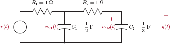

MATLAB Problems
- 9.29. A DTLTI system has the system function
Develop a MATLAB script to do the following:
- Use function tf2ss(..) to find a state-space model.
- Use function eig(..) to find a transformation matrix P that converts the state-space model found in part (a) to one with a diagonal state matrix.
- Obtain an alternative state-space model using the transformation matrix P found in part (b).
Caution: The use of the function tf2ss(..) with discrete-time system functions requires some care. Write the numerator and the denominator of the system function as polynomials of z−1, and then set up vectors for numerator and denominator coefficients for use with the function tf2ss(..).
- 9.30. Refer to the system described in Problem 9.26. Write a script to compute and graph the unit-step response of the system for n = 0,..., 99 using the iterative method.
- 9.31. Refer to the system in Problem 9.27. Write a script to determine the unit-step response of the system using symbolic mathematics functions of MATLAB. Verify the analytical solution found in Problem 9.27.
- 9.32. Refer to the system in Problem 9.28. Write a script to determine the system function H (z) using symbolic mathematics functions of MATLAB. Verify that it matches the solution found manually in Problem 9.28.
- 9.33. Repeat MATLAB Exercise 9.9 using a sampling interval of T = 0.02 s. Simulate the system for 0 ≤ t ≤ 3 s. Graph the approximated output signal against the analytical solution found in Example 9.13.
- 9.34. Consider the system a state-space model for which was found in Example 9.3.
- Find a discrete-time state-space model to approximate this system using the technique outlined in Eqns. (9.187) through (9.192). Use a sampling interval of Ts = 0.1 s.
- Using the discretized state-space model found, compute an approximation to the unit-step response of the system. Assume zero initial conditions.
- 9.35. Consider the system a state-space model for which was found in Example 9.4.