
Sampling and Reconstruction
Chapter Objectives
- Understand the concept of sampling for converting a continuous-time signal to a discrete-time signal.
- Learn how sampling affects the frequency-domain characteristics of the signal, and what precautions must be taken to ensure that the signal obtained through sampling is an accurate representation of the original.
- Consider the issue of reconstructing an analog signal from its sampled version. Understand various interpolation methods used and the spectral relationships involved in reconstruction.
- Discuss methods for changing the sampling rate of a discrete-time signal.
6.1 Introduction
The term sampling refers to the act of periodically measuring the amplitude of a continuous-time signal and constructing a discrete-time signal with the measurements. If certain conditions are satisfied, a continuous-time signal can be completely represented by measurements (samples) taken from it at uniform intervals. This allows us to store and manipulate continuous-time signals on a digital computer.
Consider, for example, the problem of keeping track of temperature variations in a classroom. The temperature of the room can be measured at any time instant, and can therefore be modeled as a continuous-time signal xa (t). Alternatively, we may choose to check the room temperature once every 10 minutes and construct a table similar to Table 6.1.
If we choose to index the temperature values with integers as shown in the third row of Table 6.1 then we could view the result as a discrete time signal x[n]in the form
Sampling the temperature signal.
Time |
8:30 |
8:40 |
8:50 |
9:00 |
9:10 |
9:20 |
9:30 |
9.40 |
Temp. (°C) |
22.4 |
22.5 |
22.8 |
21.6 |
21.7 |
21.7 |
21.9 |
22.2 |
Index n |
0 |
1 |
2 |
3 |
4 |
5 |
6 |
7 |
Thus the act of sampling allows us to obtain a discrete-time signal x[n] from the continuous-time signal xa (t). While any signal can be sampled with any time interval between consecutive samples, there are certain questions that need to be addressed before we can be confident that x[n] provides an accurate representation of xa (t). We may question, for example, the decision to wait for 10 minutes between temperature measurements. Do measurements taken 10 minutes apart provide enough information about the variations in temperature? Are we confident that no significant variations occur between consecutive measurements? If that is the case, then could we have waited for 15 minutes between measurements instead of 10 minutes?
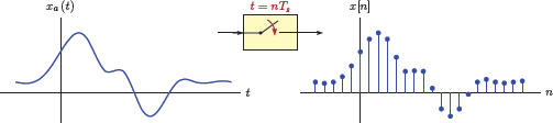
Generalizing the temperature example used above, the relationship between the continuous-time signal xa (t) and its discrete-time counterpart x[n] is
where Ts is the sampling interval, that is, the time interval between consecutive samples. It is also referred to as the sampling period. The reciprocal of the sampling interval is called the sampling rate or the sampling frequency:
The relationship between a continuous-time signal and its discrete-time version is illustrated in Fig. 6.1.
The claim that it may be possible to represent a continuous-time signal without any loss of information by a discrete set of amplitude values measured at uniformly spaced time intervals may be a bit counter-intuitive at first. How is it possible that we do not lose any information by merely measuring the signal at a discrete set of time instants and ignoring what takes place between those measurements? This question is perhaps best answered by posing another question: Does the behavior of the signal between measurement instants constitute worthwhile information, or is it just redundant behavior that could be completely predicted from the set of measurements? If it is the latter, then we will see that the measurements (samples) taken at intervals of Ts will be sufficient to reconstruct the continuous-time signal xa (t).
Sampling forms the basis of digital signals we encounter everyday in our lives. For example, an audio signal played back from a compact disc is a signal that has been captured and recorded at discrete time instants. When we look at the amplitude values stored on the disc, we only see values taken at equally spaced time instants (at a rate of 44,100 times per second) with missing amplitude values between these instants. This is perfectly fine since all the information contained in the original audio signal in the studio can be accounted for in these samples. An image captured by a digital camera is stored in the form of a dense rectangular grid of colored dots (known as pixels). When printed and viewed from an appropriate distance, we cannot tell the individual pixels apart. Similarly, a movie stored on a video cassette or a disc is stored in the form of consecutive snapshots, taken at equal time intervals. If enough snapshots are taken from the scene and are played back in sequence with the right timing, we perceive motion.
We begin by considering the sampling of continuous-time signals in Section 6.2. The idea of impulse sampling and its implications on the frequency spectrum are studied. Nyquist sampling criterion is introduced. Conversion of the impulse-sampled signal to a discrete-time signal is discussed along with the effect of the conversion on the frequency spectrum. Practical issues in sampling applications are also briefly discussed. The issue of reconstructing a continuous-time signal from its sampled version is the topic of Section 6.3. Section 6.4 covers the topic of changing the sampling rate of a signal that has already been sampled.
6.2 Sampling of a Continuous-Time Signal
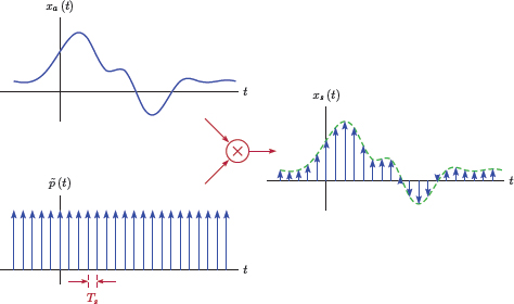
Consider a periodic impulse train p (t) with period Ts:
Multiplication of any signal x (t) with this impulse train would result in amplitude information for x (t) being retained only at integer multiples of the period Ts. Let the signal xs (t) be defined as the product of the original signal and the impulse train, i.e.,
We will refer to the signal xs (t) as the impulse-sampled version of x (t). Fig. 6.2 illustrates the relationship between the signals involved in impulse sampling.
It is important to understand that the impulse-sampled signal xs (t) is still a continuous-time signal. The subject of converting xs (t) to a discrete-time signal will be discussed in Section 6.2.2.
At this point, we need to pose a critical question: How dense must the impulse train be so that the impulse-sampled signal xs (t) is an accurate and complete representation of the original signal xa (t)? In other words, what are the restrictions on the sampling interval Ts or, equivalently, the sampling rate fs? In order to answer this question, we need to
Impulse-sampling a signal: (a) continuous-time signal x (t), (b) the pulse train p (t), (c) impulse-sampled signal xs (t).
develop some insight into how the frequency spectrum of the impulse-sampled signal xs (t) relates to the spectrum of the original signal xa (t).
Let us focus on the periodic impulse train which is shown in detail in Fig. 6.3.

As discussed in Section 4.2.3 of Chapter 4, can be represented in an exponential Fourier series expansion in the form
where ωs is both the sampling rate in rad/s and the fundamental frequency of the impulse train. It is computed as ωs = 2πfs = 2π/Ts. The EFS coefficients for are found as
Substituting the EFS coefficients found in Eqn. (6.7) into Eqn. (6.6), the impulse train becomes
Finally, using Eqn. (6.8) in Eqn. (6.5) we get
for the sampled signal xs (t). In order to determine the frequency spectrum of the impulse sampled signal xs (t) let us take the Fourier transform of both sides of Eqn. (6.9).
Linearity property of the Fourier transform was used in obtaining the result in Eqn. (6.10). Furthermore, using the frequency shifting property of the Fourier transform, the term inside the summation becomes
The frequency-domain relationship between the signal xa (t) and its impulse-sampled version xs (t) follows from Equation (6.10) and Equation (6.11).
The Fourier transform of the impulse-sampled signal is related to the Fourier transform of the original signal by
This relationship can also be written using frequencies in Hertz as
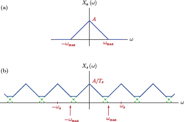
This is a very significant result. The spectrum of the impulse-sampled signal is obtained by adding frequency-shifted versions of the spectrum of the original signal, and then scaling the sum by 1/Ts. The terms of the summation in Eqn. (6.12) are shifted by all integer multiples of the sampling rate ωs. Fig. 6.4 illustrates this.
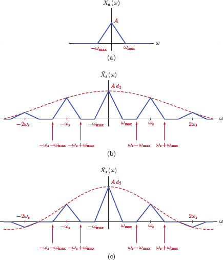
For the impulse-sampled signal to be an accurate and complete representation of the original signal, xa (t) should be recoverable from xs (t). This in turn requires that the frequency spectrum Xa (ω) be recoverable from the frequency spectrum Xs (ω). In Fig. 6.4 the example spectrum Xa (ω) used for the original signal is bandlimited to the frequency

Effects of impulse-sampling on the frequency spectrum: (a) the example spectrum Xa (ω) of the original signal xa (t), (b) the spectrum Xs (ω) of the impulse-sampled signal xs (t).
range |ω|≤ ωmax. Sampling rate ωs is chosen such that the repetitions of Xa (ω) do not overlap with each other in the construction of Xs (ω). As a result, the shape of the original spectrum Xa (ω) is preserved within the sampled spectrum Xs (ω). This ensures that xa (t) is recoverable from xs (t).
Alternatively, consider the scenario illustrated by Fig. 6.5 where the sampling rate chosen causes overlaps to occur between the repetitions of the spectrum. In this case Xa (ω) cannot be recovered from Xs (ω). Consequently, the original signal xa (t) cannot be recovered from its sampled version. Under this scenario, replacing the signal with its sampled version represents an irrecoverable loss of information.
Effects of impulse sampling on the frequency spectrum when the sampling rate chosen is too low: (a) the example spectrum Xa (ω) of the original signal xa (t), (b) the spectrum Xs (ω) of the impulse-sampled signal xs (t).
The demo program “smp_demo1.m” illustrates the process of obtaining the spectrum Xs (ω) from the original spectrum Xa (ω) based on Eqn. (6.12) and Figure 6.4 and Figure 6.5. Sampling rate fs and the bandwidth fmax of the signal to be sampled can be varied using slider controls. (In the preceding development we have used radian frequencies ωs and ωmax. They are related to related to frequencies in Hertz used by the demo program through ωs = 2πfs and ωmax = 2πfmax.)
Spectra Xa (f) and Ts Xs (f) are computed and graphed. Note that, in Fig. 6.4(b), the peak magnitude of Xs (f) is proportional to fs = 1/Ts. Same can be observed from the 1/Ts factor in Eqn. (6.12). As a result, graphing Xs (f) directly would have required a graph window tall enough to accommodate the necessary magnitude changes as the sampling rate fs = 1/Ts is varied, and still show sufficient detail. Instead, we opt to graph
to avoid the need to deal with scaling issues.
Individual terms Xa (f − kfs) in Eqn. (6.12) are also shown, although they may be under the sum Ts Xs (f), and thus invisible when the spectral sections do not overlap. When there is an overlap of spectral sections as in Fig. 6.5(b), part of each individual term becomes visible in red dashed lines. They may also be made visible by unchecking the “Show sum” box.
When spectral sections overlap, the word “Aliasing” is displayed, indicating that the spectrum is being corrupted through the sampling process.
Software resources:
smp_demo1.m
Example 6.1: Impulse sampling a right-sided exponential
Consider a right-sided exponential signal
This signal is to be impulse sampled. Determine and graph the spectrum of the impulse-sampled signal xs (t) for sampling rates fs = 200 Hz, fs = 400 Hz and fs = 600 Hz.
Solution: Using the techniques developed in Chapter 4, the frequency spectrum of the signal xa (t) is
which is graphed in Fig. 6.6(a).

Impulse-sampling xa (t) at a sampling rate of fs = /1/Ts yields the signal
The frequency spectrum of this impulse sampled signal is
which can be put into a closed form through the use of the geometric series formula (see Appendix C) as
The resulting spectrum is shown in Fig. 6.7 for fs = 200 Hz, fs = 400 Hz and fs = 600 Hz respectively.
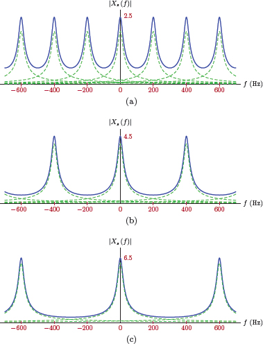
The spectrum of impulse-sampled signal for Example 6.1 (a) for fs = 200 Hz, (b) for fs = 400 Hz, (c) for fs = 600 Hz.
Note that the overlap of spectral segments (1/Ts) Xa (f − kfs) causes the shape of the spectrum Xs (f) to be different from the shape of X (f) since the right-sided exponential is not band-limited. This distortion of the spectrum is present in all three cases, but seems to be more pronounced for fs = 200 Hz than it is for the other two choices.
Software resources:
ex_6_1.m
Interactive Demo: smp_demo2
The demo program “smp_demo2.m” is based on Example 6.2. The signal xa (t)= exp (−100t)·u (t) and its impulse sampled version xs (t) are shown at the top. The bottom graph displays the magnitude of the spectrum
as well as the magnitudes of contributing terms X (f − kfs). Our logic in graphing the magnitude of Ts Xs (t) instead of Xs (t) is the same as in the previous interactive demo program “smp demo1.m”. Sampling rate fs may be adjusted using a slider control. Time and frequency domain plots are simultaneously updated to show the effect of sampling rate adjustment.
Software resources:
smp_demo2.m
Software resources: |
See MATLAB Exercise 6.1. |
6.2.1 Nyquist sampling criterion
As illustrated in Example 6.1, if the range of frequencies in the signal xa (t) is not limited, then the periodic repetition of spectral components dictated by Eqn. (6.12) creates overlapped regions. This effect is known as aliasing, and it results in the shape of the spectrum Xs (f) being different than the original spectrum Xa (f). Once the spectrum is aliased, the original signal is no longer recoverable from its sampled version. Aliasing could also occur when sampling signals that contain a finite range of frequencies if the sampling rate is not chosen carefully.
Let xa (t) be a signal the spectrum Xa (f) of which is band-limited to fmax, meaning it exhibits no frequency content for |f | >fmax. If xa (t) is impulse sampled to obtain the signal xs (t), the frequency spectrum of the resulting signal is given by Eqn. (6.12). If we want to be able to recover the signal from its impulse-sampled version, then the spectrum Xa (f) must also be recoverable from the spectrum Xs (f). This in turn requires that no overlaps occur between periodic repetitions of spectral segments. Refer to Fig. 6.8.

Determination of an appropriate sampling rate: (a) the spectrum of a properly impulse-sampled signal, (b) the spectrum of the signal with critical impulse-sampling, (c) the spectrum of the signal after improper impulse-sampling.
In order to keep the left edge of the spectral segment centered at f = fs from interfering with the right edge of the spectral segment centered at f = 0, we need
and therefore
For the impulse-sampled signal to form an accurate representation of the original signal, the sampling rate must be at least twice the highest frequency in the spectrum of the original signal. This is known as the Nyquist sampling criterion. It was named after Harry Nyquist (1889-1976) who first introduced the idea in his work on telegraph transmission. Later it was formally proven by his colleague Claude Shannon (1916-2001) in his work that formed the foundations of information theory.
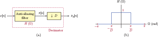
In practice, the condition in Eqn. (6.15) is usually met with inequality, and with sufficient margin between the two terms to allow for the imperfections of practical samplers and reconstruction systems. In practical implementations of samplers, the sampling rate fs is typically fixed by the constraints of the hardware used. On the other hand, the highest frequency of the actual signal to be sampled is not always known a priori. One example of this is the sampling of speech signals where the highest frequency in the signal depends on the speaker, and may vary. In order to ensure that the Nyquist sampling criterion in Eqn. (6.15) is met regardless, the signal is processed through an anti-aliasing filter before it is sampled, effectively removing all frequencies that are greater than half the sampling rate. This is illustrated in Fig. 6.9.
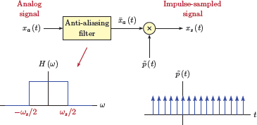
Use of an antialiasing filter to ensure compliance with the requirements of Nyquist sampling criterion.
6.2.2 DTFT of sampled signal
The relationship between the Fourier transforms of the continuous-time signal and its impulse-sampled version is given by Equation (6.12) and Equation (6.13). As discussed in Section 6.1, the purpose of sampling is to ultimately create a discrete-time signal x[n] from a continuous-time signal xa (t). The discrete-time signal can then be converted to a digital signal suitable for storage and manipulation on digital computers.
Let x[n] be defined in terms of xa (t) as
The Fourier transform of xa (t) is defined by
Similarly, the DTFT of the discrete-time signal x[n] is
We would like to understand the relationship between the two transforms in Equation (6.17) and Equation (6.18).
The impulse-sampled signal, given by Eqn. (6.5) can be written as
making use of the sampling property of the impulse function (see Eqn. (1.26) in Section 1.3.2 of Chapter 1). The Fourier transform of the impulse-sampled signal is
Interchanging the order of integration and summation, and rearranging terms, Eqn. (6.20) can be written as
Using the sifting property of the impulse function (see Eqn. (1.27) in Section 1.3.2 of Chapter 1), Eqn. (6.21) becomes
Compare Eqn. (6.22) to Eqn. (6.18). The two equations would become identical with the adjustment
This leads us to the conclusion
Using Eqn. (6.24) with Eqn. (6.12) yields the relationship between the spectrum of the original continuous-time signal and the DTFT of the discrete-time signal obtained by sampling it:
This relationship is illustrated in Fig. 6.10. It is evident from Fig. 6.10 that, in order to avoid overlaps between repetitions of the segments of the spectrum, we need
![Figure showing Relationships between the frequency spectra of the original signal and the discrete-time signal obtained from it: (a) the example spectrum Xa (ω) of the original signal xa (t), (b) the term in the summation of Eqn. (6.25) for k = 0, (c) the spectrum X (Ω) of the sampled signal x[n].](http://imgdetail.ebookreading.net/data/1/9781466598546/9781466598546__signals-and-systems__9781466598546__image__549x001.png)
Relationships between the frequency spectra of the original signal and the discrete-time signal obtained from it: (a) the example spectrum Xa (ω) of the original signal xa (t), (b) the term in the summation of Eqn. (6.25) for k = 0, (c) the spectrum X (Ω) of the sampled signal x[n].
consistent with the earlier conclusions.
Software resources: |
See MATLAB Exercise 6.2. |
6.2.3 Sampling of sinusoidal signals
In this section we consider the problem of obtaining a discrete-time sinusoidal signal by sampling a continuous-time sinusoidal signal. Let xa (t) be defined as
and let x[n] be obtained by sampling xa (t) as
Using the normalized frequency F0 = f0 Ts = f0/fs the signal x[n] becomes
The DTFT of a discrete-time sinusoidal signal was derived in Section 5.3.6 of Chapter 5, and can be applied to x[n] to yield
For the continuous-time signal xa (t) to be recoverable from x[n], the sampling rate must be chosen properly. In terms of the normalized frequency F0 we need |F0| < 0.5. Fig. 6.11 illustrates the spectrum of x[n] for proper and improper choices of the sampling rate and the corresponding normalized frequency.
The spectrum of sampled sinusoidal signal with (a) proper sampling rate, (b) improper sampling rate.
Example 6.2: Sampling a sinusoidal signal
The sinusoidal signals
are sampled using the sampling rate fs = 16 Hz and Ts = 1/fs = 0.0625 seconds to obtain the discrete-time signals
Show that the three discrete-time signals are identical, that is,
Solution: Using the specified value of Ts the signals can be written as
Incrementing the phase of a sinusoidal function by any integer multiple of 2π radians does not affect the result. Therefore, x2[n] can be written as
Since cosine is an even function, we have
Similarly, x3[n] can be written as
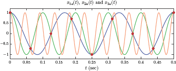
Thus, three different continuous-time signals correspond to the same discrete-time signal. Fig. 6.12 shows the three signals x1a (t), x2a (t), x3a (t) and their values at the sampling instants.
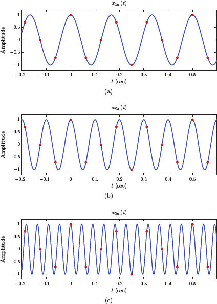
An important issue in sampling is the reconstruction of the original signal from its sampled version. Given the discrete-time signal x[n], how do we determine the continuous-time signal it represents? In this particular case we have at least three possible candidates, x1a (t), x2a (t), and x3a (t), from which x[n] could have been obtained by sampling. Other possible answers could also be found. In fact it can be shown that an infinite number of different sinusoidal signals can be passed through the points shown with red dots in Fig. 6.12. Which one is the right answer?
Let us determine the actual and the normalized frequencies for the three signals. For x1a (t) we have
Similarly for x2a (t)
and for x3a (t)
Of the three normalized frequencies only F1 satisfies the condition |F| ≤ 0.5, and the other two violate it. In terms of the Nyquist sampling theorem, the signal x1a (t) is sampled using a proper sampling rate, that is, fs > 2f1. The other two signals are sampled improperly since fs < 2f2 and fs < 2f3. Therefore, in the reconstruction process, we would pick x1a (t) based on the assumption that x[n] is a properly sampled signal. Fig. 6.13 shows the signal x2a (t) being improperly sampled with a sampling rate of fs = 16 Hz to obtain x[n]. In reconstructing the continuous-time signal from its sampled version, the signal x1a (t) is incorrectly identified as the signal that led to x[n]. This is referred to as aliasing. In this sampling scheme, x1a (t) is an alias for x2a (t).
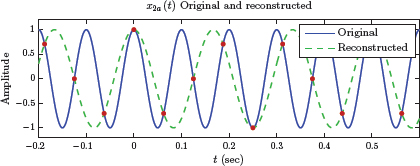
Sampling a 10 Hz sinusoidal signal with sampling rate fs = 16 Hz and attempting to reconstruct it from its sampled version.
Software resources:
ex_6_2a.m
ex_6_2b.m
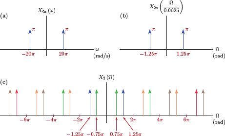
Example 6.3: Spectral relationships in sampling a sinusoidal signal
Refer to the signals in Example 6.2. Sketch the frequency spectrum for each, and then use it in obtaining the DTFT spectrum of the sampled signal.
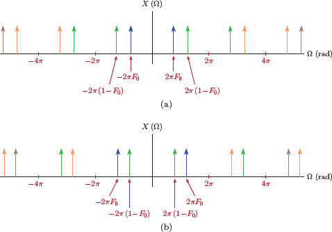
Solution: The Fourier transform of x1a (t) is
and is shown in Fig. 6.14(a). Referring to Eqn. (6.25) the term for k = 0 is
shown in Fig. 6.14(b). The spectrum of the sampled signal x1[n] is obtained as
which is shown in Fig. 6.14(c). Each impulse in X1 (Ω) has an area of 16π. The term for k = 0 is shown in blue whereas the terms for k = ∓1, k = ∓2, k = ∓3 are shown in green, orange and brown respectively. In the reconstruction process, the assumption that x1[n] is a properly sampled signal would lead us to correctly picking the two blue colored impulses at Ω = ±0.75π and ignoring the others.

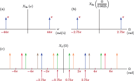
Similar analyses can be carried out for the spectra of the other two continuous-time signals x2a (t) and x3a (t) as well as the discrete-time signals that result from sampling them. Spectral relationships for these cases are shown in Figure 6.15 and Figure 6.16. Even though X1 (Ω) = X2 (Ω) = X3 (Ω) as expected, notice the differences in the contributions of the k = 0 term of Eqn. (6.25) and the others in obtaining the DTFT spectrum. In reconstructing the continuous-time signals from x2[n]and x3[n] we would also work with the assumption that the signals have been sampled properly, and incorrectly pick the green colored impulses at Ω = ±0.75π.
Interactive Demo: smp_demo3
The demo program “smp_demo3.m” is based on Example 6.2 and Example 6.3. It allows experimentation with sampling the sinusoidal signal xa (t)= cos (2πfat) to obtain a discrete-time signal x[n]. The two signals and their frequency spectra are displayed. The signal reconstructed from x[n] may also be displayed, if desired. The signal frequency fa and the sampling rate fs may be varied through the use of slider controls.
- Duplicate the results of Example 6.3 by setting the signal frequency to fa = 6 Hz and sampling rate to fs = 16 Hz. Slowly increase the signal frequency while observing the changes in the spectra of xa (t) and x[n].
- Set the signal frequency to fa = 10Hz and sampling rate to fs = 16Hz. Observe the aliasing effect. Afterwards slowly increase the sampling rate until the aliasing disappears, that is, the reconstructed signal is the same as the original.
Software resources:
smp_demo3.m
Software resources: |
See MATLAB Exercise 6.3. |
6.2.4 Practical issues in sampling
In previous sections the issue of sampling a continuous-time signal through multiplication by an impulse train was discussed. A practical consideration in the design of samplers is that we do not have ideal impulse trains, and must therefore approximate them with pulse trains. Two important questions that arise in this context are:
- What would happen to the spectrum if we used a pulse train instead of an impulse train in Eqn. (6.25)?
- How would the use of pulses affect the methods used in recovering the original signal from its sampled version?
When pulses are used instead of impulses, there are two variations of the sampling operation that can be used, namely natural sampling and zero-order hold sampling. The former is easier to generate electronically while the latter lends itself better to digital coding through techniques known as pulse-code modulation and delta modulation. We will review each sampling technique briefly.
Natural sampling
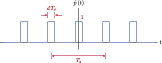
Instead of using the periodic impulse train of Eqn. (6.5), let the multiplying signal be defined as a periodic pulse train with a duty cycle of d:
where Π (t) represents a unit pulse, that is, a pulse with unit amplitude and unit width centered around the time origin t = 0. The period of the pulse train is Ts, the same as the sampling interval. The width of each pulse is dTs as shown in Fig. 6.17.
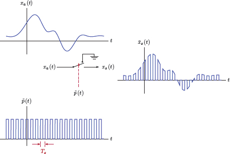
Multiplication of the signal xa (t) with yields a natural sampled version of the signal xa (t):
This is illustrated in Fig. 6.18.

An alternative way to visualize the natural sampling operation is to view the naturally sampled signal as the output of an electronic switch which is controlled by the pulse train . This implementation is shown in Fig. 6.19. The switch is closed when the pulse is present, and is opened when the pulse is absent.
In order to derive the relationship between frequency spectra of the signal xa (t) and its naturally sampled version , we will make use of the exponential Fourier series representation of .
The EFS coefficients for a pulse train with duty cycle d were found in Example 4.7 of Chapter 4 as
Therefore the EFS representation of is
Fundamental frequency is the same as the sampling rate ωs = 2π/Ts. Using Eqn. (6.33) in Eqn. (6.32) the naturally sampled signal is
The Fourier transform of the natural sampled signal is
Using Eqn. (6.34) in Eqn. (6.35) yields
Interchanging the order of integration and summation and rearranging terms we obtain
The expression in square brackets is the Fourier transform of xa (t) evaluated for ω − kωs, that is,
Substituting Eqn. (6.37) into Eqn. (6.36) yields the desired result.
Spectrum of the signal obtained through natural sampling:
The effect of natural sampling on the frequency spectrum is shown in Fig. 6.20.
Effects of natural sampling on the frequency spectrum: (a) the example spectrum Xa (ω) of the original signal xa (t), (b) the spectrum of the naturally sampled signal obtained using a pulse train with duty cycle d1, (c) the spectrum obtained using a pulse train with duty cycle d2 > d1.
It is interesting to compare the spectrum obtained in Eqn. (6.38) to the spectrum Xs (ω) given by Eqn. (6.12) for the impulse-sampled signal:
- The spectrum of the impulse-sampled signal has a scale factor of 1/Ts in front of the summation while the spectrum of the naturally sampled signal has a scale factor of d. This is not a fundamental difference. Recall that, in the multiplying signal p (t) of the impulse-sampled signal, each impulse has unit area. On the other hand, in the pulse train used for natural sampling, each pulse has a width of dTs and a unit amplitude, corresponding to an area of dTs. If we were to scale the pulse train so that each of its pulses has unit area under it, then the amplitude scale factor would have to be 1/dTs. Using in natural sampling would cause the spectrum in Eqn. (6.38) to be scaled by 1/dTs as well, matching the scaling of Xs (ω).
- As in the case of impulse sampling, frequency-shifted versions of the spectrum Xa (ω) are added together to construct the spectrum of the sampled signal. A key difference is that each term Xa (ω − kωs) is scaled by sinc (kd) as illustrated in Fig. 6.20.
Zero-order hold sampling
In natural sampling the tops of the pulses are not flat, but are rather shaped by the signal xa (t). This behavior is not always desired, especially when the sampling operation is to be followed by conversion of each pulse to digital format. An alternative is to hold the amplitude of each pulse constant, equal to the value of the signal at the left edge of the pulse. This is referred to as zero-order hold sampling or flat-top sampling, and is illustrated in Fig. 6.21.

Conceptually the signal can be modeled as the convolution of the impulse sampled signal xs (t) and a rectangular pulse with unit amplitude and a duration of dTs as shown in Fig. 6.22.

The impulse response of the zero-order hold filter in Fig. 6.22 is
Zero-order hold sampled signal can be written as
where xs (t) represents the impulse sampled signal given by Eqn. (6.5). The frequency spectrum of the zero-order hold sampled signal is found as
The system function for the zero-order hold filter is
The spectrum of the zero-order hold sampled signal is found by using Equation (6.12) and Equation (6.42) in Eqn. (6.41).
Spectrum of the signal obtained through zero-order hold sampling:
Software resources: |
See MATLAB Exercise 6.4, MATLAB Exercise 6.5 and MATLAB Exercise 6.6. |
6.3 Reconstruction of a Signal from Its Sampled Version
In previous sections of this chapter we explored the issue of sampling an analog signal to obtain a discrete-time signal. Ideally, a discrete-time signal is obtained by multiplying the analog signal with a periodic impulse train. Approximations to the ideal scenario can be obtained through the use of a pulse train instead of an impulse train.
Often the purpose of sampling an analog signal is to store, process and/or transmit it digitally, and to later convert it back to analog format. To that end, one question still remains: How can the original analog signal be reconstructed from its sampled version? Given the discrete-time signal x[n] or the impulse-sampled signal xs (t), how can we obtain a signal identical, or at least reasonably similar, to xa (t)? Obviously we need a way to “fill the gaps” between the impulses of the signal xs (t) in some meaningful way. In more technical terms, signal amplitudes between sampling instants need to be computed by some form of interpolation.
Let us first consider the possibility of obtaining a signal similar to xa (t) using rather simple methods. One such method would be to start with the impulse sampled signal xs (t) given by Eqn. (6.5) and repeated here
and to hold the amplitude of the signal equal to the value of each sample for the duration of Ts immediately following each sample. The result is a “staircase” type of approximation to the original signal. Interpolation is performed using horizontal lines, or polynomials of order zero, between sampling instants. This is referred to as zero-order hold interpolation, and is illustrated in Fig. 6.23(a), (b).
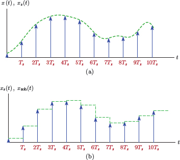
(a) Impulse sampling an analog signal x (t) to obtain xs (t), (b) reconstruction using zero-order hold interpolation.
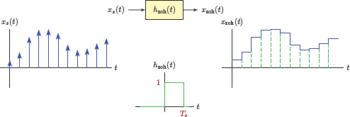
Zero-order hold interpolation can be achieved by processing the impulse sampled signal xs (t) through zero-order hold reconstruction filter, a linear system the impulse response of which is a rectangle with unit amplitude and a duration of Ts.
This is illustrated in Fig. 6.24. The linear system that performs the interpolation is called a reconstruction filter.
Notice the similarity between Eqn. (6.44) for zero-order hold interpolation and Eqn. (6.39) derived in the discussion of zero-order hold sampling. The two become the same if the duty cycle is set equal to d = 1. Therefore, the spectral relationship between the analog signal and its naturally sampled version given by Eqn. (6.43) can be used for obtaining the relationship between the analog signal and the signal reconstructed from samples using zero-order hold:
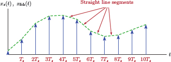
As an alternative to zero-order hold, the gaps between the sampling instants can be filled by linear interpolation, that is, by connecting the tips of the samples with straight lines as shown in Fig. 6.25. This is also known as first-order hold interpolation since the straight line segments used in the interpolation correspond to first order polynomials.
First-order hold interpolation can also be implemented using a first-order hold reconstruction filter. The impulse response of such a filter is a triangle in the form
as illustrated in Fig. 6.26.
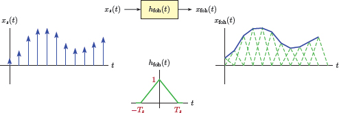
The impulse response hfoh (t) of the first-order hold interpolation filter is non-causal since it starts at t = −Ts. If a practically realizable interpolator is desired, it would be a simple matter to achieve causality by using a delayed version of hfoh (t) for the impulse response:
In this case, the reconstructed signal would naturally lag behind the sampled signal by Ts.
It is insightful to derive the frequency spectra of the reconstructed signals obtained through zero-order hold and first-order hold interpolation. For convenience we will use f rather than ω in this derivation. The system function for the zero-order hold filter is
and the spectrum of the analog signal constructed using the zero-order hold filter is
Similarly, the system function for first-order hold filter is
and the spectrum of the analog signal constructed using the first-order hold filter is
Fig. 6.27 illustrates the process of obtaining the magnitude spectrum of the output of the zero-order hold interpolation filter for the sample input spectrum used earlier in Section 6.2. Fig. 6.28 illustrates the same concept for the first-order hold interpolation filter.
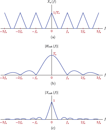
(a) Sample spectrum Xs (f) for an impulse-sampled signal, (b) magnitude spectrum |Hzoh (f) | for the zero-order hold interpolation filter, (c) magnitude spectrum |Xzoh (f) | for the signal reconstructed using zero-order hold interpolation.
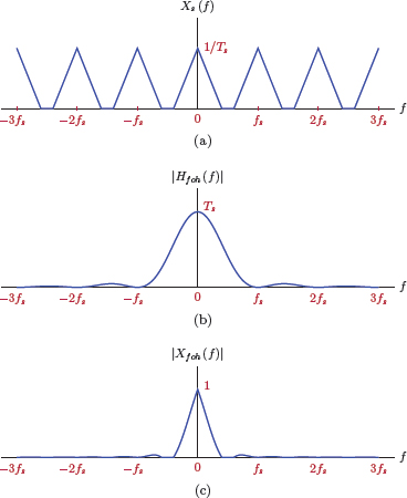
(a) Sample spectrum Xs (f) for an impulse-sampled signal, (b) magnitude spectrum |Hfoh (f) | for the first-order hold interpolation filter, (c) magnitude spectrum |Xfoh (f) | for the signal reconstructed using first-order hold interpolation.
Interestingly, both zero-order hold and first-order hold filters exhibit lowpass characteristics. A comparison of Figure 6.27(c) and Figure 6.28(c) reveals that the first-order hold interpolation filter does a better job in isolating the main section of the signal spectrum around f = 0 and suppressing spectral repetitions in Xs (f) compared to the zero-order hold interpolation filter. A comparison of the time-domain signals obtained through zero-order hold and first-order hold interpolation in Figure 6.23(b) and Figure 6.25 supports this conclusion as well. The reconstructed signal xfoh (t) is closer to the original signal xa (t) than xzoh (t) is.
The fact that both interpolation filters have lowpass characteristics warrants further exploration. The Nyquist sampling theorem states that a properly sampled signal can be recovered perfectly from its sampled version. What kind of interpolation is needed for perfect reconstruction of the analog signal from its impulse-sampled version? The answer must be found through the frequency spectrum of the sampled signal. Recall that the relationship between Xs (f), the spectrum of the impulse-sampled signal, and Xa (f), the frequency spectrum of the original signal, was found in Eqn. (6.13) to be
As long as the choice of the sampling rate satisfies the Nyquist sampling criterion, the spectrum of the impulse-sampled signal is simply a sum of frequency shifted versions of the original spectrum, shifted by every integer multiple of the sampling rate. An ideal lowpass filter that extracts the term for k = 0 from the summation in Eqn. (6.13) and suppresses all other terms for k = ±1,..., ±∞ would recover the original spectrum Xa (f), and therefore the original signal xa (t). Since the highest frequency in a properly sampled signal would be equal to or less than half the sampling rate, an ideal lowpass filter with cutoff frequency set equal to fs/2 is needed. The system function for such a reconstruction filter is
where we have also included a magnitude scaling by a factor of Ts within the system function of the lowpass filter in order to compensate for the 1/Ts term in Eqn. (6.13).

The frequency spectrum of the output of the filter defined by Eqn. (6.52) is
This is illustrated in Fig. 6.30.

Reconstruction using an ideal lowpass reconstruction filter: (a) sample spectrum Xs (f) for an impulse-sampled signal, (b) system function Hr (f) for the ideal lowpass filter with cutoff frequency fs/2, (c) spectrum Xr (f) for the signal at the output of the ideal lowpass filter.
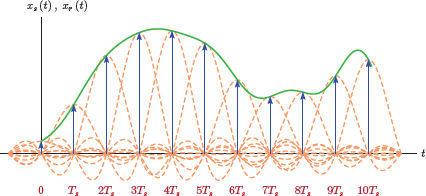
Since Xr (f) = Xa (f) we have xr (t) = xa (t). It is also interesting to determine what type of interpolation is implied in the time domain by the ideal lowpass filter of Eqn. (6.52).
The impulse response of the filter is
which, due to the sinc function, has equally-spaced zero crossings that coincide with the sampling instants. The signal at the output of the ideal lowpass filter is obtained by convolving hr (t) with the impulse-sampled signal given by Eqn. (6.5):
The nature of interpolation performed by the ideal lowpass reconstruction filter is evident from Eqn. (6.55). Let us consider the output of the filter at one of the sampling instants, say t = kTs:
We also know that
and Eqn. (6.56) becomes xr (kTs)= xa (kTs).
- The output xr (t) of the ideal lowpass reconstruction filter is equal to the sampled signal at each sampling instant.
- Between sampling instants, xr (t) is obtained by interpolation through the use of sinc functions. This is referred to as bandlimited interpolation and is illustrated in Fig. 6.31.
Up to this point we have discussed three possible methods of reconstruction by interpolating between the amplitudes of the sampled signal, namely zero-order hold, first-order hold, and bandlimited interpolation. All three methods result in reconstructed signals that have the correct amplitude values at the sampling instants, and interpolated amplitude values between them. Some interesting questions might be raised at this point:
What makes the signal obtained by bandlimited interpolation more accurate than the other two?
In a practical situation we would only have the samples xa (nTs) and would not know what the original signal xa (t) looked like between sampling instants. What if xa (t) had been identical to the zero-order hold result x zoh (t) or the first-order hold result xfoh (t) before sampling?
The answer to both questions lies in the fact that, the signal obtained by bandlimited interpolation is the only signal among the three that is limited to a bandwidth of fs/2. The bandwidth of each of the other two signals is greater than fs/2, therefore, neither of them could have been the signal that produced a properly sampled xs (t). From a practical perspective, however, both zero-order hold and first-order hold interpolation techniques are occasionally utilized in cases where exact or very accurate interpolation is not needed and simple approximate reconstruction may suffice.
Software resources: |
See MATLAB Exercises 6.7 and 6.8. |
6.4 Resampling Discrete-Time Signals
Sometimes we have the need to change the sampling rate of a discrete-time signal. Subsystems of a large scale system may operate at different sampling rates, and the ability to convert from one sampling rate to another may be necessary to get the subsystems to work together.
Consider a signal x1[n] that may have been obtained from an analog signal xa (t) by means of sampling with a sampling rate fs1= 1/T1.
Suppose an alternative version of the signal is needed, one that corresponds to sampling xa (t) with a different sampling rate fs2 =1/T2.
The question is: How can x2[n] be obtained from x1[n]?
If x1[n] is a properly sampled signal, that is, if the conditions of the Nyquist sampling theorem have been satisfied, the analog signal xa (t) may be reconstructed from it and then resampled at the new rate to obtain x 2[n]. This approach may not always be desirable or practical. Realizable reconstruction filters are far from the ideal filters called for in perfect reconstruction of the analog signal xa (t), and a loss of signal quality would occur in the conversion. We prefer to obtain x2[n] from x 1[n] using discrete-time processing methods without the need to convert x1[n] to an intermediate analog signal.
6.4.1 Reducing the sampling rate by an integer factor
Reduction of sampling rate by an integer factor D is easily accomplished by defining the signal xd[n] as
This operation is known as downsampling. The parameter D is the downsampling rate. Graphical representation of a downsampler is shown in Fig. 6.32.
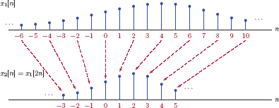
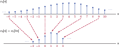
Downsampling operation was briefly discussed in Section 1.4.1 of Chapter 1 in the context of time scaling for discrete-time signals. Figs. 6.33, 6.34 and 6.35 illustrate the down-sampling of a signal using downsampling rates of D = 2 and D = 3.
![Figure showing Downsampling a signal x1[n]: (a) original signal x1[n], (b) x2[n] = x1[2n], (c) x3[n] = x1[3n].](http://imgdetail.ebookreading.net/data/1/9781466598546/9781466598546__signals-and-systems__9781466598546__image__568x002.png)
Downsampling a signal x1[n]: (a) original signal x1[n], (b) x2[n] = x1[2n], (c) x3[n] = x1[3n].
Let us consider the general downsampling relationship in Eqn. (6.31). The signal xd[n] retains one sample out of each set of D samples of the original signal. For each sample retained (D − 1) samples are discarded. The natural question that must be raised is: Are we losing information by discarding samples, or were those discarded samples just redundant or unnecessary ? In order to answer this question we need to focus on the frequency spectra of the signals involved.
Assume that the original signal was obtained by sampling an analog signal xa (t) with a samplingrate fs so that
For sampling to be appropriate, the highest frequency of the signal xa (s) must not exceed fs/2. The downsampled signal xd[n] may be obtained by sampling xa (t) with a sampling rate fs/D:
For xd[n] to represent an appropriately sampled signal the highest frequency in xa (t) must not exceed fs/2D. This is the more restricting of the two conditions on the bandwidth of xa (n) as illustrated in Fig. 6.36.
![Figure showing Spectral relationships in downsampling: (a) sample spectrum of analog signal xa (t), (b) corresponding spectrum for x[n] = xa(n/fs), (c) corresponding spectrum for xd[n] = xa (nD/fs).](http://imgdetail.ebookreading.net/data/1/9781466598546/9781466598546__signals-and-systems__9781466598546__image__570x001.png)
Spectral relationships in downsampling: (a) sample spectrum of analog signal xa (t), (b) corresponding spectrum for x[n] = xa(n/fs), (c) corresponding spectrum for xd[n] = xa (nD/fs).
The relationship between X (Ω) and Xd (Ω) could also be derived without resorting to the analog signal xa (t).
The spectrum of xd[n] is computed as
Substituting Eqn. (6.31) into Eqn. (6.31) yields
Using the variable change m =nD, Eqn. (6.31) becomes
The restriction on the index of the summation in Eqn. (6.31) makes it difficult for us to put the summation into a closed form. If a signal w [m] with the definition
is available, it can be used in Eqn. (6.31) to obtain
with no restrictions on the summation index m. Since w [m] is equal to zero for index values that are not integer multiples of D, the restriction that m be an integer multiple of D may be safely removed from the summation. It can be shown (see Problem 6.16 at the end of this chapter) that the signal w [m] can be expressed as
Using Eqn. (6.31) the spectrum of the downsampled signal xd[n] is related to the spectrum of the original signal x [n] by the following:
This result along with a careful comparison of Fig. 6.36(b) and (c) reveals that the downsampling operation could lead to aliasing through overlapping of spectral segments if care is not exercised. Spectral overlap occurs if the highest angular frequency in x [n] exceeds π/D. It is therefore customary to process the signal x [n] through a lowpass anti-aliasing filter before it is downsampled. The combination of the anti-aliasing filter and the downsampler is referred to as a decimator.
6.4.2 Increasing the sampling rate by an integer factor
In contrast with downsampling to reduce the sampling rate, the upsampling operation is used as the first step in increasing the sampling rate of a discrete-time signal. Upsampled version of a signal x [n] is defined as
where L is the upsampling rate. Graphical representation of an upsampler is shown in Fig. 6.38.
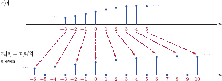
Upsampling operation was also briefly discussed in Section 1.4.1 of Chapter 1 in the context of time scaling for discrete-time signals. Fig. 6.39, illustrates the upsampling of a signal using L = 2.
Upsampling operation produces the additional samples needed for increasing the sampling rate by an integer factor; however, the new samples inserted into the signal all have zero amplitudes. Further processing is needed to change the zero-amplitude samples to more meaningful values. In order to understand what type of processing is necessary, we will again use spectral relationships. The DTFT of xu[n] is
Using the variable change n =mL, Eqn. (6.71) becomes
This result is illustrated in Fig. 6.40.
![Figure showing Spectral relationships in upsampling a signal: (a) sample spectrum of signal x[n], (b) corresponding spectrum for xu[n] = x [n/L].](http://imgdetail.ebookreading.net/data/1/9781466598546/9781466598546__signals-and-systems__9781466598546__image__573x001.png)
Spectral relationships in upsampling a signal: (a) sample spectrum of signal x[n], (b) corresponding spectrum for xu[n] = x [n/L].
A lowpass interpolation filter is needed to make the zero-amplitude samples “blend-in” with the rest of the signal. The combination of an upsampler and a lowpass interpolation filter isreferredtoasan interpolator.
Ideally, the interpolation filter should remove the extraneous spectral segments in xu (Ω) as shown in Fig. 6.42.


Spectral relationships in interpolating the upsampled signal: (a) sample spectrum of signal xu[n], (b) corresponding spectrum for u[n] at filter output.
Thus the ideal interpolation filter is a discrete-time lowpass filter with an angular cuto? frequency of Ωc = π/L and a gain of L as shown in Fig. 6.43(a). The role of the interpolation filter is similar to that of the ideal reconstruction filter discussed in Section 6.3. The impulse response of the filter is (see Problem 6.17 at the end of this chapter)
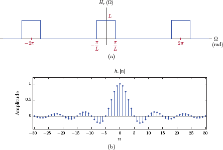
(a) Spectrum of ideal interpolation filter, (b) impulse response of ideal interpolation filter.
and is shown in Fig. 6.43(b) for the sample case of L = 5. Notice how every 5-th sample has zero amplitude so that convolution of xu[n] with this filter causes interpolation between the original samples of the signal without changing the values of the original samples.
In practical situations simpler interpolation filters may be used as well. A zero-order hold interpolation filter has the impulse response
whereas the impulse response of a first-order hold interpolation filter is
6.5 Further Reading
[1] U. Graf.Applied Laplace Transforms and Z-Transforms for Scientists and Engineers: A Computational Approach Using a Mathematica Package. Birkhäuser, 2004.
[2] D.G. Manolakis and V.K. Ingle.Applied Digital Signal Processing: Theory and Practice. Cambridge University Press, 2011.
[3] A.V. Oppenheim and R.W. Schafer.Discrete-Time Signal Processing. Prentice Hall, 2010.
[4] R.A. Schilling, R.J. Schilling, and P.D. Sandra L. Harris. Fundamentals of Digital Signal Processing Using MATLAB. Cengage Learning, 2010.
[5] L. Tan and J. Jiang. Digital Signal Processing: Fundamentals and Applications. Elsevier Science, 2013.
MATLAB Exercises
MATLAB Exercise 6.1: Spectral relations in impulse sampling
Consider the continuous-time signal
Its Fourier transform is (see Example 4.16 in Chapter 4)
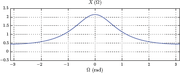
Compute and graph the spectrum of xa (t). If the signal is impulse-sampled using a sampling rate of fs = 1 Hz to obtain the signal xs (t), compute and graph the spectrum of the impulse-sampled signal. Afterwards repeat with fs =2 Hz.
Solution: The script listed below utilizes an anonymous function to define the transform xa (f). It then uses Eqn. (6.31) to compute and graph xs (f) superimposed with the contributing terms.
1 % Script : matex_6_1a.m
2 %
3 Xa = @(f) 2./(1+4* pi *pi *f.*f); % Original spectrum
4 f = [-3:0.01:3];
5 fs = 1; % Sampling rate
6 Ts = 1/fs; % Sampling interval
7 % Approximate spectrum of impulse - sampled signal
8 Xs = zeros (size(Xa(f)));
9 for k=-5:5,
10 Xs = Xs+fs*Xa(f-k*fs);
11 end;
12 % Graph the original spectrum
13 clf;
14 subplot (2, 1, 1);
15 plot (f, Xa(f)); grid;
16 axis ([-3, 3, -0.5, 2.5]);
17 title (’X_{a}(f) ’);
18 % Graph spectrum of impulse - sampled signal
19 subplot (2, 1, 2);
20 plot (f, Xs); grid;
21 axis ([-3, 3, -0.5, 2.5]);
22 hold on;
23 for k = -5:5,
24 tmp = plot (f, fs *Xa (f -k* fs), ’g:’);
25 end;
26 hold off;
27 title (’X_{s}(f) ’);
28 xlabel (’f (Hz) ’);
Lines 8 through 11 of the code approximate the spectrum xs (f) using terms for k = −5,..., 5 of the infinite summation in Eqn. (6.31). The graphs produced are shown in Fig. 6.44.

Different sampling rates may be tried easily by changing the value of the variable “fs” in line 5. The spectrum xs (f) for fs = 2 Hz is shown in Fig. 6.45.

Software resources:
matex_6_1a.m
matex_6_1b.m
MATLAB Exercise 6.2: DTFT of discrete-time signal obtained through sampling
The two-sided exponential signal
which was also used in MATLAB Exercise 6.1 is sampled using a sampling rate of fs = 1 Hz to obtain a discrete-time signal x[n]. Compute and graph X (Ω), the DTFT spectrum of x[n] for the angular frequency range −π ≤ Ωπ. Afterwards repeat with fs = 2 Hz.
Solution: The script listed below graphs the signal xa (t) and its sampled version x[n].
1 % Script : matex_6_2a.m
2 %
3 t = [−5:0.01:5];
4 xa = @(t) exp (- abs (t));
5 fs = 2;
6 Ts = 1/ fs;
7 n = [−15:15];
8 xn = xa(n*Ts);
9 clf;
10 subplot (2 ,1 ,1);
11 plot (t, xa(t)); grid ;
12 title (' Signal x_ {a}(t) '),
13 subplot (2 ,1 ,2)
14 stem (n, xn);
15 title (' Signal x[n]'),
Recall that the spectrum of the analog signal is
The DTFT spectrum X (Ω) is computed using Eqn. (6.25). The script is listed below:
1 % Script matex_6_2b.m
2 %
3 Xa = @(omg) 2./(1+ omg .* omg);
4 fs = 1;
5 Ts = 1/ fs ;
6 Omg = [−1:0.001:1]* pi;
7 XDTFT = zeros (size (Xa(Omg /Ts)));
8 for k=-5:5,
9 XDTFT = XDTFT + fs* Xa ((Omg −2* pi *k)/ Ts);
10 end ;
11 plot (Omg , XDTFT); grid ;
12 axis ([- pi ,pi , −0.5 ,2.5]);
13 title ('X ( Omega) '),
14 xlabel (' Omega (rad)'),
The graph produced is shown in Fig. 6.46.
The sampling rate fs = 2 Hz can be obtained by changing the value of the variable “fs” in line 4.
Software resources:
matex_6_2a.m
matex_6_2b.m
MATLAB Exercise 6.3: Sampling a sinusoidal signal
In Example 6.2 three sinusoidal signals
were each sampled using the sampling rate fs = 16 Hz to obtain three discrete-time signals. It was shown that the resulting signals x1[n], x2[n] and x3[n] were identical. In this exercise we will verify this result using MATLAB. The script listed below computes and displays the first few samples of each discrete-time signal:
1 % Script matex_6_3a.m
2 %
3 x1a = @(t) cos (12* pi*t);
4 x2a = @(t) cos (20* pi*t);
5 x3a = @(t) cos (44* pi*t);
6 t = [0:0.001:0.5];
7 fs = 16;
8 Ts = 1/ fs ;
9 n = [0:5];
10 x1n = x1a(n*Ts)
11 x2n = x2a(n*Ts)
12 x3n = x3a(n*Ts)
The script listed below computes and graphs the three signals and the discrete-time samples obtained by sampling them.
1 % Script : matex_6_3b.m
2 %
3 x1a = @(t) cos (12* pi*t);
4 x2a = @(t) cos (20* pi*t);
5 x3a = @(t) cos (44* pi*t);
6 t = [0:0.001:0.5];
7 fs = 16;
8 Ts = 1/ fs ;
9 n = [0:20];
10 x1n = x1a(n*Ts);
11 plot (t, x1a (t),t , x2a (t),t , x3a (t));
12 hold on ;
13 plot (n*Ts , x1n ,'ro '),
14 hold off ;
15 axis ([0 ,0.5 , −1.2 ,1.2]);
The graph produced is shown in Fig. 6.47.
matex_6_3a.m
matex_6_3b.m
MATLAB Exercise 6.4: Natural sampling
The two-sided exponential signal
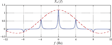
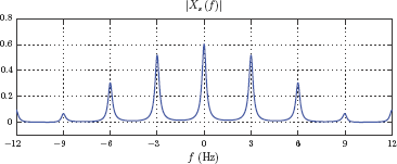
is sampled using a natural sampler with a sampling rate of fs = 4 Hz and a duty cycle of d = 0.6. Compute and graph Xs (f) in the frequency interval −12 ≤ f ≤ 12 Hz.
Solution: The spectrum given by Eqn. (6.38) may be written using f instead of ω as
The script to compute and graph s (f) is listed below. It is obtained by modifying the script “matex_6_1a.m” developed in MATLAB Exercise 6.1. The sinc envelope is also shown.
1 % Script : matex_6_4.m
2 %
3 Xa = @(f) 2./(1+4* pi *pi *f .*f);
4 f = [−12:0.01:12];
5 fs = 4; % Sampling rate.
6 Ts = 1/ fs; % sampling interval.
7 d = 0.6; % Duty cycle
8 Xs = zeros (size (Xa(f)));
9 for k = −5:5,
10 Xs = Xs + d*sinc (k*d)* Xa(f −k*fs);
11 end ;
12 plot (f,Xs , 'b−',f ,2* d* sinc (f*d/ fs), 'r-- '), grid ;
13 axis ([−12 ,12 , −0.5 ,1.5]);
The spectrum (f) is shown in Fig. 6.49.
Software resources:
matex_6_4.m
MATLAB Exercise 6.5: Zero-order hold sampling
The two-sided exponential signal
is sampled using a zero-order hold sampler with a sampling rate of fs = 3 Hz and a duty cycle of d = 0.3. Compute and graph |Xs (f)| in the frequency interval −12 ≤ f ≤ 12 Hz.
Solution: The spectrum given by Eqn. (6.43) may be written using f instead of ω as
The script to compute and graph is listed below. It is obtained by modifying the script “matex_6_1a.m.m” developed in MATLAB Exercise 6.1.
1 % Script : matex_6_5.m
2 %
3 Xa = @(f) 2./(1+4* pi* pi*f.*f);
4 f = [−12:0.01:12];
5 fs = 3; % Sampling rate
6 Ts = 1/ fs ; % Sampling interval
7 d = 0.3; % Duty cycle
8 Xs = zeros (size (Xa (f)));
9 for k = −5:5 ,
10 Xs = Xs+fs*Xa(f-k*fs);
11 end ;
12 Xs = d* Ts* sinc (f*d*Ts).* exp (-j*pi *f*d* Ts).* Xs ;
13 plot (f, abs (Xs)); grid ;
14 axis ([−12 ,12 , −0.1 ,0.8]);
15 title ('| X_s (f)| '),
16 xlabel ('f (Hz)'),
The magnitude spectrum is shown in Fig. 6.49.
Software resources:
matex_6_5.m
MATLAB Exercise 6.6: Graphing signals for natural and zero-order hold sampling
In this exercise we will develop and test two functions ss_natsamp(..) and ss_zohsamp(..) for obtaining graphical representation of signals samples using natural sampling and zero-order sampling respectively. The function ss_natsamp(..) evaluates a naturally sampled signal at a speci?ed set of time instants.
1 function xnat = ss_natsamp (xa ,Ts ,d ,t)
2 t1 = (mod(t,Ts)<=d*Ts);
3 xnat = xa (t).* t1;
4 end
The function ss_zohsamp(..) evaluates and returns a zero-order hold sampled version of the signal.
1 function xzoh = ss_zohsamp (xa ,Ts ,d ,t)
2 t1 = (mod(t,Ts)<=d*Ts);
3 xzoh = xa (t).* t1;
4 flg = 0;
5 for i = 1: length (t),
6 if not (t1 (i)) ,
7 flg = 0;
8 elseif (t1 (i) & (flg ==0)) ,
9 flg = 1;
10 value = xzoh (i);
11 end ;
12 if (flg == 1) ,
13 xzoh (i) = value ;
14 end ;
15 end ;
16 end
For both functions the input arguments are as follows:
xa: Name of an anonymous function that can be used for evaluating the analog signal xa (t) at any specified time instant.
Ts: The sampling interval in seconds.
d: The duty cycle. Should be 0 < d ≤ 1.
t: Vector of time instants at which the sampled signal should be evaluated. For a detailed graph, choose the time increment for the values in vector “t” to be significantly smaller than Ts.
The function ss_natsamp(..) can be tested with the double sided exponential signal using the following statements:
>> x = @(t) exp (- abs (t));
>> t = [−4:0.001:4];
>> xnat = ss_natsamp (x ,0.2 ,0.5 , t);
>> plot (t , xnat);
The function ss_zohsamp(..) can be tested with the following:
>> xzoh = ss_zohsamp (x ,0.2 ,0.5 , t);
>> plot (t , xzoh);
Software resources:
ss natsamp.m
ss zohsamp.m
matex_6_6a.m
matex_6_6b.m
MATLAB Exercise 6.7: Reconstruction of right-sided exponential
Recall that in Example 6.1 we considered impulse-sampling the right-sided exponential signal
The spectrum X (f) shown in Fig. 6.6 indicates that the right-sided exponential signal is not bandlimited, and therefore there is no sampling rate that would satisfy the requirements of the Nyquist sampling theorem. As a result, aliasing will be present in the spectrum regardless of the sampling rate used. In Example 6.1 three sampling rates, fs = 200 Hz, fs = 400 Hz, and fs = 600 Hz, were used. The aliasing effect is most noticeable for fs = 200 Hz, and less so for fs = 600 Hz.
In a practical application of sampling, we would have processed the signal xa (t) through an anti-aliasing ?lter prior to sampling it, as shown in Fig. 6.9. However, in this exercise we will omit the anti-aliasing ?lter, and attempt to reconstruct the signal from its sampled version using the three techniques we have discussed. The script given below produces a graph of the impulse-sampled signal and the zero-order hold approximation to the analog signal xa (t).
1 % Script : matex_6_7a.m
2 %
3 fs = 200; % Sampling rate
4 Ts = 1/ fs; % Sampling interval
5 % Set index limits "n1" and "n2" to cover the time interval
6 % from −25 ms to +75 ms
7 n1 = −fs /40;
8 n2 = −3* n1 ;
9 n = [n1 : n2];
10 t = n* Ts ; % Vector of time instants
11 xs = exp (−100* t).*(n >=0); % Samples of the signal
12 clf ;
13 stem (t,xs , '^'), grid ;
14 hold on;
15 stairs (t ,xs ,'r -'),
16 hold off ;
17 axis ([−0.030 ,0.080 , −0.2 ,1.1]);
18 title (' Reconstruction using zero - order hold '),
19 xlabel ('t (sec)'),
20 ylabel (' Amplitude '),
21 text (0.015 ,0.7 , sprintf (' Sampling rate = %.3g Hz',fs));
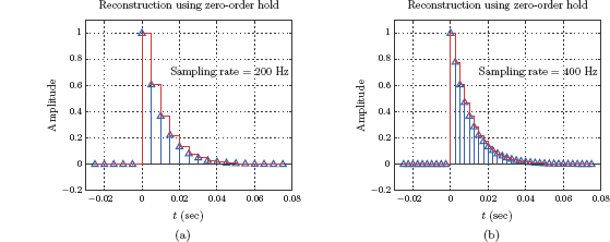
The sampling rate can be modi?ed by editing line 3 of the code. The graph generated by this function is shown in Fig. 6.51 for sampling rates 200 Hz and 400 Hz.

Impulse-sampled right-sided exponential signal and zero-order hold reconstruction for (a) fs = 200 Hz, and (b) fs = 400 Hz.
Modifying this script to produce first-order hold interpolation is almost trivial. The modified script is given below.
1 % Script : matex_6_7b.m
2 %
3 fs = 200; % Sampling rate
4 Ts = 1/ fs ; % Sampling interval
5 % Set index limits "n1" and "n2" to cover the time interval
6 % from −25 ms to +75 ms
7 n1 = −fs/40;
8 n2 = −3* n1 ;
9 n = [n1 : n2];
10 t = n*Ts; % Vector of time instants
11 xs = exp (-100* t).*(n <=0); % Samples of the signal
12 clf ;
13 stem (t,xs , '^'), grid ;
14 hold on;
15 plot (t,xs , 'r- '),
16 hold off ;
17 axis ([−0.030 ,0.080 , −0.2 ,1.1]);
18 title (' Reconstruction using first - order hold '),
19 xlabel ('t (sec)'),
20 ylabel (' Amplitude '),
21 text (0.015 ,0.7 , sprintf (' Sampling rate = %.3 g Hz ',fs));
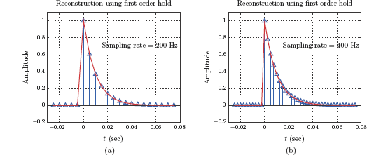
The only functional change is in line 15 where we use the function plot(..) instead of the function stairs(..). The graph generated by this modified script is shown in Fig. 6.52 for sampling rates 200 Hz and 400 Hz.
Impulse-sampled right-sided exponential signal and first-order hold reconstruction for (a) fs = 200 Hz, and (b) fs = 400 Hz.
Reconstruction through bandlimited interpolation requires a bit more work. The script for this purpose is given below. Note that we have added a new section between lines 12 and 19 to compute the shifted sinc functions called for in Eqn. (6.55).
1 % Script : matex_6_7c.m
2 %
3 fs = 200; % Sampling rate
4 Ts = 1/ fs ; % Sampling interval
5 % Set index limits "n1" and "n2" to cover the time interval
6 % from −25 ms to +75 ms
7 n1 = −fs/40;
8 n2 = −3* n1 ;
9 n = [n1 : n2];
10 t = n* Ts ; % Vector of time instants
11 xs = exp (−100* t).*(n <=0); % Samples of the signal
12 % Generate a new , more dense , set of time values for the
13 % sinc interpolating functions
14 t2 = [−0.025:0.0001:0.1];
15 xr = zeros (size (t2));
16 for n=n1:n2 ,
17 nn = n - n1 +1; % Because MATLAB indices start at 1
18 xr = xr+ xs (nn)* sinc ((t2 -n*Ts)/ Ts);
19 end ;
20 clf ;
21 stem (t,xs , '^ '), grid ;
22 hold on ;
23 plot (t2 ,xr ,'r -'),
24 hold off ;
25 axis ([−0.030 ,0.08 , −0.2 ,1.1]);
26 title (' Reconstruction using bandlimited interpolation '),
27 xlabel ('t (sec) '),
28 ylabel (' Amplitude '),
29 text (0.015 ,0.7 , sprintf (' Sampling rate = %.3 g Hz ',fs));
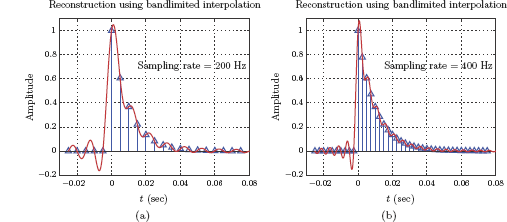
The graph generated by this script is shown in Fig. 6.53 for sampling rates 200 Hz and 400 Hz.
Impulse-sampled right-sided exponential signal and its reconstruction based on bandlimited interpolation for (a) fs = 200 Hz, and (b) fs = 400 Hz.
Software resources:
matex_6_7a.m
matex_6_7b.m
matex_6_7c.m
MATLAB Exercise 6.8: Frequency spectrum of reconstructed signal
In this exercise we will compute and graph the frequency spectra for the reconstructed signals xzoh (t), xfoh (t)and xr (t) obtained in MATLAB Exercise 6.7. Recall that the frequency spectra for the original right-sided exponential signal and its impulse-sampled version were found in Example 6.1. System functions for zero-order hold and first-order hold interpolation filters are given by Eqns. (6.48) and (6.50) respectively. Spectra for reconstructed signals are found through Eqns. (6.49) and (6.51). In the case of bandlimited interpolation, the spectrum of the reconstructed signal can be found by simply truncating the spectrum Xs (f) to retain only the part of it in the frequency range −fs/2 ≤ f = fs/2. The script listed below computes and graphs each spectrum along with the original spectrum Xa (f) for comparison. The sampling rate used in each case is fs = 200 Hz, and may be modified by editing line 3 of the code.
1 % Script : matex_6_8.m
2 %
3 fs = 200; % Sampling rate
4 Ts = 1/ fs ; % Sampling interval
5 f = [−700:0.5:700]; % Vector of frequencies
6 Xa = 1./(100+ j *2* pi *f); % Original spectrum
7 % Compute the spectrum of the impulse - sampled signal .
8 Xs = 1./(1 - exp (−100* Ts)* exp (- j *2* pi *f * Ts));
9 % Compute system functions of reconstruction filters.
10 Hzoh = Ts* sinc (f*Ts).* exp (-j*pi *Ts);
11 Hfoh = Ts* sinc (f*Ts).* sinc (f*Ts);
12 Hr = Ts *((f >= −0.5* fs)&(f <=0.5* fs));
13 % Compute spectra of reconstructed signals.
14 Xzoh = Xs .* Hzoh ; % Eqn. (6.49)
15 Xfoh = Xs.*Hfoh; % Eqn. (6.51)
16 Xr = Xs.*Hr; % Eqn. (6.53)
17 % Graph the results.
18 clf ;
19 subplot (3,1,1) ;
20 plot (f, abs(Xzoh),'-',f,abs(Xa),'--'), grid;
21 title ('Spectr. of signal reconstr. through zero-order hold'),
22 xlabel ('f (Hz)'),
23 ylabel ('Magnitude') ;
24 legend('|X_{zoh}(f)| ','|X(f)| '),
25 subplot (3,1,2);
26 plot (f, abs(Xfoh),'-',f, abs(Xa),'--'), grid;
27 title('Spectr. of signal reconstr. through first-order hold'),
28 xlabel ('f (Hz)'),
29 ylabel ('Magnitude ') ;
30 legend('|X_{foh}(f)| ','|X(f)| '),
31 subplot (3,1,3);
32 plot(f,abs(Xr),'-',f,abs(Xa),'--'), grid;
33 title('Spectr. of signal reconstr. through bandlimited interp.'),
34 xlabel ('f (Hz)'),
35 ylabel (' Magnitude ') ;
36 legend('|X_{r}(f)| ','|X(f)| '),
The graphs generated by the script are shown in Fig. 6.54. Observe the effect of aliasing on each spectrum.
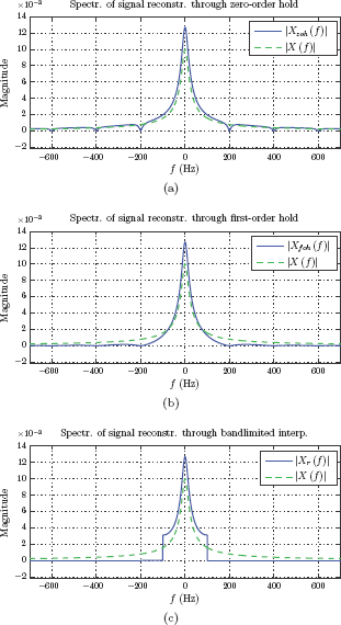
Frequency spectra of reconstructed signals obtained in MATLAB Exercise 6.8 through (a) zero-order hold, (b) first-order hold, (c) bandlimited interpolation.
Software resources:
matex_6_8.m
MATLAB Exercise 6.9: Resampling discrete-time signals
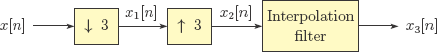
Consider the system shown in Fig. 6.55.

The input signal is
Simulate the system first without the anti-aliasing filter and then with the anti-aliasing filter. Use first-order hold interpolation after the upsampler.
Solution: The interpolation filter for first-order hold interpolation is a discrete-time triangle with a peak amplitude of 1 and the two corners at n = ∓ L = ∓4. Its impulse response is
The script listed below implements this system without the anti-aliasing filter.
1 % Script: matex_6_9a.m
2 %
3 n = [0:99];
4 x = cos(0.1*pi*n)+0.7*sin(0.2*pi*n)+cos(0.4*pi*n);
5 x1 = downsample(x ,4);
6 x2 = upsample(xd,4);
7 hr = [0,0.25,0.5,0.75,1,0.75,0.5,0.25,0]; % FOH filter
8 x3 = conv(x2,hr);
9 x3 = x3(5:104); % Compensate for 4 samples of delay
10 n = [0:99];
11 stem(n,x) ;
12 hold on;
13 plot(n,x3 ,'r') ;
14 hold off ;
15 xlabel ('n'),
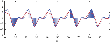
The vector “x3” obtained through convolution in line 8 has 108 samples. Line 9 of the code discards the first and the last 4 elements of “x3”. The first 4 samples discarded correspond to sample indices n = ”4,...,”1 since the impulse response hr [n] starts at index n = ”4. The last 4 samples discarded are the tail end of the convolution result. We are left with 100 samples of the signal x3[n] suitable for direct comparison with the 100-sample input signal x[n]. Input and output signals are shown in Fig. 6.56. For display purposes the output signal is shown in red with tips of samples connected by straight lines. The effect of aliasing due to the missing anti-aliasing filter is evident.

For this particular signal the implementation of an anti-aliasing filter is almost trivial. Recall from the discussion in Section 6.4.1 that the signal to be downsampled must not have any frequencies greater than Ω c = π/D = π/4. An ideal anti-aliasing filter would simply remove the third term in x [n], the term that has an angular frequency of 0.4π. In the script code we simply modify line 4 to that effect:
1 % Script: matex_6_9b.m
2 %
3 n = [0:99];
4 x = cos(0.1*pi*n)+0.7*sin(0.2*pi*n);
5 x1 = downsample(x ,4);
6 x2 = upsample(xd,4);
7 hr = [0,0.25,0.5,0.75,1,0.75,0.5,0.25,0]; % FOH filter
8 x3 = conv(x2,hr);
9 x3 = x3(5:104); % Compensate for 4 samples of delay
10 n = [0:99];
11 stem(n,x);
12 hold on;
13 plot (n,x3 , 'r ') ;
14 hold off ;
15 xlabel ('n'),
Input and output signals for this case are shown in Fig. 6.57.
matex_6_9a.m
matex_6_9b.m
Problems
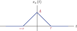
6.1. Consider the triangular waveform shown in Fig. P.6.1.
Its Fourier transform is (see Example 4.17 in Chapter 4)
Let A = 1 and τ = 1 s. The signal xa (t) is impulse-sampled using a sampling rate of fs = 5 Hz.
- Sketch the impulse-sampled signal xs (t).
- Find an expression for Xs (f).
- Sketch Xs (f) for -10 ≤ f ≤ 10 Hz.
6.2. An analog signal xa (t) has the Fourier transform shown in Fig. P.6.2.
The signal is impulse sampled using a sampling rate of fs = 100 Hz to obtain the signal xs (t). Sketch the spectrum Xs (ω).
6.3. The analog signal xa (t) with the Fourier transform shown in Fig. P.6.2 is sampled using a sampling rate of fs = 100 Hz to obtain a discrete-time signal x[n]. Sketch the spectrum X(Ω).
6.4. If the analog signal xa (t) with the Fourier transform shown in Fig. P.6.2 is sampled using a sampling rate that is 10 percent less than the minimum requirement, sketch the spectrum X (Ω).
6.5. Consider the triangular waveform xa (t) shown in Fig. P.6.1. Let A = 1 and τ = 1 s. This signal is sampled with a sampling rate of fs = 12 Hz to obtain a discrete-time signal x[n].
-
is sampled with a sampling rate of fs = 15 Hz to obtain a discrete-time signal x[n]. Determine and sketch the DTFT spectrum of x[n].
6.7. Indicate which of the following signals can be sampled without any loss of information? For signals that can be sampled properly, determine the minimum sampling rate that can be used.
- xa (t) = u(t) - u (t - 3)
- xa (t) = e-2t u (t)
- xa (t) = cos (1007πt) + 2 sin (150πf)
- xa (t) = cos (100πt) + 2 sin (150πt) sin (200πt)
- xa (t) = e-t cos (100πt)
6.8. A sinusoidal signal xa (t) = sin (2πfat) with a frequency of fa = 1 kHz is sampled using a sampling rate of fs = 2.4 kHz to obtain a discrete-time signal x[n].
- Manually sketch the signal xa (t) for the time interval 0 <t < 5 ms.
- Show the sample amplitudes of the discrete-time signal x[n] on the sketch of xa (t).
- Find three alternative frequencies for the analog signal that result in the same discrete-time signal x[n] when sampled with the sampling rate fs = 2.4kHz.
6.9. Refer to Problem 6.8.
- Sketch the frequency spectrum of the analog signal for the original sinusoid and each of the three alternative frequencies.
- For each of the signals and corresponding spectra in part (a), determine the DTFT spectrum of the discrete-time signal that results from sampling the analog signal with a sampling rate of fs = 2.4kHz.
6.10. The analog sinusoidal signal xa (t) = sin (500πt) is sampled to obtain a discrete-time signal x[n] = sin (0.4πn).
- Assuming that the signal is sampled properly, determine the sampling interval Tand the sampling rate fs.
- Find two other sampling rates that would produce the same discrete-time signal x[n].
- Using the sampling rate found in part (a), find two other analog signals that could be sampled to produce the same discrete-time signal x[n].
-
is sampled at the rate of 100 times per second to obtain a discrete-time signal x[n].
- Sketch the spectrum X(Ω) of the signal x[n].
- If we incorrectly assume that x [n] is the result of properly sampling an analog signal and try to reconstruct that analog signal, what signal would we get?
-
is sampled using natural sampling as shown in Fig. 6.18. The sampling rate used is fs = 400 Hz, and the width of each pulse is τ = 0.5ms.
- Write an analytical expression for the Fourier transform xa (ω) and sketch it.
- Find an analytical expression for the Fourier transform of the naturally-sampled signal .
- Sketch the transform .
6.13. Repeat Problem 6.12 if zero-order hold sampling is used instead of natural sampling.
6.14. The signal xa (t) = cos (150πn) is impulse-sampled with a sampling rate of fs = 200 Hz and applied to a zero-order hold reconstruction filter as shown in Fig. P.6.14.
Sketch the signal at the output of the reconstruction filter.
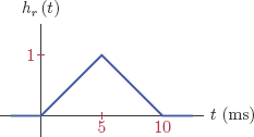
6.15. Repeat Problem 6.14 if the reconstruction filter is a delayed first-order hold filter with the impulse response shown in Fig. P.6.15.
6.16. Show that the signal w [m] defined as
and used in the derivation of the spectrum of a downsampled signal in Section 6.4 satisfies the condition
6.17. Refer to the ideal interpolation filter spectrum Hr (Ω) shown in Fig. 6.43(a). Show that the impulse response of the ideal interpolation filter is
6.18. Indicate which of the following discrete-time signals can be downsampled without any loss of information? For signals that can be downsampled properly, determine the maximum downsampling rate D that can be used.
6.19. The signal x [n] = sin (0.1πn) is applied to the system shown in Fig. P.6.19.
The interpolation filter is a zero-order hold filter with impulse response
- Find the spectrum of the zero-order hold filter.
- Determine and sketch the frequency spectra X(Ω), X1(Ω), X2 (Ω) and X3 (Ω).
6.20. Rework Problem 6.19 if the interpolation filter is changed to a first-order hold filter with impulse response


MATLAB Problems
6.21. Refer to the problem described in MATLAB Exercise 6.1.
- Set the sampling rate as fs = 3 Hz. Compute and graph the spectrum Xs (f) in the interval ”7 ≤ f ≤ 7 Hz.
- Repeat part (a) with the sampling rate set equal to fs = 4 Hz.
- Comment on the amount of aliasing for each case.
6.22. Refer to Problem 6.1. Write a script to
- Compute and graph the spectrum Xa (f).
- Compute and graph the spectrum Xs (s) for sampling rates fs = 5, 3, 2 Hz.
Use the frequency range for ”10 ≤ f ≤ 10 Hz. for all graphs.
6.23. Write a script to compute and graph the DTFT spectrum of the discrete-time signal obtained in Problem 6.5.
6.24. Write a script to compute and graph the DTFT spectrum of the discrete-time signal obtained in Problem 6.6.
6.25. Refer to Problem 6.8.
- Write a script to graph the signal xa (t) and the samples of the signal x[n] simultaneously for the time interval 0 < t < 5 ms.
- Three alternative frequencies were found that produce the same discrete-time signal. Modify the script in part (a) so that these alternative analog signals are also computed and graphed simultaneously with the original graph.
6.26. Refer to the function ss_zohsamp(..) that was developed in MATLAB Exercise 6.6.
- Explain how the function works. Pay special attention to the conditional statements between lines 6 and 14 of the code.
- The function does not work properly when the duty cycle is d = 1. Modify it so that it also works when d = 1. Assume that the sampling rate Ts is always an integer multiple of the time increment used in vector “t” and explore the use of MATLAB function kron (..) to implement the zero-order hold effect.
6.27. The two-sided exponential signal
is sampled using a zero-order hold sampler using a sampling rate of fs = 5Hzanda duty-cycle of d = 0. 9.
- Generate samples of the signal xzoh (t) for ”4 < t < 4 s using the function ss_zohsamp(..). Use a time vector with increments of 1 ms.
We will explore the possibility of obtaining a smoothly reconstructed signal from the zero-order held signal by filtering xzoh (t). A system with system function
may be simulated with statements
>> sys = tf ([a] ,[1 , a]);
>> y = lsim(sys,xzoh,t);
Compute and graph the filter output with parameter values a = 1 , 2 , 3 and comment on the results.
6.28. Write a script to simulate the system shown in Fig. P.6.19 with the input signal x[n] = sin (0.1πn) and using a zero-order hold interpolation filter. Generate 200 samples of the signal x [n]. Compute and graph the signals x1 [n], x2 [n] and x3 [n].
6.29. Write a script to repeat the simulation in Problem 6.28 using a first-order hold interpolation filter instead of the zero-order hold filter.
MATLAB Projects
6.30. In this project we will explore the concept of aliasing especially in the way it exhibits itself in an audio waveform. MATLAB has a built-in sound file named “handel” which contains a recording of Handel's Hallelujah Chorus. It was recorded with a sampling rate of fs = 8192 Hz. Use the statement
>> load handel
which loads two new variables named “Fs” and “Fs” into the workspace. The scalar variable “Fs” holds the sampling rate, and the vector “y” holds 73113 samples of the recording that corresponds to about 9 seconds of audio. Once loaded, the audio waveform may be played back with the statement
>> sound(y,Fs)
- Graph the audio signal as a function of time. Create a continuous time variable that is correctly scaled for this purpose.
- Compute and graph the frequency spectrum of the signal using the function fft(..). Create an appropriate frequency variable to display frequencies in Hertz, and use it in graphing the spectrum of the signal. Refer to the discussion in Section 5.8.5 of Chapter 5 for using the DFT to approximate the continuous Fourier transform.
- Downsample the audio signal in vector “y” using a downsampling rate of D = 2. Do not use an anti-aliasing filter for this part. Play back the resulting signal using the function sound(..). Be careful to adjust the sampling rate to reflect the act of downsampling or it will play too fast.
Repeat part (c) this time using an anti-aliasing filter. A simple Chebyshev type-I lowpass filter may be designed with the following statement (see Chapter 10 for details):
>> [num,den] = chebyl(5 ,1 ,0.45)
Process the audio signal through the anti-aliasing filter using the statement
>> yfilt = filter(num,den,y);
The vector “yfilt” represents the signal at the output of the anti-aliasing filter. Downsample this output signal using D = 2 and listen to it. How does it compare to the sound obtained in part (c)? How would you explain the difference between the two sounds?
Repeat parts (c) and (d) using a downsampling rate of D = 4. The anti-aliasing filter for this case should be obtained by
>> [num,den] = chebyl(5,1 ,0.23)
6.31. On a computer with a microphone and a sound processor, the following MATLAB code allows 2 seconds of audio signal to be recorded, and a vector “x” to be created with the recording:
hRec = audiorecorder;
disp('Press a key to start recording'),
pause;
recordblocking(hRec, 2);
disp('Finished recording'),
x = getaudiodata(hRec);
By default the analog signal xa (t) captured by the microphone and the sound device is sampled at the rate of 8000 times per second, corresponding to T = 125 μs. For a 2-second recording the vector ”x” contains 16000 samples that represent
Develop a MATLAB script to perform the following steps:
Extract 8000 samples of the vector x [n] into a new vector.
We skip the first 8000 samples so that we do not get a blank period before the person begins to speak. This should create a vector with 8000 elements representing one full second of speech.
- Convert the sampling rate of the one-second speech waveform to 12 kHz. Use a combination of downsampling and upsampling along with any necessary filters to achieve this. Justify your choice of which operation should be carried out first.
- Play back the resulting 12000-sample waveform using the function sound(..).
- Use the function fft(..) to compute and graph the frequency spectra of the signals involved at each step of sampling rate conversion.