
Analysis and Design of Filters
Chapter Objectives
- Develop the concept of analog and discrete-time filters.
- Learn ideal filter behavior and the conditions for distortionless transmission.
- Learn design specifications for realizable filters.
- Explore methods for designing realizable analog filters using Butterworth and Chebyshev approximation formulas.
- Study design methods for obtaining IIR discrete-time filters from analog prototype filters.
- Study design methods for obtaining FIR discrete-time filters.
10.1 Introduction
In many signal processing applications the need arises to change the strength, or the relative significance, of various frequency components in a given signal. Sometimes we may need to eliminate certain frequency components in a signal; at other times we may need to boost the strength of a range of frequencies over others. This act of changing the relative amplitudes of frequency components in a signal is referred to as filtering, and the system that facilitates this is referred to as a filter.
In Chapters 4 and 7 we have developed techniques for transform-domain analysis of CTLTI systems. Specifically, the relationship between the input and the output signals of a CTLTI system is expressed in the transform domain as
in terms of the Fourier transforms of the signals involved, or as
using the Laplace transforms of the signals. In either case, the system function H (ω) or H (s) serves as a multiplier function that shapes the spectrum of the input signal to create an output signal.
In a general sense any CTLTI system can be seen as a filter. Consider, for example, a communication channel the purpose of which is to transmit an information bearing signal from one point to another. Assuming that the particular channel we are considering can be reasonably modeled as a CTLTI system, we have the model shown in Fig. 10.1.
Ideally we would like the signal at the output of the channel, , to be identical to the signal transmitted, x (t). This is generally not the case, however, and the signal is a distorted version of x (t). Therefore the channel acts as a filter the action of which is an undesired one. In order to compensate for the distortion effect of the channel, a second system may be connected in cascade with the channel as shown in Fig. 10.2. This second system is referred to as an equalizer. Its purpose is to reduce the distortion effect caused by the channel (or filter) so that the output y (t) is a better representation of the original signal x (t).
If we want the output y (t) to be identical to the original input x (t), it follows from Fig. 10.2 that the cascade combination of the channel and the equalizer must form an identity system, that is,
This requires the system function of the equalizer to be
In this case Hc (s) represents a filter (channel) with undesired effects on the signal transmitted through it. In contrast, He (s) represents a filter that we may design for the purpose of eliminating, or at least reducing, the undesired effects of the channel.
10.2 Distortionless Transmission
A system driven by an input signal x (t) produces an output signal y (t) that is, in general, different in shape from the input signal. Thus the system modifies the signal as it transmits it from its input to its output. This modification may be a desired effect of the system or an undesired side effect. Regardless, it is referred to as distortion.
Consider a CTLTI system with system function H (s) driven by an input signal x (t). The input and the output signals are related to each other through the convolution relationship
The frequency spectra of input and output signals are related to each other by
The type of distortion caused by a CTLTI system is linear distortion , and it exhibits itself in two distinct forms, namely amplitude distortion and phase distortion. Let us write the magnitude spectrum of the output signal from Eqn. (10.6):
Considering that the input signal x (t) is a specific mixture of sinusoidal components at various frequencies, Eqn. (10.7) describes how the system modifies the amplitude of each of these sinusoidal components. The scale factor applied by the system to a sinusoid at a particular frequency may be different from the scale factor applied to a sinusoid at another frequency. This non-uniform scaling of sinusoidal components of the input signal leads to amplitude distortion.
The phase spectrum of the output signal is found from Eqn. (10.6) as
The system adds an offset to the phase of each sinusoidal component of the input signal. Phase-shifting a sinusoidal component of the input signal causes a corresponding time shift (delay). If signal components are delayed by differing amounts, their relative alignment in time is disturbed, causing the output signal to be different from the input signal. This effect is known as phase distortion.
What type of a system function would be needed in order to obtain a distortionless version of the input signal at the output of the system? As a starting point for discussion let us assume that what we mean by distortionless transmission is the output signal being identical to the input signal, that is,
This clearly requires that we have
which in turn requires
and
Thus, we need the impulse response of the system to be an impulse. While Eqns. (10.11) and (10.12) represent a mathematically satisfying result, the corresponding system is physically unrealizable. No physical system is capable of responding to an input signal instantaneously, without a time delay between the input and the output. In order to come up with a realizable result, we will relax our definition of distortionless transmission, and accept an output signal in the form
where K is a constant scale factor and td is a constant time-delay. Thus, y (t) in Eqn. (10.13) is a scaled and delayed version of the input signal x (t). Taking the Fourier transform of both sides of Eqn. (10.13) yields
and the system function needed for distortionless transmission is
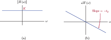
Magnitude and phase characteristics of the system function are
and
A distortion-free system has a magnitude that is constant, and a phase that is a linear function of frequency as shown in Fig. 10.3.
Example 10.1: Distortion caused by the RC circuit
Consider again the simple RC circuit that was used in several examples in Chapters 2, 4 and 7.
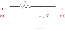
In some cases the RC circuit can be used as a simple model for a wired electrical connection between two points. Such a model would provide a reasonably good approximation to the characteristics of the wired connection provided that the distance between the two points being connected is not too long. (For long distance connections the resistance and the capacitance would have to be modeled as distributed parameters rather than being concentrated at one point each.) The system function for the RC circuit is
Clearly this is not a distortionless system as defined by Eqn. (10.15), however, under certain circumstances it can be considered near distortion-free. The magnitude of the system function is
with the 3-dB cutoff frequency defined as
This magnitude characteristic is shown in Fig. 10.5(a). The phase of the system function is

Magnitude and phase characterictics of the RC circuit of Example 10.1 at low frequencies.
and the corresponding time delay is
The phase characteristic is shown in Fig. 10.5(b).
The magnitude characteristic of the system seems to be relatively flat for frequencies in the vicinity of ω = 0. Similarly, the phase characteristic is close to a straight line, and the time delay is relatively constant for low frequencies. Thus, if we limit the use of the system to input signals that contain only the frequencies ω < < ωc, we could consider the system as near distortion-free.
What is the frequency range (in terms of ωc) in which one can consider the RC circuit approximately distortionless? Of course, the answer depends on the amount of variation in magnitude and/or time delay that we consider negligible. Since both the magnitude and the time-delay characteristics exhibit their peak values at ω = 0, and both are symmetric around that point, we could simply look for a frequency at which the characteristic drops down by a certain percentage. Let ω0 be the frequency at which the magnitude of the system function drops below the peak value by p percent. Using Eqn. (10.18) and realizing that the maximum magnitude is H (0) = 1, we can write
Solving this inequality for ω0 yields
For the frequencies |ω| ≤ 0.1425 ωc, the variation in the magnitude of the system function will be 1 percent or less. If we are willing to tolerate up to 5 percent magnitude variation, then the usable frequency range is |ω| ≤ 0.3287 ωc.
Next consider the phase characteristic given by Eqn. (10.20). Differentiating it with respect to frequency, we obtain
and the slope of the phase characteristic at frequency ω = 0 is
The line that is tangent to the phase characteristic at the frequency ω = 0 is also shown in Fig. 10.5(b) for comparison. The phase remains fairly close to the tangent line for low frequencies. Similar analysis can be performed for the time-delay characteristic of the system; however, because of the form of Eqn. (10.21), arriving at an analytical result is tedious. Instead of trying to duplicate the methodology used in Eqns. (10.22) and (10.23), let us just take the frequency ranges obtained for specified magnitude variations above, and determine the corresponding variation in time delay. It can easily be shown that
If we accept 1 percent variation in magnitude, the corresponding variation in time delay is 0.67 percent. For a 5 percent magnitude variation, the time delay varies by 3.38 percent.
ex_10_1.m
Interactive Demo: dist_demo.m
The demo program “dist_demo” is modeled after Example 10.1 and Fig. 10.5. Magnitude, phase and time-delay characteristics of the RC circuit are graphed. Circuit parameters may be varied using slider controls. Allowed deviation of the magnitude response from a constant value is also specified. A dashed rectangle showing the deviation from ideal behavior is shown on each graph. Zoom-in feature may be used on each graph to get a closer look at the critical values.
- Begin with R = 1 MΩ and C = 1 μF. Let the tolerance limit be 1 percent. Observe the frequency range in which the magnitude stays within 1 percent of the dc value. Also observe deviations from ideal behavior for the phase and the time delay, and compare them to theoretical values.
- Gradually reduce the value of R down to 0.5 MΩ and observe the changes in the frequency range.
- While keeping R = 0.5 MΩ increase the tolerance limit to 2, 3, 4 and 5 percent, and observe the changes in the frequency interval.
Software resources:
dist_demo.m
10.3 Ideal Filters
The conditions for a CTLTI system to be distortionless were identified in Eqns. (10.16) and (10.17) of the previous section, and were graphically illustrated in Fig. 10.3. We observe that, in order to be truly distortionless, a system must have infinite bandwidth. In other words, it must be able to respond to signals containing an infinite range of frequencies. No physically realizable system is capable of doing this.
Furthermore, signals encountered in engineering applications have limited bandwidth, that is, they contain a limited range of frequencies. Consider such a signal x (t). A CTLTI system that satisfies Eqns. (10.16) and (10.17) not necessarily at every frequency, but at all frequencies contained in the signal x (t), would still facilitate distortionless transmission of this signal. Ideal frequency-selective filters are systems that allow distortionless transmission of signal components in a particular frequency range while eliminating all other signal components.
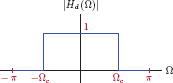
One type is an ideal lowpass filter that is characterized by the system function
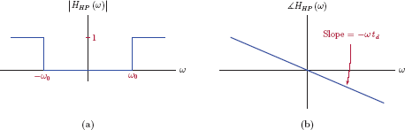
Any signal that contains only the frequencies in the range |ω| ≤ ω0 is transmitted through this system without any distortion of its magnitude or phase characteristics. The magnitude and the phase of the system function HLP (ω) of an ideal lowpass filter are graphed in Fig. 10.6.
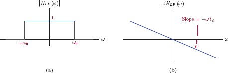
The magnitude of the system function is constant for frequencies in the range −ω0 ≤ ω ≤ ω0. The phase of the system function is a straight line that passes through the origin, with the slope −ωtd. Signals that do not contain any frequencies outside the range |ω| ≤ ω0 would be transmitted through this system without experiencing any distortion. The frequency ω0 in Eqn. (10.29) is the cutoff frequency of the ideal lowpass filter. The parameter td indicates the time delay caused by the filter.
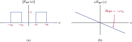
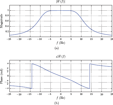
Some signals are bandpass in nature, that is, they contain frequencies in a bandpass frequency range ω1 ≤ |ω| < ω2. Examples of these signals are encountered often in the study of communication systems. The system function of an ideal bandpass filter that would allow distortionless transmission of the appropriate bandpass signal is given by
and is illustrated in Fig. 10.7.
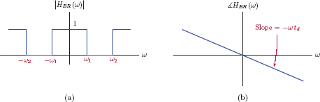
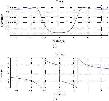
Similarly, ideal highpass and band-reject filters can also be defined. An ideal highpass filter transmits, without distortion, signals that contain only frequencies greater than a minimum value, that is, |ω| ≥ ω0. An ideal band-reject filter, on the other hand, facilitates distortionless transmission of signals that contain only those frequencies that are outside a specified range. Frequencies that satisfy either |ω| ≤ ω1 or |ω| ≥ ω2 are transmitted; all other frequencies are suppressed. Figs. 10.8 and 10.9 illustrate the system functions of ideal highpass and band-reject filters respectively.
The ideal filters discussed above are not practically realizable. In order to see why this is the case, let us determine the impulse response of an ideal filter. For the ideal lowpass filter of Eqn. (10.29), the impulse response can be easily computed from the system function through inverse Fourier transform. Using the inverse Fourier transform relationship given by Eqn. (4.126) on the ideal lowpass filter system function in Eqn. (10.29) we obtain
For convenience, let us express hLP (t) using f0 instead of ω0:
The resulting impulse response is shown in Fig. 10.10.

A few observations are in order regarding the impulse response of the ideal lowpass filter:
- The impulse response hLP (t) given by Eqn. (10.32) is in the form of a sinc function with a peak amplitude of 2f0. This peak occurs at the time instant t = td.
- The zero crossings of the impulse response are uniformly spaced. Consecutive zero crossings are 1/(2f0) apart from each other.
- The impulse response exists for all time instants including t < 0. Thus, the ideal lowpass filter is a non-causal system, and is therefore physically unrealizable.
- Furthermore, no amount of additional time delay would make the impulse response in Eqn. (10.32) causal.
It is also interesting and instructive to derive the impulse response of an ideal bandpass filter the spectrum of which is shown in Fig. 10.7. We could compute the impulse response as the inverse Fourier transform of the system function in Eqn. (10.30), using the approach that was employed in finding the impulse response of the ideal lowpass filter. Instead we will take a simpler approach and express the ideal bandpass filter spectrum in terms of frequency shifts applied to the ideal lowpass filter spectrum. In order to accomplish this, we will initially consider an ideal lowpass filter with zero phase and no time delay, i.e., td = 0. A comparison of Figs. 10.6 and 10.7 reveals that the ideal bandpass filter spectrum with zero phase can be written as
with parameter ωb set to the midpoint frequency of the passband
and the cutoff frequency of the lowpass filter chosen as
The construction of the bandpass filter spectrum from the lowpass filter spectrum is illustrated in Fig. 10.11.
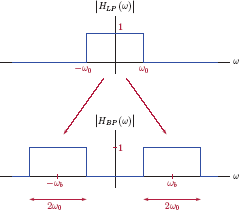
Obtaining the spectrum of the ideal bandpass filter from the spectrum of the ideal lowpass filter.
Using the frequency-shifting property of the Fourier transform, we are now ready to write the impulse response of the ideal bandpass filter as
For convenience we have used frequencies in Hertz rather than the radian frequencies in Eqn. (10.36). This impulse response is for an ideal bandpass filter with no time delay. It may be generalized by adding a linear phase term and the corresponding constant time delay to obtain
Finally, by substituting Eqns. (10.34) and (10.35) into Eqn. (10.37) we get
which is shown graphically in Fig. 10.12.

Interactive Demo: ilpf_demo.m
The demo program “ilpf_demo1.m” illustrates the impulse response of the ideal lowpass filter as defined in Eqn. (10.32), and shown in Fig. 10.10. The magnitude and the phase of the filter transfer function HLP (f) are displayed along with the impulse response hLP (t). The cutoff frequency f0 and the time delay td may be varied using slider controls.
- With the time delay set to td = 0 vary the cutoff frequency and observe its effects on the impulse response.
- With the cutoff frequency fixed at f0 = 100 Hz vary the time delay and observe its effects on the impulse response.
Software resources:
ilpf_demo.m
Interactive Demo: ibpf_demo.m
This demo program illustrates the impulse response of the ideal bandpass filter the system function of which was described by Eqn. (10.38) and Fig. 10.12. The magnitude and the phase of the filter transfer function HBP (f) are displayed along with the impulse response hBP (t). Slider controls allow adjustments to parameters f0 and fb as defined by Eqns. (10.34) and (10.35).
- With the time delay set to td = 0 and fb = 100 Hz vary f0 and observe its effects on the impulse response.
- With td = 0 and f0 = 200 Hz vary fb and observe its effects on the impulse response.
- With f0 = 100 Hz and fb = 150 Hz vary the time delay and observe its effects on the impulse response.
Software resources:
ibpf_demo.m
10.4 Design of Analog Filters
In this section we will focus on designing analog filters to meet a set of user specifications. We have seen in Section 10.3 that filters with ideal characteristics are not realizable since they are non-causal. In practical applications of filtering we seek realizable approximations to ideal filter behavior. The requirements on the frequency spectrum of the filter must be relaxed in order to obtain realizable filters.
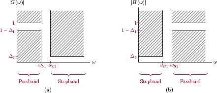
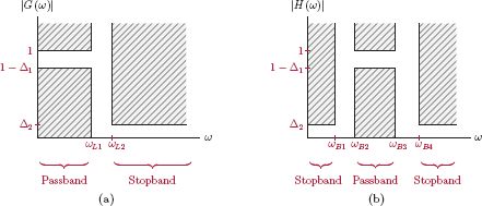
In the design of analog filters, specifications for the desired filter are usually given in terms of a set of tolerance limits for the magnitude response |H (ω)|. Specification diagrams for the four frequency-selective filter types, namely lowpass, highpass, bandpass and band-reject filters, are shown in Fig. 10.13.

Specification diagrams for frequency selective filters: (a) lowpass, (b) highpass, (c) bandpass, (d) band-reject.
Consider the lowpass filter specifications illustrated by Fig. 10.13(a). The frequency interval 0 < ω < ω1 is referred to as the passband of the filter. Within the passband the magnitude of the filter spectrum is required to remain in the range 1 − Δ1 ≤ |H (ω) ≤ 1. For frequencies greater than ω2, that is, in the stopband of the filter, the magnitude is required to stay below Δ2. The parameters Δ1 and Δ2 are called the passband tolerance and the stopband tolerance respectively.
The frequency range ω1 < ω < ω2 between the passband and the stopband is referred to as the transition band where there are no constraints on the magnitude behavior of the filter. The inclusion of a transition band along with the tolerance limits on passband and stopband behavior should allow us to come up with practically realizable designs. It should be noted that the impulse response h (t) is required to be real-valued. Recall from the discussion in Section 4.3.5 of Chapter 4 that if the impulse response is real then the system function is conjugate symmetric, and therefore the magnitude of the system function is an even function of ω. This is the reason why the specification diagrams in Fig. 10.13 display only the positive frequencies.
Specifications for a highpass filter, shown in Fig. 10.13(b) mirror those of the lowpass filter. Bandpass and band-reject filter specifications, shown in Fig. 10.13(c),(d) have two transition bands each.
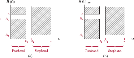
Tolerance limits for a desired filter can also be given on a decibel (dB) scale as shown in Fig. 10.14.

The maximum value of the magnitude response is set as 0 dB. The maximum allowed dB passband ripple Rp and the minimum required dB stopband attenuation As are related to the parameters Δ1 and Δ2 as
and
Given the specifications of the desired filter in the form of one of the specification diagrams in Fig. 10.13, the design problem can be stated as follows:
Analog filter design problem:
Find the system function H (s) of a filter the magnitude response of which remains in the allowed area of the specification diagram.
In general, the analog filter design problem begins with the design of a lowpass prototype filter regardless of the type of filter that is ultimately needed. If a highpass, bandpass or band-reject filter is desired, it is obtained subsequently by means of a frequency transformation to be applied to the lowpass prototype filter. This approach is motivated by the availability of well established methods for the design of analog lowpass filters.
A number of approximation formulas exist in the literature for specifying the squared-magnitude of a realizable lowpass filter spectrum. Some of the better known formulas will be mentioned here.
Butterworth lowpass filters are characterized by the squared-magnitude function
where the parameters N and ωc are the filter-order and the cutoff frequency respectively.
As an alternative to the Butterworth approximation formula, the Chebyshev type-I approximation formula for the squared-magnitude function of a lowpass filter is
where ε is a positive constant. The frequency ω1 is the passband edge frequency. The function CN (ν) in the denominator represents the Chebyshev polynomial of order N.
Chebyshev type-II approximation formula for the squared-magnitude function is similar to the Chebyshev type-I formula.
The parameter ω2 is the stopband edge frequency.
Finally, an elliptic lowpass filter is characterized by the squared-magnitude function
The parameter ε is a positive constant. The function φN (ν) is called a Chebyshev rational function, and is defined in terms of Jacobi elliptic functions.
In the rest of this section we will provide a brief introduction to analog filter design methods. A thorough treatment of analog filter design would be well beyond the scope of this text. There are a number of excellent texts on the subject.
10.4.1 Butterworth lowpass filters
Consider again the Butterworth squared-magnitude function given by Eqn. (10.41). At the frequency ω = ωc the magnitude is equal to . Since this approximately corresponds to the −3 dB point on a logarithmic scale, the parameter ωc is also referred to as the 3-dB cutoff frequency of the Butterworth filter. Furthermore, it can easily be shown that the first 2N − 1 derivatives of the magnitude spectrum |H (ω)| are equal to zero at ω = 0, that is,
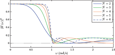
The magnitude characteristic |H (ω)| for a Butterworth filter is said to be maximally flat. Magnitude spectra for Butterworth filters of various orders are shown in Fig. 10.15.

We know that the squared-magnitude function can be expressed as the product of the system function and its complex conjugate, that is
In addition, since the impulse response h (t) of the filter is real-valued, its system function exhibits conjugate symmetry (see Section 4.3.5 of Chapter 4):
Combining Eqns. (10.46) and (10.47) yields
Using the s-domain system function H (s), the problem of designing a Butterworth filter can be stated as follows: Given the values of the two filter parameters ωc and N, find the s-domain system function H (s) for which the squared-magnitude of the function H (ω) matches the right side of Eqn. (10.41).
For a system function H (s) with real coefficients, it can be shown that
The procedure in Eqn. (10.49) needs to be reversed to find the system function H (s). Substituting s for jω, or equivalently, −s2 for ω2 in Eqn. (10.41) we obtain
If H (s) has a pole in the left half s-plane at p1 = σ1 + jω1, then H (−s) has a corresponding pole at . Thus the poles of H (s) are mirror images of the poles of H (−s) with respect to the origin. In order to extract H (s) from the product H (s) H (−s), we need to find the poles of this product, and separate the two sets of poles that belong to H (s) and H (−s) respectively. The cases of even and odd filter-orders N need to be treated separately.
Case 1: N is odd
The poles of the product H (s) H (−s) are the values of s that satisfy the equation
which can be written in the alternative form
where we have used the fact that ej2πk = 1 for all integer k. Poles of H (s) H (−s) are
A few observations are in order:
- All the poles of the product H (s) H (−s) are located on a circle with radius equal to ωc.
- Furthermore, the poles are equally spaced on the circle, and the angle between any two adjacent poles is π/N radians.
- Since H (s) and H (−s) have only real coefficients, all complex poles appear in conjugate pairs.
Fig. 10.16 depicts the situation for ωc = 2 rad/s, and N = 5.
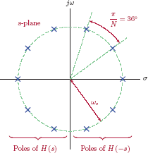
Poles of the product H (s) H (−s) for Butterworth lowpass filter of order N = 5 with 3-dB cutoff frequency ωc = 2 rad/s.
We are interested in obtaining a filter that is both causal and stable. It is therefore necessary to use the poles in the left half of the s-plane for H (s). The remaining poles, the ones in the right half of the s-plane, must be associated with H (−s). The system function H (s) for the Butterworth lowpass filter is constructed in the form
Case 2: N is even
The poles of the product H (s) H (−s) are the solutions of the equation
which can be written as
In this case, the general solution for the poles is
For even filter orders, poles of the magnitude-squared system function are still equally spaced on a circle. Compared to odd filter orders, the only difference in this case is that no poles appear on the real axis. The system function H (s) can be constructed in the same way as it was done for odd values of N.
Poles of H (s) H (−s) for the Butterworth lowpass filter:
Interactive Demo: btw_demo.m
The demo program “btw_demo.m” illustrates the magnitude characteristic of a Butterworth lowpass filter the squared version of which is given by Eqn. (10.41). The desired 3-dB cutoff frequency fc and filter order N may be specified. Observe the following:
- The edges of the magnitude characteristic become sharper as the filter order is increased.
- At the frequency f = fc the magnitude is equal to times its peak value independent of the filter order.
Software resources:
btw_demo.m
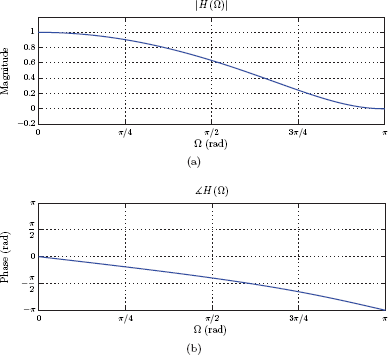
Example 10.2: Butterworth filter design
Determine the system function H (s) of a third-order Butterworth lowpass filter with a 3-dB cutoff frequency of ωc = 20π rad/s.
Solution: Using the Butterworth approximation formula in Eqn. (10.41), the squared-magnitude function of the desired filter can be written as
Substituting ω2 → −s2 in Eqn. (10.58) we obtain
or equivalently
The poles of the function H (s) H (−s) are those values of s that satisfy
Solutions of Eqn. (10.59) are
as shown in Fig. 10.17.

We are particularly interested in the poles that lie in the left half of the s-plane since those are the poles that are associated with H (s). By inspection of Fig. 10.17 it is clear that the poles of H (s) are
We are now ready to construct the transfer function by using these poles:
In order to compute the magnitude and the phase characteristics of the system we need to substitute s = jω into Eqn. (10.59) to obtain
The magnitude of the system function is
and the phase of the system function is
Magnitude and phase responses of the designed filter are shown in Fig. 10.18.
The frequency spectrum of the third-order Butterworth lowpass filter designed in Example 10.2: (a) magnitude, (b) phase.
Software resources:
ex_10_2.m
See MATLAB Exercise 10.1. |
Obtaining N and ωc for the Butterworth lowpass filter
The desired behavior of a lowpass filter to be designed is usually specified in terms of the two critical frequencies ω1 and ω2 as well as the decibel tolerance values Rp and As as shown in Fig. 10.14. The corresponding parameter values for ωc and N need to be determined from the provided set of specifications so that the filter can be designed. If Rp = 3 dB, then we have ωc = ω1. Otherwise the requirements at the two critical frequencies can be expressed as inequalities.
At ω = ω1 we require
Similarly at ω = ω2 we require
Rearranging Eqns. (10.60) and (10.61) yields
and
Dividing both sides of Eqn. (10.62) by the corresponding terms of Eqn. (10.63) we obtain
which can be solved for the filter order N that is needed:
The right side of the inequality in Eqn. (10.65) may or may not be an integer. If it is not, then the value of N needs to be rounded up. The excess tolerance created by rounding N up to the next integer can be used in either the passband or the stopband.
In summary, the parameters of the Butterworth lowpass filter are computed as follows:
Given dB tolerances Rp and As and critical frequencies ω1 and ω2:
10.4.2 Chebyshev lowpass filters
The squared-magnitude function for a Chebyshev lowpass filter is given by
Parameter ε is a positive constant, N is the order of the filter, and ω1 is the passband edge frequency in rad/s (see Fig. 10.13(a)). The term CN (ν) represents the Chebyshev polynomial of order N. Chebyshev filters of this type are sometimes called Chebyshev type-I filters. A variant of the squared-magnitude response in Eqn. (10.66) will be introduced in the next section as the inverse Chebyshev filter or the Chebyshev type-II filter.
Once the values of the parameters ε, N and ω1 are specified, the design procedure proceeds as follows:
- Find CN (ν), the Chebyshev polynomial of order N.
- Substitute ν = ω/ω1 in the polynomial CN (ν).
- Form the Chebyshev type I squared-magnitude function as specified in Eqn. (10.66).
- Find the poles of the system function H (s) from the squared-magnitude function. As in the case of the Butterworth lowpass filter, this involves substituting jω = s into the squared-magnitude function, finding the roots of the denominator polynomial, and separating those poles into two sets, one to be associated with H (s) and the other to be associated with H (s).
Before we carry out the steps outlined above, it will be useful to review the properties of Chebyshev polynomials.
Chebyshev polynomials
The Chebyshev polynomial of order N is defined as
A better approach for understanding the definition in Eqn. (10.67) would be to split it into two equations as
and
The Chebyshev polynomial of a specified order N can be obtained by
- Using trigonometric identities to express cos (Nθ) as a function of cos (θ).
- Replacing each cos (θ) term with ν.
The first two polynomials are easy to obtain from this definition:
To obtain C2 (ν) let us write cos (2θ) in terms of cos (θ) using a trigonometric identity:
Thus, the second-order Chebyshev polynomial is
Higher-order Chebyshev polynomials may be obtained by continuing in this fashion. As the order increases, however, the procedure outlined above becomes increasingly tedious. Fortunately, it is possible to derive a recursive formula to facilitate the derivation of higher-order Chebyshev polynomals.
Let us write cos ((N + 1)θ) and cos((N − 1)θ) using trigonometric identities:
Adding the two equations results in
which can be rearranged to produce the recursive formula we seek:
Thus, the recursive formula for obtaining Chebyshev polynomials is
The recursive formula in Eqn. (10.70) allows any order Chebyshev polynomial to be found provided that the polynomials for the previous two orders are known. With the knowledge of C0 (ν) = 1 and C1 (ν) = ν, the polynomial C2 (ν) can be found as
Similarly C3 (ν) is found as
The behaviors of the first few orders of Chebyshev polynomials are illustrated in Fig. 10.19.

A few interesting characteristics of Chebyshev polynomials can be readily observed:
- All Chebyshev polynomials pass through the point (1, 1), that is, CN (1) = 1 for all N.
- For all Chebyshev polynomials, if |ν| ≤ 1 then |CN (ν)| ≤ 1.
- For |ν| > 1 all Chebyshev polynomials grow monotonically without bound.
- At ν = 0 the behavior of Chebyshev polynomials depends on the order N · CN (0) = 0 if N is odd, and CN (0) = ±1 if N is even.
Fig. 10.20 shows the squared Chebyshev polynomials for the first few orders N.

Squared Chebyshev polynomials oscillate in the amplitude range [0, 1] for |ν| ≤ 1 and N ≥ 2. For |ν| > 1 they grow monotonically without bound.
Software resources: |
See MATLAB Exercise 10.2. |
The squared magnitude function given by Eqn. (10.66) is shown in Fig. 10.21 for several values of N using ε = 0.4 and ω1 = 1 rad/s.

Poles for the Chebyshev lowpass filter
In constructing the system function for a Chebyshev lowpass filter we will use an approach similar to that taken with a Butterworth lowpass filter in Section 10.4.1. First we will determine the poles of the product H (s) H (−s). Recall that the product H (s) H (−s) is obtained by starting with the squared magnitude function |H (ω)|2 and replacing jω with s:
The poles pk of H (s) H (−s) are the solutions of the equation
for k = 0,..., 2N − 1.
Let us define
so that
Using the definition of the Chebyshev polynomial given by Eqn. (10.69) we can rewrite Eqn. (10.74) as
where νk = cos(θk). Solving Eqn. (10.75) for cos (Nθk) yields
Let θk = αk + jβk with αk and βk both as real parameters. Eqn. (10.76) becomes
which, using the appropriate trigonometric identity, can be written as
Recognizing that cos (jN βk) = cosh (Nβk) and sin (jN βk) = j sinh (Nβk), we obtain
Equating real and imaginary parts of both sides of Eqn. (10.79) yields
and
To satisfy Eqn. (10.80) the cosine term must be set equal to zero, leading to
Using this value of αk in Eqn. (10.81) results in
and
The poles of the product H (s) H (−s) can now be determined. Using Eqn. (10.73)
Using the values of αk and βk found, the poles of H (s) H (−s) are
for k = 0,..., 2N − 1. It can be shown that the poles given by Eqn. (10.86) are on an elliptical trajectory. The ones in the left half s-plane are associated with H (s) in order to obtain a causal and stable filter.
Poles of H (s) H (−s) for the Chebyshev type-I lowpass filter:
Interactive Demo: cheb1_demo.m
This demo program illustrates the magnitude response of the Chebyshev type-I lowpass filter, the squared version of which is given by Eqn. (10.42). The cutoff frequency f1, the parameter ε and the filter order N may be specified as desired. Observe the following:
- The edges of the magnitude characteristic become sharper as the filter order is increased.
At the frequency f = f1 the magnitude is equal to
Software resources:
cheb1_demo.m
Example 10.3: Design of a Chebyshev lowpass filter
Design a third-order Chebyshev type-I analog lowpass filter with a passband edge frequency of ω1 = 1 rad/s and ε = 0.4. Afterwards compute and graph the magnitude response of the designed filter.
Solution: Using Eqn. (10.82) the parameter αk is found as
and the parameter βk is obtained from Eqn. (10.84) as
Poles of H (s) H (−s) are found through the use of Eqn. (10.86):
Evaluating Eqn. (10.87) for k = 0,..., 5 yields the following poles:
The first three poles, namely p0, p1 and p2 are in the right half s-plane; therefore they belong to H (−s). The system function H (s) should be constructed using the remaining three poles.
The numerator of H (s) was adjusted to achieve |H (0)| = 0. The magnitude and the phase of H (s) are shown in Fig. 10.22.

The magnitude and the phase of the third-order Chebyshev lowpass filter designed in Example 10.3.
Software resources:
ex_10_3.m
Software resources: |
See MATLAB Exercise 10.3. |
Obtaining N and ε for the Chebyshev lowpass filter
In some design problems it is desired to find the lowest-order filter that satisfies a set of design specifications. The desired behavior of the lowpass filter is typically specified in terms of the two critical frequencies ω1 and ω2 as well as the dB tolerance values Rp and As for the passband and the stopband respectively.
At the frequency ω = ω1 we need
Recall that CN (1) = 1 for all Chebyshev polynomials. Therefore Eqn. (10.88) becomes
which can be solved for ε to yield
In the next step we need to determine the filter order N. At the stopband edge frequency we have the inequality
In order to simplify the notation let us define ω0 = ω2/ω1. Eqn. (10.91 can be expressed as
In the worst case Eqn. (10.92) can be taken with equality and solved for CN (ω0) to yield
in which we have used the value of ε found in Eqn. (10.90). In order to solve Eqn. (10.93) for N we will define some intermediate variables. Let
and
The equation that needs to be solved for N is
Since θ0 is complex (remember that ω0 > 1) we will express it in Cartesian complex form as θ0 = α0 + jβ0, and write (10.96) as
Since F is real, the left side of Eqn. (10.97) must be real as well. Therefore we must have
and
Using Eqn. (10.95) we can write
Solving Eqns. (10.99) and (10.100) for the filter order N we obtain
The value of N obtained through Eqn. (10.101) may not necessarily be an integer, and must be rounded up to the next integer. The excess tolerance obtained by rounding N up causes the stopband inequality given by Eqn. (10.92) to improve. If it is desired to use the excess tolerance for improving the passband response instead, then ε may be recalculated from Eqn. (10.92) using the rounded-up value of N.
In summary, the parameters of a Chebyshev type-I lowpass filter are computed as follows:
Given dB tolerances Rp and As and critical frequencies ω1 and ω2:
Compute ε from one of the following:
Software resources: |
See MATLAB Exercise 10.4. |
10.4.3 Inverse Chebyshev lowpass filters
The squared-magnitude function for an inverse Chebyshev lowpass filter, also referred to as a Chebyshev type-II lowpass filter, is
As in the case of Chebyshev type-I filters, ε is a positive constant and CN (ν) represents the Chebyshev polynomial of order N. The parameter ω2 is the stopband edge frequency (see Fig. 10.13(a)). Magnitude responses of several Chebyshev type-II filters are shown in Fig. 10.23. The magnitude response of the Chebyshev type-II filter is smooth in the passband and has equiripple behavior in the stopband.
Poles and zeros of the inverse Chebyshev filter
The denominator of the squared magnitude function |H (ω)|2 in Eqn. (10.102) is very similar to that of the type-I Chebyshev filter squared magnitude response given by Eqn. (10.66). Consequently, most of the results obtained in the previous section through the derivation of the poles of Chebyshev type-I lowpass filter will be usable. For an inverse Chebyshev filter the poles pk of the product H (s) H (−s) are the solutions of the equation
for k = 0,..., 2N − 1.
Let
so that Eqn. (10.103) becomes
This result is identical to that obtained in Eqn. (10.74) for computing the poles of the Chebyshev type-I lowpass filter, therefore, the solution obtained for pk may be used here as well. We have
with
and
The poles pk are determined from αk and βk as
As discussed before, the poles in the left half s-plane are associated with H (s)in order to obtain a causal and stable filter. The zeros of H (s) H (s) are found by solving
It can be shown that the zeros of the inverse Chebyshev lowpass filter are
where the upper limit K is computed as
A summary of the results is given below:
Poles of H (s) H (−s) for the Chebyshev type-II lowpass filter:
Zeros of H (s) for the Chebyshev type-II lowpass filter:
The upper limit K is computed as
Interactive Demo: cheb2_demo.m
This demo program illustrates the magnitude response of the Chebyshev type-II lowpass filter, the squared version of which is given by Eqn. (10.43). The stopband edge frequency f2, the parameter and the filter order N may be specified as desired. Observe the following:
- The edges of the magnitude characteristic become sharper as the filter order is increased.
At the frequency f = f2 the magnitude is equal to
cheb2_demo.m
Software resources: |
See MATLAB Exercise 10.5. |
Obtaining N and ε for the inverse Chebyshev lowpass filter
The inverse Chebyshev lowpass filter is uniquely described by the choice of parameters ω2, ε and N. If the desired filter is described by the specification diagram of Fig. 10.14 then we have the set of parameters Rp, As, ω1 and ω2 from which ε and N must be determined.
The first step is to choose the parameter ε so that the magnitude response of the filter fills the allowed area completely in the stopband.
Evaluating the squared magnitude response given by Eqn. (10.102) at the stopband edge frequency ω = ω2 and remembering that CN (1) = 1 for all Chebyshev polynomials we obtain
which can be solved for ε to yield
Next the filter order N needs to be determined. At the passband edge frequency we have the following inequality:
Let us define ω0 = ω2/ω1 to simplify the notation. Eqn. (10.115) can be written as
In the worst case Eqn. (10.116) can be taken with equality and solved for CN (ω0) to yield
after the substitution of the result found in Eqn. (10.114). Incidentally this is identical to Eqn. (10.93); therefore, its solution must be identical as well. Using the definition of parameter F as given by Eqn. (10.94) the minimum filter order that satisfies the specifications is found as
If Eqn. (10.118) does not yield an integer, it must be rounded up to the next integer. The excess tolerance created by the rounding up of N can be used in either frequency band by solving Eqn. (10.113) or Eqn. (10.116) for ε.
In summary, the parameters of a Chebyshev type-II lowpass filter are computed as follows:
Given dB tolerances Rp and As and critical frequencies ω1 and ω2:
Compute ε from one of the following:
10.4.4 Analog filter transformations
In preceding sections we have discussed the design of analog lowpass filters. Design formulas for Butterworth, Chebyshev and elliptic squared-magnitude functions were presented only for lowpass filters. If a different filter type such as a highpass, bandpass or band-reject filter is needed, it is obtained from a lowpass filter by means of an analog filter transformation.
Let G (s) be the system function of an analog lowpass filter, and let H (λ) represent the new filter to be obtained from it. For the new filter we use λ as the Laplace transform variable. H (λ) is obtained from G (s) through a transformation such that
The function s = f (λ) is the transformation that converts the lowpass filter into the type of filter desired.
Lowpass to highpass transformation
Consider the specification diagrams shown in Fig. 10.24 for a lowpass filter with magnitude response |G (ω)| and a highpass filter with magnitude response |H (ω)|.
It is desired to obtain the highpass filter system function H (λ) from the lowpass filter system function G (s). The transformation
can be used for this purpose The magnitudes of the two filters are identical at their respective passband edge frequencies, that is,
The stopband edges of the two filters are related by
so that we have
Example 10.4: Design of a Chebyshev highpass filter
Recall that a third-order Chebyshev type-I analog lowpass filter was designed in Example 10.3 with a cutoff frequency of ω1 = 1 rad/s and ε = 0.4. The system function of the filter was found to be
Convert this filter to a highpass filter with a critical frequency of ωH2 = 3 rad/s. Afterwards compute and graph the magnitude response of the designed filter.
Solution: The critical frequency of the lowpass filter is ωL1 = 1 rad/s; therefore, we will use the transformation
which leads to the system function
The magnitude and the phase of H (λ) are shown in Fig. 10.25.
The magnitude and the phase of the third-order Chebyshev highpass filter designed in Example 10.4.
Software resources:
ex_10_4.m
Software resources: |
See MATLAB Exercise 10.6. |
Lowpass to bandpass transformation
Specification diagrams in Fig. 10.26 show a lowpass filter with magnitude response |G (ω)| and a bandpass filter with magnitude response |H (ω)|.
It is desired to obtain the bandpass filter system function H (λ) from the lowpass filter system function G (s). The transformation
can be used for this purpose. We require
and
It can be shown that (see Problem 10.10) these requirements are met if the parameters ω 0 and B are chosen as
The parameter ω0 is the geometric mean of the passband edge frequencies of the bandpass filter. The parameter B is the ratio of the bandwidth of the bandpass filter to the bandwidth of the lowpass filter.
Lowpass to band-reject transformation
Specification diagrams in Fig. 10.27 show a lowpass filter with magnitude response |G (ω)| and a band-reject filter with magnitude response |H (ω)|.
In order to obtain the band-reject filter system function H (λ) from the lowpass filter system function G (s), the transformation to be used is in the form
For a lowpass filter to be converted into a highpass filter we require
and
It can be shown that (see Problem 10.12) these requirements are met if the parameters ω0 and B are chosen as
See MATLAB Exercise 10.7. |
10.5 Design of Digital Filters
In this section we will briefly discuss the design of discrete-time filters. Discrete-time filters are viewed under two broad categories: infinite impulse response (IIR) filters, and finite impulse response (FIR) filters. The system function of an IIR filter has both poles and zeros. Consequently the impulse response of the filter is of infinite length. It should be noted, however, that the impulse response of a stable IIR filter must also be absolute summable, and must therefore decay over time. In contrast, the behavior of an FIR filter is controlled only by the placement of the zeros of its system function. For causal FIR filters all of the poles are at the origin, and they do not contribute to the magnitude characteristics of the filter.
For a given set of specifications, an IIR filter is generally more efficient than a comparable FIR filter. On the other hand, FIR filters are always stable. Additionally, a linear phase characteristic is possible with FIR filters whereas causal and stable IIR filters cannot have linear phase. The significance of a linear phase characteristic is that the time delay is constant for all frequencies. This is desirable in some applications, and requires the use of an FIR filter.
10.5.1 Design of IIR filters
Consider again the specification diagram for an analog lowpass filter shown in Fig. 10.13(a). It can be adapted for the system function of a discrete-time filter as shown in Fig. 10.28.
The magnitude specifications of the discrete-time filter are given in the angular frequency range 0 ≤ Ω < π. Since the impulse response of the filter to be designed is real, the magnitude is an even function of Ω, and therefore the part of the magnitude response in the range −π ≤ Ω < 0 is obtained as the mirror image of what is shown in Fig. 10.28. Furthermore, the magnitude response is 2π-periodic.
Specification diagrams for other filter types (highpass, bandpass or band-reject) can be adapted to discrete-time filters in a similar manner.
The most common method of designing IIR filters is to start with an appropriate analog filter, and to convert its system function to the system function of a discrete-time filter by means of some transformation. Designing a discrete-time filter by this approach involves a three step procedure:
- The specifications of the desired discrete-time filter are converted to the specifications of an appropriate analog filter that can be used as a prototype. Let the desired discrete-time filter be specified through critical frequencies Ω1 and Ω2 along with tolerance values Δ1 and Δ2. Analog prototype filter parameters ω1 and ω2 need to be determined. (If the filter type is bandpass or band-reject, two additional frequencies need to be specified.)
- An analog prototype filter that satisfies the design specifications in step 1 is designed. Its system function G (s) is constructed.
- The analog prototype filter is converted to a discrete-time filter by means of a transformation. Specifically, a z-domain system function H (z) is obtained from the analog prototype system function G (s). The designed discrete-time filter can be analyzed using the techniques discussed in Chapters 5 and 8, and implemented using the block diagram methods discussed in Chapter 8.
Step 2 of the design procedure, namely the design of an analog prototype, was discussed in Section 10.4. The problem of converting an analog system function to a discrete-time system function (step 3) will be discussed next, followed by the conversion of specifications (step 1). The reason for this particular order is because step 1 is dependent on which method is to be used in step 3.
Analog to discrete-time conversion
Step 3 of the design procedure discussed above requires a discrete-time system function to be obtained from the analog system function. The goal is to come up with a system function H (z) the characteristics of which resemble those of the analog system function G (s) in some way. The goal is somewhat loosely defined; there is no clear definition of when two filters resemble each other. There is also the question of which characteristics of the two filters (magnitude, phase, time-delay, impulse response, etc.) exhibit similarity. In most cases analog prototype filters are designed based on their magnitude responses. Therefore, our goal will be to obtain a reasonable degree of similarity between the magnitude characteristics of the two filters.
The main challenge is the fact that the system function H (Ω) is 2π-periodic whereas the analog prototype filter system function G (ω) is not. Consequently, an exact match between the system functions is not possible. Multiple methods exist for obtaining an approximate match. Two of these methods, namely impulse invariance and bilinear transformation, will be discussed in the remainder of this section.
Impulse invariance
A possible method of obtaining a discrete-time filter from an analog prototype is to ensure that the impulse response is preserved in the conversion process. Specifically, the discrete-time filter is chosen such that its impulse response is equal to a scaled and sampled version of the impulse response of the analog prototype:
The relationship in Eqn. (10.132) is the sampling relationship discussed in Chapter 6. The reason for the scale factor T will become obvious when we consider the magnitude spectrum of the resulting discrete-time filter.
Let the system function for a causal analog prototype filter be G (s) which can be expanded into partial fractions in the form
where pi are the poles, and ki are the corresponding residues. The impulse response is
Under impulse-invariant design the impulse response of the discrete-time system is required to be
The system function of the discrete-time filter is found by taking the z transform of h [n] as
Comparing Eqns. (10.133) and (10.136) we conclude that H (z) can be obtained directly from the partial fraction expansion of G (z) without the intermediate steps of computing g (t) and sampling it.
An important issue in the conversion of an analog filter to a discrete-time filter is the requirement that a stable discrete-time filter be obtained from a stable analog filter. The poles of the analog prototype filter are at
The corresponding poles of the discrete-time filter obtained through impulse invariance are at
For a casual and stable analog prototype filter the poles are in the left half s-plane, and therefore σi < 0 for i = 1,..., N. This implies that
We are assured that a casual and stable analog prototype filter leads to a casual and stable discrete-time filter when the impulse invariance technique is used.
Finally we need to understand the relationship between the magnitude responses of the analog prototype filter and the resulting discrete-time filter. This step is easy owing to the sampling relationship between g (t) and h [n] given by Eqn. (10.132). Using Eqn. (6.25) from Chapter 6 we obtain
In order to avoid aliasing, the analog prototype filter must be bandlimited such that
and the spectrum of the resulting discrete-time filter is a frequency-scaled version of the analog prototype filter spectrum in the range −π ≤ < ω < π. Nevertheless, the bandlimiting condition given by Eqn. (10.141) is often not satisfied by the analog prototype filter (none of the analog designs considered in Section 10.4 are perfectly bandlimited). Therefore, the spectrum of the resulting discrete-time filter is an aliased version of the spectrum of the analog prototype. This is illustrated in Fig. 10.29.

Based on Eqn. (10.140) the value of the system function H (Ω) at a specific frequency Ω = Ω0 is determined by contributions from the analog prototype system function G (ω) at frequencies
Due to the aliasing of the spectrum, impulse-invariant designs are only useful for lowpass filters for which aliasing can be kept at acceptable levels.
Interactive Demo: impinv_demo.m
This demo program illustrates the mapping of the jω-axis of the s-plane to the unit circle of the z-plane for impulse invariant design. Magnitude response of an analog prototype filter with system function
is shown along with the magnitude response of discrete-time filter derived from it using the impulse invariance technique. The sampling interval T may be specified using a slider control. For a selected value of Ω, the values of ω at which the analog prototype contributes to the discrete-time filter are shown.
Software resources:
impinv_demo.m
Example 10.5: Impulse invariant design of a lowpass filter
Consider the third-order Chebyshev type-II analog lowpass filter designed in Example 10.3. Convert this filter to a discrete-time filter using the impulse invariance technique with T = 0.2 s. Afterwards compute and graph the magnitude response of the discrete-time filter.
Solution: The system function of the analog prototype filter designed in Example 10.3 was
which can be written in partial fraction form as
Using Eqn. (10.136) the discrete-time filter system function is written in partial fraction form as
The closed form expression for H (z) is
The magnitude and the phase of H (z) are shown in Fig. 10.30.

The magnitude and the phase of the third-order Chebyshev lowpass IIR filter designed in Example 10.5.
Note that aliasing can be kept at a negligible level with the choice of T, and the analog frequency ω1 = 1 rad/s corresponds to the discrete-time frequency Ω = 0.2 radians.
Software resources:
ex_10_5a.m
ex_10_5b.m
See MATLAB Exercise 10.8. |
Example 10.5 demonstrates that, if the analog prototype filter system function G (s) is fixed, then the sampling interval should be chosen as small as possible to minimize the effect of aliasing. However, a typical IIR filter design problem begins with the critical frequencies Ω1 and Ω2 of the discrete-time filter. Let the corresponding critical frequencies of the analog prototype filter to be designed be ω1 and ω2 respectively. Recall from the sampling relationship that the analog frequencies and the discrete-time frequencies are related by ω = Ω/T. If the sampling interval is T, the sampling rate is ωs = 2π/T, and we obtain
and
For specified discrete-time critical frequencies, increasing the sampling rate ωs does not improve the aliasing condition since the bandwidth of the signal g (t) to be sampled also increases proportionally. Therefore the choice of T is irrelevant and we often use T = 1 s for simplicity. Example 10.6 will illustrate this.
Example 10.6: Impulse invariant design specifications
A lowpass IIR filter is to be designed with the following specifications:
Impulse invariance technique is to be used for converting an analog prototype filter to a discrete-time filter. Determine the specifications of the analog prototype if the sampling interval is to be
- T = 1 s
- T = 2 s
Solution:
Using T = 1 s, the critical frequencies of the analog prototype filter are
The dB tolerance limits are unchanged:
Let the system function for the analog prototype filter be G1 (ω) yielding an impulse response g1 (t). The impulse response of the discrete-time filter is
With T = 2 s, the critical frequencies of the analog prototype filter are
The dB tolerance limits are unchanged as before. Let the system function for the analog prototype filter be G2 (ω) so that its impulse response is g2 (t). The impulse response of the discrete-time filter is obtained by sampling g2 (t) every 2 seconds, that is,
We have thus obtained two discrete-time filters with the two choices of the sampling interval T. What is the relationship between these two filters? Let us realize that G1 (0.2π) = G2 (0.1π) and G1 (0.25π) = G2 (0.125π). Generalizing these relationships we have
Based on the scaling property of the Fourier transform (see Section 4.3.5 of Chapter 4) this implies that
and therefore
The two IIR filters designed are identical and independent from the choice of T.
Bilinear transformation
The impulse invariance technique has a severe shortcoming that prevents its adoption as a general method applicable to the design of all filter types. The aliasing effect that results from sampling the impulse response limits its usefulness to lowpass filters only. An alternative technique known as bilinear transformation avoids aliasing and overcomes this limitation.
In order to develop the idea we will work with a first-order system; however, the technique developed will be applicable to higher-order systems as well. Consider a first-order analog prototype filter described by the system function
The differential equation for the filter is
Let us define an intermediate variable ωa (t) as
so that Eqn. (10.147) becomes
Since the goal is to obtain a discrete-time filter, we will write the discrete-time version of Eqn. (10.148) as
where we have defined ω[n] = ωa (nT), y[n] = ya (nT) and x[n] = xa (nT). The equivalent relationship between ya(t) and ωa(t) is
Letting t0 = (n − 1)T and t = nT, a discrete-time approximation to ya (t) can be obtained using the trapezoidal approximation method (see Problem 3.35 at the end of Chapter 3):
Substituting Eqn. (10.149) into Eqn. (10.151) the difference equation between x[n] and y[n] is found as
which can be simplified to
The system function of the corresponding discrete-time filter is obtained from Eqn. (10.153) as
By comparing Eqns. (10.146) and (10.154) we conclude that the transformation between the s-plane and the z-plane is given by
This is referred to as the bilinear transformation. Solving Eqn. (10.155) for z yields
as the inverse of bilinear transformation. Since the relationship between s and z is invertible, bilinear transformation represents a one-to-one mapping between the s-plane and the z-plane. For each point in the s-plane, there is one and only one point in the z-plane, and vice versa. Contrast this with the impulse invariance technique that maps multiple frequencies on the jω-axis of the s-plane to a single point on the unit circle of the z-plane, resulting in aliasing.
In order to understand how the jω-axis of the s-plane is mapped to the z-plane we will evaluate Eqn. (10.156) for s = jω:
The magnitude of the expression is
Since the magnitude of z is equal to unity for all ω, the jω-axis of the s-plane is mapped onto the unit circle of the z-plane. Furthermore, the entire jω-axis of the s-plane is mapped onto the unit circle of the z-plane only once, and there is no aliasing. Bilinear transform does not suffer from the limitations of the impulse invariance technique, and can be used for designing all four frequency-selective filter types. Setting z = ejΩ in Eqn. (10.158) we have
and
Eqn. (10.160) gives the relationship between analog frequencies ω and discrete-time frequencies Ω. It is shown graphically in Fig. 10.31.
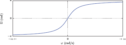
It is evident from Fig. 10.31 that the mapping of frequencies is highly nonlinear. For low frequencies the relationship between ω and Ω is almost linear, however, for high frequencies we see that significant changes in ω trigger minuscule changes in Ω. This behavior is necessary if we want to map an infinite range of analog frequencies to a 2π-radian range of discrete-time frequencies. Fig. 10.32 illustrates the mapping from the jω-axis of the s-plane and the unit circle of the z-plane.

The jω-axis of the s-plane is mapped onto the unit circle of the z-plane. Each point on the jω-axis of the s-plane maps to one and only one point on the unit circle of the z-plane. Furthermore, each point in the left half s-plane maps to one and only one point inside the unit circle of the z-plane. This ensures that a stable analog prototype filter leads to a stable discrete-time filter under bilinear transformation.
Interactive Demo: biln_demo.m
This demo program illustrates the mapping of the jω-axis of the s-plane to the unit circle of the z-plane for bilinear transformation. Magnitude response of an analog prototype filter
is shown along with the magnitude response of discrete-time filter derived from it using bilinear transformation. The sampling interval T may be specified using a slider control. For a selected value of ω, the corresponding value of Ω is shown.
Software resources:
biln_demo.m
Example 10.7: Applying bilinear transformation
A second-order analog filter has the system function
Convert this filter to a discrete-time filter using bilinear transformation with T = 2 s. Afterwards compute and graph the magnitude response of the discrete-time filter.
Solution: Substituting
we obtain
which can be simplified to
The magnitude and the phase of H (z) are shown in Fig. 10.33.
Software resources:
ex_10_7.m
Obtaining analog prototype specifications
As discussed earlier, the first step in designing IIR filters is to convert the specifications of the desired discrete-time filter to the corresponding specifications of an appropriate analog prototype filter. For lowpass and highpass filters two edge frequencies Ω1 and Ω2 are given along with the tolerance values Δ1 and Δ2, or their decibel equivalents Rp and As. The critical frequencies for the discrete-time IIR filter must be translated to the critical frequencies of the analog prototype based on which method is to be used in step 3 of the design process. If impulse invariance will be used in converting the analog prototype to a discrete-time filter, critical frequencies of the analog prototype are computed as
since the conversion process is based on sampling the impulse response of the analog prototype filter. If, on the other hand, bilinear transformation is to be used, then the distortion of the frequency axis must be taken into account. In this case the critical frequencies for the analog prototype filter are computed as
This is called prewarping. Recall that, when bilinear transformation is applied to the analog prototype filter in step 3 of the design process, the frequency axis is distorted as described by Eqn. (10.160). Prewarping counteracts this distortion at the critical frequencies.
Example 10.8: IIR filter design using bilinear transformation
Using bilinear transformation design a Butterworth lowpass filter with the following specifications:
Solution: We will use T = 1 s. The critical frequencies of the analog prototype filter are found using the prewarping equation applied to Ω1 and Ω2:
Next the filter order N needs to be determined using Eqn. (10.65).
The filter order needs to be chosen as N = 4. The 3-dB cutoff frequency is found by setting the magnitude at the stopband edge to −As dB by solving
so that
which yields ωc = 0.7146 rad/s. The analog prototype filter can now be designed using Butterworth lowpass filter design technique described in Section 10.4.1 with the values of N and ωc found. The system function is
The system function for the discrete-time filter is found through bilinear transformation using the replacement
which results in
The dB magnitude of the resulting filter is shown in Fig. 10.34 with the tolerance limits.

Software resources:
ex_10_8a.m
ex_10_8b.m
Software resources: |
See MATLAB Exercises 10.9, 10.10, and 10.11. |
10.5.2 Design of FIR filters
A length-N FIR filter is completely characterized by its finite-length impulse response h[n] for n =0,...,N − 1. The system function for such a filter is computed as
The system function can also be written using non-negative powers of z in the form
which leads us to the following conclusions:
- Length-N FIR filter has a system function that is of order N − 1.
- The system function H (z) has N − 1 zeros and as many poles.
- The placement of zeros of the filter is determined by the sample amplitudes of the impulse response h[n].
- In contrast, all poles of the length-N FIR filter are at the origin, independent of the impulse response. Therefore, FIR filters are inherently stable.
- The magnitude response of the filter is determined only by the locations of the zeros since the poles at the origin do not contribute to the magnitude response (see Section 8.5.4).
The sample amplitudes of the impulse response h[n] for n = 0,...,N − 1 are often referred to as the filter coefficients. In this section we will present two approaches to the problem of designing FIR filters: one very simplistic approach that is nevertheless instructive, and one elegant approach that is based on computer optimization. In a general sense, the design procedure for FIR filters consists of the following steps:
- Start with the desired frequency response. Select the appropriate length N of the filter. This choice may be an educated guess, or may rely on empirical formulas.
- Choose a design method that attempts to minimize, in some way, the difference between the desired frequency response and the actual frequency response that results.
- Determine the filter coefficients h[n] using the design method chosen.
- Compute the system function and decide if it is satisfactory. If not, repeat the process with a different value of N and/or a different design method.
It was discussed earlier in this chapter that one of the main reasons for preferring FIR filters over IIR filters is the possibility of a linear phase characteristic. Linear phase is desirable since it leads to a time-delay characteristic that is constant independent of frequency. As far as real-time implementations of IIR and FIR filters are concerned, we have seen that IIR filters are mathematically more efficient and computationally less demanding of hardware resources compared to FIR filters. If linear phase is not a significant concern in a particular application, then an IIR filter may be preferred. If linear phase is a requirement, on the other hand, an FIR filter must be chosen even though its implementation may be more costly. Therefore, in the discussion of FIR design we will focus on linear-phase FIR filters.
Conditions for linear phase
It can be shown that a length-N FIR filter with impulse response h[n] has a linear phase characteristic if
where the upper limit K is set as follows:
The condition given by Eqns. (10.166) and (10.167) leads to four possible scenarios:
- N : even, and h[n] = h[N − 1 − n] for N = 0,...,N/2 − 1
- N : even, and h[n] = −h[N − 1 − n] for N = 0,...,N/2 − 1
- N : odd, and h[n] = h[N − 1 − n] for N = 0,..., (N − 1)/2
- N : odd, and h[n] = −h[N − 1 − n] for N = 0,..., (N − 1)/2
In addition, it can be shown that the constant time delay for a length-N linear-phase FIR filter is
for all four possibilities. It is interesting to see that the time-delay nd is not an integer when N is even.
A complete proof of linear-phase conditions must address each of the four possibilities listed above (see Problems 10.17 and 10.19).
Example 10.9: Phase of FIR filter with symmetric impulse response
A length-5 FIR filter has the impulse response
Show that the phase characteristic of H (Ω) is a linear function of Ω.
Solution: The DTFT of the impulse response is
Let us factor out e−j2Ω and write the result as
The expression in square brackets contains symmetric exponentials. Using Euler’s formula, it becomes
which is purely real. Using Eqn. (10.170) in Eqn. (10.169) we obtain
The phase response of the filter is
corresponding to a time delay of nd = 2 samples. The magnitude and the phase of the system function are shown in Fig. 10.35.

It should be noted that the phase characteristic is linear in spite of the vertical jumps in Fig. 10.35(b). These vertical sections are due to the fact that A (Ω) is negative for some frequencies. Therefore, the magnitude |H (Ω)| is
and the phase is
What matters for linear phase is that all non-vertical sections of the phase characteristic have the same slope value.
Software resources:
ex_10_9.m
We are now ready to discuss FIR filter design. First the Fourier series design method will be discussed. The use of window functions to overcome the fundamental problems encountered will be explored. Afterwards we will briefly discuss the Parks McClellan technique.
Fourier series design of FIR filters
An ideal lowpass discrete-time filter with a cutoff frequency Ωc has the system function
as shown in Fig. 10.36. The filter has zero phase and zero time delay.
The impulse response of the ideal discrete-time lowpass filter is found by taking the inverse DTFT of Hd (Ω) given by Eqn. (10.171).
The result in Eqn. (10.172) is shown in Fig. 10.37 for Ωc = 0.4π.

The result obtained in Eqn. (10.172) for hd[n] is valid for all N. Therefore, hd[n] infinitely long, and cannot be the impulse response of an FIR filter. On the other hand, sample amplitudes of hd[n] get smaller as the sample index is increased in both directions. A finite-length impulse response can be obtained by truncating hd[n] as follows:
The truncated impulse response has 2M + 1 samples for n = −M,...,M. Truncation of the ideal impulse response causes the spectrum of the filter to deviate from the ideal spectrum. The system function for the resulting filter is
An example is shown in Fig. 10.38. The truncated impulse response with M = 11 is shown in Fig. 10.38(a), and the magnitude spectrum of the resulting length-23 filter is shown in Fig. 10.38(b).
![Figure showing (a) The truncated impulse response hd[n] for M = 11, and (b) its magnitude spectrum.](http://imgdetail.ebookreading.net/data/1/9781466598546/9781466598546__signals-and-systems__9781466598546__image__975x002.png)
The truncated impulse response hT[n] is still non-causal owing to the fact that the filter has zero phase. In order to obtain a causal filter, a delay of M samples must be incorporated into the impulse response, resulting in
Thus, h[n] corresponds to a causal FIR filter. Using the time shifting property of the DTFT (see Section 5.3.5 of Chapter 5), the system function H (Ω) of the causal filter is related to HT (Ω) by
The addition of the M-sample delay only affects the phase of the system function and not its magnitude. Since h[n] is both causal and finite-length, it is the impulse response of a valid FIR filter.
It is worth observing that the impulse response hd[n] given by Eqn. (10.172) is an even function of n. Even symmetry is preserved in hT[n] obtained in Eqn. (10.173) by truncating hd[n]. Finally, when h[n] is obtained by time shifting hT[n] by M samples, the symmetry necessary for linear phase is preserved. Therefore, any filter designed using this technique will have linear phase.
Example 10.10: Fourier series design
Using the Fourier series method, design a length-15 FIR lowpass filter to approximate an ideal lowpass filter with Ωc = 0.3π rad.
Solution: The impulse response of the ideal lowpass filter is
Since N = 2M + 1 = 15 we have M = 7. The truncated impulse response is
The impulse response of the FIR filter is
which can be evaluated as
The magnitude response of the designed filter is shown in Fig. 10.39.

ex_10_10a.m
ex_10_10b.m
A by-product of truncating the impulse response in Eqn. (10.173) is the oscillatory behavior of the frequency response that is particularly evident around the cutoff frequency Ωc. This effect was observed as the Gibbs phenomenon in earlier chapters. An alternative way of expressing the truncation of hd[n] given by Eqn. (10.173) is
where ω[n] is a rectangular window function defined as
Based on the multiplication property of the DTFT (see Section 5.3.5 of Chapter 5), the spectrum of hT[n] is the convolution of the spectra of hd[n] and ω[n].
which is illustrated in Fig. 10.40.
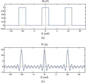
As the spectra in Fig. 10.40 reveal, the reason behind the oscillatory behavior of HT (Ω) especially around Ω = Ωc is the shape of the spectrum W (Ω). The high-frequency content of W (Ω), on the other hand, is mainly due to the abrupt transition of the rectangular window from unit amplitude to zero amplitude at its two edges. The solution is to use an alternative window function in Eqn. (10.177), one that smoothly tapers down to zero at its edges, in place of the rectangular window. The chosen window function must also be an even function of n in order to keep the symmetry of hT[n] for linear phase. A large number of window functions exist in the literature. A few of them are listed below:
Triangular (Bartlett) window:
Hamming window:
Hanning window:
Blackman window:
The four window functions listed are shown in Fig. 10.41 for M = 12.

Window functions: (a) triangular (Bartlett) window, (b) Hamming window, (c) Hanning window, (d) Blackman window.
Fig 10.42 shows the decibel magnitude spectra for rectangular, Hamming and Blackman windows for comparison.
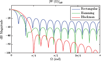
It is seen that the rectangular window has stronger side lobes than the other two window functions. Hamming window provides side lobes that are at least 40 dB below the main lobe, and the side lobes for the Blackman window are at least 60 dB below the main lobe. The downside to side lobe suppression is the widening of the main lobe.
We are now ready to summarize the Fourier series design method for linear-phase FIR filters:
- Determine the ideal impulse response hd[n] as the inverse DTFT of the ideal spectrum being approximated.
- Multiply the ideal impulse response with the selected length-(2M + 1) window function to obtain a finite-length impulse response hT[n] = hd[n] ω[n].
- Obtain the causal FIR impulse response by time shifting hT [n], that is, h[n] = hT [n − M].
Example 10.11: Fourier series design using window functions
Redesign the filter of Example 10.10 using Hamming and Blackman windows.
Solution: Using a window function the truncated impulse response is
and the impulse response of the FIR filter is
For the Hamming window, Eqn. (10.184) yields
When the Blackman window is used, we get
Magnitude responses of the two filters are shown in Fig. 10.43.

Software resources:
ex_10_11a.m
ex_10_11b.m
Filter types other than lowpass
In the discussion above we have concentrated on the design of lowpass FIR filters. Other types of filters can also be designed; the only modification that is needed is in determining the ideal impulse response hd[n]. Expressions for the ideal impulse responses of highpass, bandpass and band-reject filters can be derived from Eqn. (10.172) as follows:
Highpass:
Bandpass:
Band-reject:
Software resources: |
Parks-McClellan technique for FIR filter design
FIR filter design technique due to Parks and McClellan is also referred to as the Remez exchange method. It is based on the idea of finding a polynomial approximation to the desired frequency response by minimizing the largest approximation error.
The Fourier series design method discussed in the previous section, when used with a rectangular window, provides the optimum solution in the sense of mean-squared error. If the error between the desired frequency response and the actual frequency response is E (Ω), then the length-N FIR filter designed using the Fourier series method leads to the mean-squared error
that is the smallest possible with N coefficients. On the other hand, we have seen that the magnitude response of the filter suffers from oscillatory behavior near discontinuities of the spectrum.
Better approximations can be obtained if we minimize the maximum value of the error rather than its mean-squared value. Parks-McClellan algorithm begins with an initial guess of the set of frequencies for the extrema of E (Ω). The locations of the extrema are then iteratively shifted until the maximum deviation from the ideal frequency response is made as small as possible.
Computational details of the Parks-McClellan algorithm are outside the scope of this text and may be found in references. We will provide examples of using MATLAB for designing Parks-McClellan filters in the MATLAB Exercises section.
Software resources: |
10.6 Further Reading
[1] A.V. Oppenheim and R.W. Schafer. Discrete-Time Signal Processing. Prentice Hall, 2010.
[2] R. Schaumann and M.E. Van Valkenburg. Design of Analog Filters. Oxford University Press, 2010.
[3] R.A. Schilling, R.J. Schilling, and P.D. Sandra L. Harris. Fundamentals of Digital Signal Processing Using MATLAB. Cengage Learning, 2010.
[4] L. Tan and J. Jiang. Digital Signal Processing: Fundamentals and Applications. Elsevier Science, 2013.
[5] F. Taylor. Digital Filters: Principles and Applications with MATLAB. IEEE Series on Digital and Mobile Communication. Wiley, 2011.
[6] L.D. Thede. Practical Analog and Digital Filter Design. Artech House, 2005.
[7] L. Wanhammar. Analog Filters Using MATLAB. Springer London, Limited, 2009.
MATLAB Exercises
MATLAB Exercise 10.1: Butterworth analog filter design
MATLAB function butter(..) may be used for designing analog Butterworth filters. For example, a fourth-order Butterworth lowpass filter with a 3-dB cutoff frequency of ωc = 3 rad/s is designed as follows:
>> [num , den] = butter (4 ,3 , ’s’)
num =
0 0 0 0 81.0000
den =
1.0000 7.8394 30.7279 70.5544 81.0000
The third argument ’s’ is needed for specifying that an analog filter is desired since the function butter(..) can be used for designing both analog and discrete-time Butterworth filters. The vectors “num” and “den” returned by the function indicate an s-domain system function
for the designed filter. Magnitude and phase characteristics of the designed filter may be graphed with the following statements:
>> omg = [-10:0.01:10];
>> H = freqs (num ,den , omg);
>> plot (omg , abs (H));
>> plot (omg , angle (H));
Software resources:
matex_10_1a.m
matex_10_1b.m
MATLAB Exercise 10.2: Chebyshev polynomials
In this exercise we will develop and test a function for computing the coefficients of the Chebyshev polynomial of a specified order N. The N-th order Chebyshev polynomial CN (ν) can be computed from the order of the two lower order Chebyshev polynomials through the use of the recursive formula given by Eqn. (10.70) and repeated below.
The function ss_chebpol(..) listed below.
1 function [c] = ss_chebpol (N)
2 if (N ==0) ,
3 c = [1];
4 elseif (N ==1) ,
5 c = [1 ,0];
6 else
7 cnm1 = [1];
8 cn = [1 ,0];
9 for i = 2:N ,
10 c = 2* conv ([1 ,0] , cn) -[0 ,0 , cnm1];
11 cnm1 = cn ;
12 cn = c;
13 end ;
14 end ;
The loop between lines 9 and 13 implements the recursive formula. The script listed below uses the function ss_chebpol(..) along with the function polyval(..) to evaluate and graph the Chebyshev polynomials for N = 2, 4, 6.
1 % Script : matex_10_2.m
2 %
3 nu = [0:0.005:1.2];
4 c2 = ss_chebpol (2);
5 p2 = polyval (c2 , nu);
6 c4 = ss_chebpol (4);
7 p4 = polyval (c4 , nu);
8 c6 = ss_chebpol (6);
9 p6 = polyval (c6 , nu);
10 plot (nu, p2, nu, p4, nu, p6); grid ;
11 axis ([0, 1.2, -2, 12]);
12 legend (’N=2’, ’N=4’, ’N=6’, ’Location’, ’NorthWest’);
13 title (’Chebyshev polynomials for N = 2, 4, 6’);
14 xlabel (’
u’);
15 ylabel (’C_N (
u)’);
The graph produced is shown in Fig. 10.44.
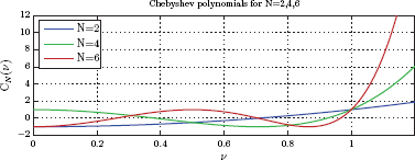
Software resources:
matex_10_2a.m
matex_10_2b.m
MATLAB Exercise 10.3: Chebyshev type-I analog filter design
In Example 10.3 a Chebyshev type-I lowpass filter with N = 3 and ε = 0.4 was designed. In this exercise we will verify the results using function cheby1(..). The second argument for the function cheby1(..) is the decibel passband tolerance Rp which is computed as
The desired filter can be obtained with the following statements:
>> N = 3;
>> omg1 = 1;
>> epsilon = 0.4;
>> Rp = 10* log10 (1+ epsilon ^2);
>> [num, den] = cheby1 (N, Rp, omg1, ’s’)
num =
0 0 0 0.6250
den =
1.0000 1.1542 1.4161 0.6250
Again the third argument ’s’ is needed for specifying that an analog filter is desired since the function cheby1(..) can be used for designing both analog and discrete-time Chebyshev type-I filters. The vectors “num” and “den” returned by the function indicate an s-domain system function
for the designed filter. Magnitude and phase characteristics of the designed filter may be graphed with the following statements:
>> omg = [-4:0.01:4];
>> H = freqs (num, den, omg);
>> plot (omg, abs (H));
>> plot (omg, angle (H));
Software resources:
matex_10_3a.m
matex_10_3b.m
MATLAB Exercise 10.4: Determining Chebyshev analog filter parameters
Design a Chebyshev type-I lowpass filter with the set of specifications
Solution: The design can be carried out using MATLAB functions cheb1ord(..) and cheby1(..) as follows:
>> omg1 = 3;
>> omg2 = 4;
>> Rp = 1;
>> As = 30;
>> N = cheb1ord (omg1, omg2, Rp, As, ’s’)
N =
7
[num , den] = cheby1 (N, Rp, omg1, ’s’)
num =
0 0 0 0 0 0 0 67.156
den =
1.000 2.769 19.585 38.577 109.961 133.315 155.766 67.156
The results correspond to a seventh-order system function
Magnitude characteristics of the designed filter may be graphed with the following statements:
>> omg = [-10:0.01:10];
>> H = freqs (num, den, omg);
>> plot (omg, abs (H)); grid ;
>> axis ([-10, 10, -0.1, 1.1]);
>> title (’|H (omega)|’);
>> xlabel (’omega (rad/s)’);
>> ylabel (’Magnitude’);
The graph produced is shown in Fig. 10.45.

Software resources:
matex_10_4a.m
matex_10_4b.m
MATLAB Exercise 10.5: Chebyshev type-II analog filter design
Design a Chebyshev type-II lowpass filter with the set of specifications
Solution: The design can be carried out using MATLAB functions cheb2ord(..) and cheby2(..) as follows:
>> omg1 = 3;
>> omg2 = 4;
>> Rp = 1;
>> As = 30;
>> N = cheb2ord (omg1, omg2, Rp, As, ’s’);
>> [num, den] = cheby2 (N, As, omg2, ’s’);
The results correspond to a seventh-order system function
Magnitude characteristics of the designed filter may be graphed with the following statements:
>> omg = [-10:0.01:10];
>> H = freqs (num, den, omg);
>> plot (omg, abs (H)); grid ;
>> axis ([-10, 10, -0.1, 1.1]);
>> title (’|H(omega)|’);
>> xlabel (’omega (rad/s)’);
>> ylabel (’Magnitude’);
The graph produced is shown in Fig. 10.46.

Software resources:
matex_10_5a.m
matex_10_5b.m
MATLAB Exercise 10.6: Lowpass to highpass filter transformation
Recall that a Chebyshev type-I analog lowpass filter was designed in MATLAB Exercise 10.3. Using it as the starting point, obtain a highpass filter with a passband edge at ωH2 = 3 rad/s.
Solution: The function lp2hp(..) can be used for this purpose. The filter of MATLAB Exercise 10.3 is redesigned and then converted to a highpass filter with the following set of statements:
>> Rp = 10* log10 (1+0.4^2);
>> [num, den] = cheby1 (3, Rp ,1, ’s’);
>> [numh, denh] = lp2hp (num, den, 3)
numh =
1.0000 -0.0000 -0.0000 0.0000
denh =
1.0000 6.7971 16.6201 43.2000
Magnitude and phase characteristics of the highpass filter may be graphed with the following statements:
>> omg = [-7:0.01:7];
>> H = freqs (numh, denh, omg);
>> plot (omg, abs (H)); grid ;
>> plot (omg, angle (H)); grid;
Software resources:
matex_10_6a.m
matex_10_6b.m
MATLAB Exercise 10.7: Lowpass to bandpass and lowpass to band-reject transformations
Using the Chebyshev filter designed in MATLAB Exercise 10.3 as a basis, design the following two filters:
A bandpass filter with the critical frequencies
A band-reject filter with the critical frequencies
Solution:
The statements listed below repeat the lowpass filter design of MATLAB Exercise 10.3 and then convert it to a bandpass filter through the use of the function lp2bp(..). The magnitude response of the resulting bandpass filter is graphed.
>> omgL1 = 1;>> epsilon = 0.4;>> Rp = 10 * log10 (1+ epsilon ^2);>> [num, den] = cheby1 (3, Rp, omgL1, ’s’);>> omgB2 = 1.5;>> omgB3 = 2.5;>> omg0 = sqrt (omgB2 * omgB3);>> B = (omgB3 - omgB2)/ omgL1 ;>> [numb, denb] = lp2bp (num, den, omg0, B)numb =0.6250 0.0000 -0.0000 -0.0000denb =1.0000 1.1542 12.6661 9.2813 47.4977 16.2305 52.7344>> omg = [-10:0.01:10];>> H = freqs (numb, denb, omg);>> plot (omg, abs (H)); grid;>> title (’|H(omega)|’);>> xlabel (’omega (rad/s)’);>> ylabel (’Magnitude’);- The statements listed below repeat the lowpass filter design of MATLAB Exercise 10.3 and then convert it to a band-reject filter through the use of the function lp2bs(..) and graph the magnitude response of the resulting band-reject filter.
>> omgL1 = 1;
>> epsilon = 0.4;>> Rp = 10 * log10 (1+ epsilon ^2);>> [num, den] = cheby1 (3, Rp, omgL1, ’s’);>> omgS1 = 1;>> omgS4 = 3.5;>> omg0 = sqrt (omgS1 * omgS4);>> B = (omgS4 - omgS1) * omgL1 ;>> [nums, dens] = lp2bs (num, den, omg0, B)nums =1.0000 -0.0000 10.5000 -0.0000 36.7500 -0.0000 42.8750dens =1.0000 16.9927 114.3754 793.9487 400.3140 208.1602 42.8750>> omg = [-10:0.01:10];>> H = freqs (nums, dens, omg);>> plot (omg, abs (H)); grid;>> title (’|H (omega)|’);>> xlabel (’omega (rad/s)’);>> ylabel (’Magnitude’);
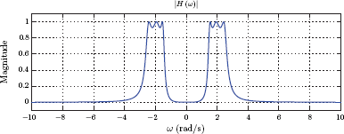
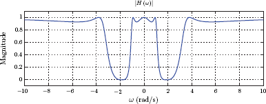
Software resources:
matex_10_7a.m
matex_10_7b.m
MATLAB Exercise 10.8: Impulse-invariant design
In Example 10.5 impulse invariance technique was used for obtaining a discrete-time filter from a Chebyshev type-I analog prototype with system function
MATLAB function impinvar(..) can be used to accomplish this task as follows:
>> T = 0.2;
>> num = [0.6250];
>> den = [1 ,1.1542 ,1.4161 ,0.6250];
>> [numz, denz] = impinvar (num, den, 1/T)
numz =
-0.0000 0.0023 0.0021
denz =
1.0000 -2.7412 2.5395 -0.7939
The results obtained correspond to the z-domain system function
which matches the answer found in Example 10.5. The magnitude and the phase of the system function may be graphed with the following statements:
>> Omg = [0:0.01:1] * pi ;
>> H = freqz (numz, denz, Omg);
>> plot (Omg, abs (H));
>> plot (Omg, angle (H));
Software resources:
matex_10_8a.m
matex_10_8b.m
MATLAB Exercise 10.9: IIR filter design using bilinear transformation
Consider again the IIR lowpass filter design problem solved in Example 10.8. In this exercise we will rely on MATLAB to solve it. Recall that the specifications for the filter to be designed were given as follows:
Even though the design problem can be solved quickly with two function calls (see MATLAB Exercise 10.10 for this alternative approach), we will opt to solve it using the three steps in Section 10.5.1. This will allow checking the intermediate results obtained in Example 10.8. The first step is to find the specifications for the analog prototype filter. Critical frequencies ω1 and ω2 for the analog prototype are found using the prewarping formula. Afterwards N and ωc are determined using the function buttord(..).
>> T = 1;
>> Rp = 2;
>> As = 20;
>> omg1 = 2/T * tan (0.2 * pi/2);
>> omg2 = 2/T * tan (0.36 * pi/2);
>> [N, omgc] = buttord (omg1, omg2, Rp, As, ’s’)
N =
4
omgc =
0.7146
The last argument of the function buttord(..) signifies that we seek the order and cutoff frequency for an analog Butterworth filter. Having determined N and ωc, the analog prototype filter can be designed using the function butter(..).
>> [num, den] = butter (N, omgc, ’s’)
num =
0 0 0 0 0.2608
den =
1.0000 1.8675 1.7437 0.9537 0.2608
Again the last argument specifies that we are designing an analog filter. The vectors “num” and “den” correspond to the analog prototype system function
If desired, magnitude and phase characteristics of the analog prototype filter may be graphed with the following lines:
>> omg = [0:0.01:5];
>> G = freqs (num, den, omg);
>> plot (omg, abs (G)); grid;
>> plot (omg, angle (G)); grid;
In step 3 the analog prototype filter is converted to a discrete-time filter using bilinear transformation. MATLAB function bilinear(..) may be used for this purpose.
>> [numz, denz] = bilinear (num, den, 1/T)
numz =
0.0065 0.0260 0.0390 0.0260 0.0065
denz =
1.0000 -2.2209 2.0861 -0.9204 0.1594
The system function for the discrete-time system is
If desired, magnitude and phase characteristics of the discrete-time filter may be graphed with the following lines:
>> Omg = [0:0.01:1] * pi;
>> H = freqz (numz, denz, Omg);
>> plot (Omg, abs (H));
>> plot (Omg, angle (H));
Software resources:
matex_10_9.m
MATLAB Exercise 10.10: IIR filter design using bilinear transformation revisited
The Butterworth IIR filter of MATLAB Exercise 10.9 can be designed quickly by using the discrete-time filter design capabilities of the functions buttord(..) and butter(..) as follows:
>> T = 1;
>> Omg1 = 0.2 * pi;
>> Omg2 = 0.36 * pi;
>> Rp = 2;
>> As = 20;
>> [N, Omgc] = buttord (Omg1/pi, Omg2/pi, Rp, As);
>> [numz, denz] = butter (N, Omgc)
numz =
0.0065 0.0260 0.0390 0.0260 0.0065
denz =
1.0000 -2.2209 2.0861 -0.9204 0.1594
Note that we leave out the last argument ’s’ to obtain discrete-time solutions directly. The result obtained is identical to that of MATLAB Exercise 10.9.
Software resources:
matex_10_10.m
MATLAB Exercise 10.11: A complete IIR filter design example
A Chebyshev type-I IIR bandpass filter is to be designed with the following set of specifications:
The specification diagram is shown in Fig. 10.49.
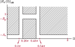
Solution: The normalized edge frequencies are
Our first step will be to use the function cheb1ord(..) to determine the minimum filter order that allows the requirements to be satisfied. In this case the cheb1ord(..) will be used without the ’s’ parameter (see MATLAB Exercise 10.4) since we want to compute the filter order from IIR digital filter specifications and not from those of the analog prototype. The following code computes N:
>> Rp = 1;
>> As = 25;
>> F1 = 0.1;
>> F2 = 0.13;
>> F3 = 0.24;
>> F4 = 0.27;
>> N = cheb1ord ([2 * F2, 2 * F3], [2 * F1, 2 * F4], Rp, As)
N =
5
The result indicates that the analog prototype is of the fifth order. Consequently, the bandpass IIR filter will be of order 10.
It is important to pay attention to the way the function cheb1ord(..) is used. The first vector in the argument list contains the two passband edge frequencies normalized in MATLAB sense, and the second vector in the argument list contains the two stopband edge frequencies also normalized in MATLAB sense. Unfortunately MATLAB defines normalized frequencies differently from the common practice. In our conventions the angular frequency Ω = π radians corresponds to the normalized frequency F = 0.5. In MATLAB conventions it corresponds to . Therefore, in specifying a discrete-time filter to MATLAB through normalized frequencies we always use twice the conventional normalized frequency values.
Once N is found, the filter is designed using the cheby1(..). Its magnitude spectrum is computed using the function freqz(..).
>> [numz , denz] = cheby1 (N, Rp, [2 * F2, 2 * F3]);
>> Omg = [-1:0.001:1] * pi;
>> H = freqz (numz ,denz , Omg);
>> plot (Omg, abs (H)); grid;
>> axis ([-pi, pi, -0.1, 1.1]);
>> title (’|H(Omega)|’);
>> xlabel (’Omega (rad)’);
>> ylabel (’Magnitude’);
The magnitude response of the filter obtained is shown in Fig. 10.50.
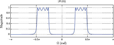
Software resources:
matex_10_11a.m
matex_10_11b.m
MATLAB Exercise 10.12: FIR filter design using Fourier series method
Using the Fourier series design method with a triangular (Bartlett) window, design a 24th-order FIR bandpass filter with passband edge frequencies Ω1 = 0.4π and Ω2 = 0.7π as shown in Fig. 10.51.
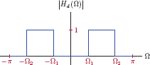
Solution: The order of the FIR filter is N − 1 = 24. Normalized passband edge frequencies are
The following two statements create a length-25 Bartlett window and then use it for designing the bandpass filter required.
>> wn = bartlett (25);
>> hn = fir1 (24, [0.4, 0.7], wn)
Some important details need to be highlighted. The function bartlett(..) uses the filter length N (this applies to other window generation functions such as hamming(..), hann(..), and blackman(..) as well). On the other hand, the design function fir1(..) uses the filter order which is N − 1. The second argument to the function fir1(..) is a vector of two normalized edge frequencies which results in a bandpass filter being designed. (A lowpass filter results if only one edge frequency is used.) The frequencies are normalized in MATLAB sense which means they must be twice our normalized frequencies.
The magnitude spectrum may be computed and graphed for the bandpass filter with impulse response in vector “hn” using the following statements.
>> Omg = [-256:255]/256 * pi;
>> H = fftshift (fft (hn ,512));
>> Omgd = [-1, -0.7, -0.7, -0.4, -0.4, 0.4, 0.4, 0.7, 0.7, 1] * pi;
>> Hd = [0, 0, 1, 1, 0, 0, 1, 1, 0, 0];
>> plot (Omg, abs (H), Omgd, Hd); grid ;
>> axis ([-pi, pi, -0.1, 1.1]);
>> title (’|H (Omega)|’);
>> xlabel (’Omega (rad)’);
>> ylabel (’Magnitude’);
The magnitude response is shown in Fig. 10.52.
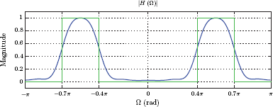
matex_10_12a.m
matex_10_12b.m
MATLAB Exercise 10.13: FIR filter design using Parks-McClellan technique
In this exercise we will explore the use of MATLAB for designing FIR filters with the Parks-McClellan algorithm. The algorithm works better if the design specifications allow for transition bands between passbands and stopbands. Consider the desired magnitude response shown in Fig. 10.53 for a bandpass filter. Only the right side of the spectrum is shown for the angular frequency range 0 ≤ Ω ≤ π.
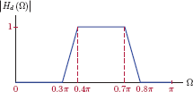
In using MATLAB function firpm(..) for Parks-McClellan FIR filter design we need to specify two vectors. The first vector lists the corner frequencies of the desired magnitude behavior shown in Fig. 10.53, normalized in MATLAB sense, and in ascending order. The first normalized frequency must be 0, and the last normalized frequency must be 1. The second vector lists the magnitude values at the corner frequencies listed in the first vector. The statements listed below create the two vectors which will be named ’frq” and “mag”.
>> frq = [0, 0.3, 0.4, 0.7, 0.8, 1];
>> mag = [0, 0, 1, 1, 0, 0];
An easy method of checking the correctness of the two vectors ’frq” and “mag” is to use them as arguments to the function plot(..) as
>> plot (pi * frq, mag);
The graph produced should be identical to the desired magnitude behavior in Fig. 10.53. The FIR bandpass filter is designed, and its magnitude spectrum is graphed through the following statements:
>> hn = firpm (24, frq, mag)
>> Omg = [0:255]/256 * pi;
>> H = fft (hn, 512);
>> H = H (1:256);
>> plot (Omg, abs (H),pi * frq, mag);
>> axis ([0, pi, -0.1, 1.1]);
>> title (’|H(Omega)|’);
>> xlabel (’Omega (rad)’);
>> ylabel (’Magnitude’);
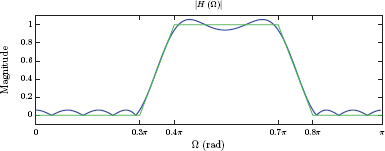
It is also possible to use weight factors in the design. The following statement leads to a design that emphasizes better accuracy in the passband in exchange for some degradation in stopband performance.
>> hn = firpm (24, frq, mag, [1, 10, 1])
Finally, increasing the filter order improves the performance further. A 44th-order FIR filter is obtained by
>> hn = firpm (44, frq, mag, [1, 10, 1])
Magnitude characteristics of the last two designs are shown in Fig. 10.55.

Magnitude response of 24th-order FIR filter with uneven weights, (b) magnitude response of 44th-order FIR filter.
Software resources:
matex_10_13a.m
matex_10_13b.m
matex_10_13c.m
Problems
- 10.1. Consider the RC circuit used in Example 10.1 and shown in Fig. 10.4. Let the parameter values be R = 1 kΩ and C = 1 μF.
- Find the frequency range in Hertz in which the magnitude of the system function exhibits 1 percent or less deviation from its value at ω = 0.
- For the frequency range found in part (a) determine how much the phase characteristic deviates from a straight line. Determine the endpoints of the phase characteristic in the range of interest, and compare them to the endpoints of a straight line with the appropriate slope.
- Find the variation in the time delay over the frequency range established in part (a).
- Repeat parts (a) through (c) if 2 percent variation in magnitude is allowed.
- 10.2. Consider a second-order lowpass filter with the system function
- Find the frequency range in Hz in which the magnitude of the system function exhibits 1 percent or less deviation from its value at ω = 0.
- For the frequency range found in part (a) determine how much the phase characteristic deviates from a straight line. Determine the endpoints of the phase characteristic in the range of interest, and compare to the endpoints of a straight line with the appropriate slope.
- Find the variation in the time delay over the frequency range established in part (a).
- Repeat parts (a) through (c) if 2 percent variation in magnitude is allowed.
- 10.3. The magnitude spectrum of an ideal lowpass filter is shown in Fig. P.10.3. The time delay is to be td = 0.1 s for all frequencies.
- Write a mathematical expression for the system function HLP (f).
- Determine the impulse response hLP (t).
- Sketch the impulse response found in part (b).
- 10.4. The magnitude spectrum of an ideal bandpass filter is shown in Fig. P.10.4. The time delay is to be td = 0.3 s for all frequencies.
- Write a mathematical expression for the system function HBP (f).
- Determine the impulse response hBP (t).
- Sketch the impulse response found in part (b).
- 10.5. Design a fourth-order Butterworth analog lowpass filter with 3-dB cutoff frequency of ωc = 2 rad/s. Find its poles and construct the system function H (s).
- 10.6. A Butterworth analog lowpass filter is to be designed with the following specifications:
Using the method presented in Section 10.4.1 determine the filter order N and the 3-dB cutoff frequency ωc. Do not actually design the filter.
- 10.7. Consider the problem of determining Butterworth analog lowpass filter parameters from design specifications. First N is determined from Eqn. (10.65). In general it is not an integer, and must be rounded up to the nearest integer. This rounding up causes the tolerance specifications to be exceeded in the designed filter.
- If Eqn. (10.62) is used for computing ωc, then specifications are met exactly at the passband edge ω = ω1 and exceeded at the stopband edge ω = ω2.
- If Eqn. (10.63) is used for computing ωc, then specifications are met exactly at the stopband edge ω = ω2 and exceeded at the passband edge ω = ω1.
An alternative would be to divide the excess tolerance equally (in a dB sense) between the passband and the stopband. Derive the general solution for ωc to accomplish this.
- 10.8. Design a fourth-order Chebyshev type-I analog filter with a passband edge frequency of ω1 = 2 rad/s and ε = 0.3. Find the poles of the filter and then construct the system function H (s).
- 10.9. Design a fourth-order Chebyshev type-II analog filter with a stopband edge frequency of ω2 = 2 rad/s and ε = 0.3. Find the poles of the filter and then construct the system function H (s).
- 10.10. An analog lowpass filter is needed with the following specifications:
- Determine N and ωc for a Butterworth filter that meets the requirements. Find the system function for the corresponding filter.
- Determine N and ε for a Chebyshev type-I filter that meets the requirements. Find the system function for the corresponding filter.
- Determine N and ε for a Chebyshev type-II filter that meets the requirements. Find the system function for the corresponding filter.
- 10.11. Consider the lowpass to bandpass filter transformation given by Eqn. (10.124). Show that the parameters ε0 and B must be chosen as given by Eqn. (10.127) in order to satisfy the conditions given by Eqns. (10.125) and (10.126).
Hint: Let s = jω and λ = jp. Write the relationship between the radian frequencies ω and p and sketch ω as a function of p. Impose the conditions of Eqns. (10.125) and (10.126) and solve for the unknown parameters.
- 10.12. Consider the lowpass to band-reject filter transformation given by Eqn. (10.128). Show that the parameters ω0 and B must be chosen as given by Eqn. (10.131) in order to satisfy the conditions given by Eqns. (10.129) and (10.130).
Hint: Let s = jω and λ = jp. Write the relationship between the radian frequencies ω and p and sketch ω as a function of p. Impose the conditions of Eqns. (10.129) and (10.130) and solve for the unknown parameters.
- 10.13. Consider a lowpass filter with the system function
This filter is to be converted to a highpass filter with system function H (λ) by means of the transformation s = ω0/λ.
- Determine ω0 so that the frequency 2 rad/s for the lowpass filter corresponds to the frequency 5 rad/s for the highpass filter.
- Using the value of ω0 found in part (a), determine the frequency for the highpass filter that corresponds to the frequency 6 rad/s for the lowpass filter.
- Determine the system function H (λ) for the highpass filter. Evaluate its magnitude at the frequency ω = 5 rad/s and verify that it is equal to the magnitude of the lowpass filter at ω = 2 rad/s.
- 10.14. A Butterworth analog highpass filter is to be designed with the following specifications:
- Find the corresponding specifications ωL1, ωL2, Rp and As for an appropriate lowpass prototype filter.
- Determine the parameters N and ωc for the lowpass prototype filter.
- Design the lowpass prototype filter. Find its poles, and construct its system function G (s).
- Convert the lowpass prototype filter to a highpass filter using the appropriate transformation. Determine the system function H (λ).
- Evaluate the decibel magnitude of the highpass filter at the frequencies ωH1 and ωH2. Verify that the designed filter meets the requirements.
- 10.15. An analog filter with the system function
is to be used as a prototype for the design of a discrete-time filter through the impulse invariance technique.
- Find the impulse response g (t) of the analog prototype filter.
Obtain the impulse response of the discrete-time filter as a sampled and scaled version of the analog prototype impulse response, that is,
Use the sampling interval T = 0.5 s.
- Determine the system function H (z) of the discrete-time filter.
- 10.16. An analog filter with the system function
is to be used as a prototype for the design of a discrete-time filter through bilinear transformation. Using T = 0.5 s, convert the analog prototype system function G (s) to a discrete-time filter system function H (z).
- 10.17. The impulse response of an FIR filter is
where N, the length of the FIR filter, is even.
Show that, if
then the system function H (Ω) is in the form
where A (Ω) is some function that is purely real.
Show that, if
then the system function H (Ω) is in the form
where B (Ω) is some function that is purely real.
- 10.18. Repeat the proofs in Problem 10.17 for the case where N is odd.
- 10.19. Using the Fourier series design method with a Hamming window, design a length-19 FIR filter to approximate the ideal bandpass magnitude characteristic shown in Fig. P.10.19.
- 10.20. In the use of Fourier series design method for FIR filters we have focused on designing filters with an odd number of coefficients. This was necessitated by step 2 of the design process where the ideal impulse response hd[n] is truncated to the interval −M ≤ n ≤ M resulting in filter length N =2M + 1, always an odd value.
It is possible to modify the method slightly to allow the design of both odd-length and even-length filters. The key is to anticipate the correct time delay due to the linear phase characteristics of the final design, and make it part of the specifications. Let the ideal spectrum to be approximated be given by
Show that, by computing the ideal impulse response as the inverse DTFT of Hd (Ω) and truncating the result to retain samples in the interval n = 0,...,N − 1, a linear-phase FIR filter can be obtained for both odd and even values of N.
- 10.21. Refer to Problem 10.20. If a window function is to be used with the modified design technique described in Problem 10.20, its sample amplitudes need to be specified for the index range n = 0,...,N − 1. In addition, window samples must have the symmetry property
Modify the window function definitions given in Eqns. (10.180) through (10.183) to fit this form.
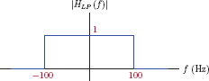
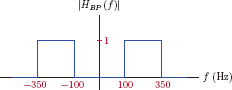

MATLAB Problems
- 10.22. Consider again the RC circuit of Problem 10.1. Develop a MATLAB script to graph magnitude, phase and time delay characteristics of the circuit in a specified range of frequency −f0 < f < f0.
- Using the script developed, graph the characteristics for the frequency range found in part (a) of Problem 10.1.
- Repeat for for the frequency range found in part (d) of Problem 10.1.
- 10.23. Consider the second-order lowpass filter of Problem 10.2. Develop a MATLAB script to graph magnitude, phase and time delay characteristics of the system in a specified range of frequency −f0 < f < f0.
- Using the script developed, graph the characteristics for the frequency range found in part (a) of Problem 10.2.
- Repeat for for the frequency range found in part (d) of Problem 10.2.
- 10.24.
- Develop a MATLAB function ss_ilp(..) to compute the impulse response of an ideal lowpass filter with the system function
The syntax of your function should be
h = ss_ilp (omg0 ,td ,t)where “omg0” and “td” are parameters of the ideal lowpass filter, and “t” is the vector of time instants at which the impulse response if to be evaluated.
- Write a script to test the function ss_ilp(..) for several sets of parameter values.
- Develop a MATLAB function ss_ilp(..) to compute the impulse response of an ideal lowpass filter with the system function
- 10.25.
Develop a MATLAB function ss_ibp(..) to compute the impulse response of an ideal bandpass filter with the system function
The syntax of your function should be
h = ss_ibp (omg1 ,omg2 ,td ,t)where “omg1”, “omg2” and “td” are parameters of the ideal lowpass filter, and “t” is the vector of time instants at which the impulse response if to be evaluated. The function ss_ibp(..) should internally utilize the function ss_ilp(..) developed in Problem 10.24.
- Write a script to test the function ss_ibp(..) for several sets of parameter values.
- 10.26. Refer to the Butterworth analog lowpass filter design considered in Problem 10.5. Design the same filter using MATLAB. Graph the magnitude and the phase characteristics of the designed filter.
- 10.27. Refer to Problem 10.6. Using the values of N and ωc found in Problem 10.6 and the MATLAB function butter(..) design the filter. Compute and graph the dB magnitude response of the filter and verify that it satisfies the design specifications.
- 10.28.
- Design the filter specified in Problem 10.8 using MATLAB.
- Compute and graph the decibel magnitude response and verify that it meets the requirements of the design.
- Graph the pole-zero diagram of the system function.
- 10.29.
- Design the filter specified in Problem 10.9 using MATLAB.
- Compute and graph the decibel magnitude response and verify that it meets the requirements of the design.
- Graph the pole-zero diagram of the system function.
- 10.30. Refer to Problem 10.10.
- Repeat each design (Butterworth, Chebyshev type-I and Chebyshev type-II) using appropriate MATLAB functions. Compare to the results of hand calculations obtained in Problem 10.10.
- Compute and graph the magnitude response of each design.
- Compute and graph the decibel magnitude responses of all three designs on the same coordinate system.
- 10.31. Repeat the Butterworth analog highpass design in Problem 10.14 using MATLAB functions buttord(..), butter(..) and lp2hp(..). Afterwards compute and graph the decibel magnitude of the highpass filter and check the decibel tolerance values at the two critical frequencies.
- 10.32. Refer to the discrete-time filter designed in Problem 10.15 using the impulse invariance method with the sampling interval T = 0.5 s.
- Using the function impinvar(..) repeat the design process of Problem 10.15. Compare the result obtained for H (z) to the one found in Problem 10.15.
- Using MATLAB, compute and graph the magnitude response of the analog prototype filter in the frequency interval −π/T ≤ ω ≤ π/T.
- Compute and graph the magnitude response of the discrete-time filter in the angular frequency interval −π ≤ Ω ≤ π.
Suppose that the discrete-time filter is used for processing a continuous-time signal as shown in Fig. P.10.32.
Determine the relationship between the frequencies ω and Ω. Based on that relationship, compute and graph the overall magnitude response of the system in Fig. P.10.32 simultaneously with the magnitude response of the analog prototype filter for comparison. In other words, compute and graph |Ya (ω)/Xa (ω)| and |G (ω)|.
- 10.33. Repeat Problem 10.32 using a sampling interval of T = 0.25 s instead of T = 0.5 s. Comment on how this change affects the overall performance of the analog system in Fig. P.10.32 that utilizes a discrete-time filter.
- 10.34. Refer to the discrete-time filter designed in Problem 10.16 using the bilinear transformation method with the sampling interval T = 0.5 s.
- Using the function bilinear(..) repeat the design process of Problem 10.16. Compare the result obtained for H (z) to the one found in Problem 10.16.
- Using MATLAB, compute and graph the magnitude response of the analog prototype filter in the frequency interval −π/T ≤ ω ≤ π/T.
- Compute and graph the magnitude response of the discrete-time filter in the angular frequency interval −π ≤ Ω ≤ π.
- Suppose that the discrete-time filter is used for processing a continuous-time signal as shown in Fig. P.10.32. Compute and graph the overall magnitude response of the system in Fig. P.10.32 simultaneously with the magnitude response of the analog prototype filter for comparison. In other words, compute and graph |Ya (ω)/Xa (ω)| and |G (ω)|.
- 10.35. Refer to the FIR filter specified in Problem 10.19.
- Write a script to compute and graph the magnitude response of the length-15 filter designed manually in Problem 10.19.
- Write a script to design a length-45 filter to meet the same specifications. Compute and graph the decibel magnitude characteristics of the length-15 and length-45 designs in a superimposed fashion for comparison.
- Repeat the length-45 design using a Blackman window instead of a Hamming window. Compute and graph the decibel magnitude characteristics of the two length-45 designs together and compare.
- 10.36.
Develop a MATLAB function ss_fir1(..) to design a FIR lowpass filter of any order N using the technique explored in Problem 10.20. The syntax of the function should be
hd = ss_fir1 (Omgc ,N)where “Omgc” is the cutoff frequency in radians, and “N” is the filter length. The returned vector “hd” holds samples of the impulse response. No windowing is done within this function; a window function may be applied to the vector “hd” separately if desired.
- Test the function developed in part (a) by using it to design a length-36 lowpass FIR filter with angular cutoff frequency Ωc = 0.4π radians. Compute and graph the magnitude response of the designed filter.
MATLAB Projects
- 10.37. FIR filters obtained through the use of the Fourier series design method suffer from Gibbs oscillations especially around the discontinuities of the desired magnitude behavior. We have seen that using a window function in the design process alleviates this problem. Another solution is to change the desired filter spectrum to a more realistic one. Consider the desired lowpass filter magnitude spectrum shown in Fig. P.10.37(a). Two frequencies Ω1 and Ω2 define the edges of the passband and the stopband. Between the two frequencies is a transition band. If this magnitude characteristic is sampled at the DFT frequencies we obtain
as shown in Fig. P.10.37(b).
With the addition of a linear phase term, H[k] is found as
where M is the delay of the filter computed as M = (N − 1)/2. The impulse response of the FIR filter is found as the inverse DFT of H [k]:
This is the basis of the design method known as frequency-sampling design.
- Using the idea outlined, develop a MATLAB function ss_fir2(..) with the following syntax:
h = ss_fir2 (Omg ,mag ,N)The vector “Omg” holds the corner frequencies of the desired magnitude spectrum starting with 0 and ending with 2π. For example, for a lowpass filter with edge frequencies Ω1 = 0.3π and Ω2 = 0.5π the vector “Omg” would have the elements
The vector “mag” holds desired magnitude values at the corner frequencies in the vector “Omg”. For the example above, the vector “mag” would have the elements
As a simple test, the statement
>> plot (Omg, mag)should graph the desired magnitude in the interval 0 ≤ Ω ≤ 2π.
- Use the function ss_fir2(..) to design a length-35 lowpass FIR linear-phase filter with the critical frequencies Ω1 = 0.2π and Ω2 = 0.3π. Compute and graph the magnitude response of the designed filter.
- Using the idea outlined, develop a MATLAB function ss_fir2(..) with the following syntax:
- 10.38. Refer to the function ss_iir2(..) developed in MATLAB Exercise 8.12 in Chapter 8 for implementing a second-order section with system function
One of the input arguments of the function ss_iir2(..) is a vector of filter coefficients in a prescribed order:
GUI-based MATLAB program fdatool has the capability to export the coefficients of a designed filter to the workspace as a “SOS matrix” which corresponds to an implementation of the filter in the form of second-order cascade sections. Each row of the “SOS matrix” contains the coefficients of one second-order section in the same order given above.
- Develop a MATLAB function ss_iirsos(..) for implementing an IIR filter designed using the program fdatool(..). Its syntax should be
out = ss_iirsos (inp ,sos, gains)The matrix “sos” is the coefficient matrix exported from fdatool(..) using the menu selections file, export. The vector “gains” is the vector of gain factors for each second-order section. It is also exported from fdatool(..). The vector “inp” holds samples of the input signal. The computed output signal is returned in vector “out”. The function ss_iirsos(..) should internally utilize the function ss_iir2(..) for implementing the filter in cascade.
- Use fdatool(..) to design an elliptic bandpass filter with passband edges at Ω2 = 0.4π, Ω3 = 0.7π and stopband edges at Ω1 = 0.3π, Ω4 = 0.8π. The passband ripple must not exceed 1 dB, and the stopband attenuation must be at least 30 dB. Export the coefficients and gain factors of the designed filter to MATLAB workspace.
- Use the function ss_iirsos(..) to compute the unit-step response of the designed filter. Compare to the step response computed by the program fdatool(..).
- Develop a MATLAB function ss_iirsos(..) for implementing an IIR filter designed using the program fdatool(..). Its syntax should be
