
Fourier Analysis for Discrete-Time Signals and Systems
Chapter Objectives
- Learn the use of discrete-time Fourier series for representing periodic signals using orthogonal basis functions.
- Learn the discrete-time Fourier transform (DTFT) for non-periodic signals as an extension of discrete-time Fourier series for periodic signals.
- Study properties of the DTFT. Understand energy and power spectral density concepts.
- Explore frequency-domain characteristics of DTLTI systems. Understand the system function concept.
- Learn the use of frequency-domain analysis methods for solving signal-system interaction problems with periodic and non-periodic input signals.
- Understand the fundamentals of the discrete Fourier transform (DFT) and fast Fourier transform (FFT). Learn how to compute linear convolution using the DFT.
5.1 Introduction
In Chapter 1 and Chapter 3 we have developed techniques for analyzing discrete-time signals and systems from a time-domain perspective. A discrete-time signal can be modeled as a function of the sample index. A DTLTI system can be represented by means of a constant-coefficient linear difference equation, or alternatively by means of an impulse response. The output signal of a DTLTI system can be determined by solving the corresponding difference equation or by using the convolution operation.
In this chapter frequency-domain analysis methods are developed for discrete-time signals and systems. Section 5.2 focuses on analyzing periodic discrete-time signals in terms of their frequency content. Discrete-time Fourier series (DTFS) is presented as the counterpart of the exponential Fourier series (EFS) studied in Chapter 4 for continuous-time signals. Frequency-domain analysis methods for non-periodic discrete-time signals are presented in Section 5.3 through the use of the discrete-time Fourier transform (DTFT). Energy and power spectral density concepts for discrete-time signals are introduced in Section 5.4. Section 5.5, Section 5.6 and Section 5.7 cover the application of frequency-domain analysis methods to the analysis of DTLTI systems. Section 5.8 introduces the discrete Fourier transform (DFT) and the fast Fourier transform (FFT).
5.2 Analysis of Periodic Discrete-Time Signals
In Section 4.2 of Chapter 4 we have focused on expressing continuous-time periodic signals as weighted sums of sinusoidal or complex exponential basis functions. It is also possible to express a discrete-time periodic signal in a similar manner, as a linear combination of discrete-time periodic basis functions. In this section we will explore one such periodic expansion referred to as the discrete-time Fourier series (DTFS). In the process we will discover interesting similarities and differences between DTFS and its continuous-time counterpart, the exponential Fourier series (EFS) that was discussed in Section 4.2. One fundamental difference is regarding the number of series terms needed. We observed in Chapter 4 that a continuous-time periodic signal may have an infinite range of frequencies, and therefore may require an infinite number of harmonically related basis functions. In contrast, discrete-time periodic signals contain a finite range of angular frequencies, and will therefore require a finite number of harmonically related basis functions. We will see in later parts of this section that a discrete-time signal with a period of N samples will require at most N basis functions.
5.2.1 Discrete-Time Fourier Series (DTFS)
Consider a discrete-time signal periodic with a period of N samples, that is, for all n. As in Chapter 4 periodic signals will be distinguished through the use of the tilde (˜) character over the name of the signal. We would like to explore the possibility of writing as a linear combination of complex exponential basis functions in the form
using a series expansion
Two important questions need to be answered:
- How should the angular frequencies Ωk be chosen?
- How many basis functions are needed? In other words, what should be the limits of the summation index k in Eqn. (5.2)?
Intuitively, since the period of is N samples long, the basis functions used in constructing the signal must also be periodic with N. Therefore we require
for all n. Substituting Eqn. (5.1) into Eqn. (5.3) leads to
For Eqn. (5.4) to be satisfied we need ejΩkN = 1, and consequently ΩkN = 2πk. The angular frequency of the basis function φk[n] must be
leading to the set of basis functions
Using φk[n] found, the series expansion of the signal is in the form
To address the second question, it can easily be shown that only the first N basis functions φ0[n],φ1[n],...,φN−1[n] are unique; all other basis functions, i.e., the ones obtained for k < 0 or k ≥ N, are duplicates of the basis functions in this set. To see why this is the case, let us write φk+N [n]:
Factoring Eqn. (5.8) into two exponential terms and realizing that ej2πn = 1 for all integers n we obtain
Since φk+N[n] is equal to φk[n], we only need to include N terms in the summation of Eqn. (5.7).
The signal can be constructed as
As a specific example, if the period of the signal is N = 5, then the only basis functions that are unique would be
Increasing the summation index k beyond k = 4 would not create any additional unique terms since φ5[n] = φ0[n], φ6[n]= φ1[n], and so on.
Eqn. (5.10) is referred to as the discrete-time Fourier series (DTFS) expansion of the periodic signal . The coefficients used in the summation of Eqn. (5.10) are the DTFS coefficients of the signal .
Example 5.1: DTFS for a discrete-time sinusoidal signal
Determine the DTFS representation of the signal .
Solution: The angular frequency of the signal is
and it corresponds to the normalized frequency
Since normalized frequency F0 is an irrational number, the signal specified is not periodic (refer to the discussion in Section 1.4.4 of Chapter 1). Therefore it cannot be represented in series form using periodic basis functions. It can still be analyzed in the frequency domain, however, using the discrete-time Fourier transform (DTFT) which will be explored in Section 5.3.
Example 5.2: DTFS for a discrete-time sinusoidal signal revisited
Determine the DTFS representation of the signal .
Solution: The angular frequency of the signal is
and the corresponding normalized frequency is
Based on the normalized frequency, the signal is periodic with a period of N = 1/F0 = 10 samples. A general formula for obtaining the DTFS coefficients will be derived later in this section. For the purpose of this example, however, we will take a shortcut afforded by the sinusoidal nature of the signal , and express it using Euler’s formula:
The two complex exponential terms in Eqn. (5.11) correspond to φ1[n] and φ−1[n], therefore their coefficients must be and , respectively. As a result we have
As discussed in the previous section we would like to see the series coefficients in the index range k = 0,...,N − 1 where N is the period. In this case we need to obtain for k = 0,..., 9. The basis functions have the property
The term φ−1[n] in Eqn. (5.11) can be written as
DTFS coefficients are
The signal and its DTFS spectrum are shown in Fig. 5.1.
![Figure showing (a) The signal x˜[n] for Example 5.2, and (b) its DTFS spectrum.](http://imgdetail.ebookreading.net/data/1/9781466598546/9781466598546__signals-and-systems__9781466598546__image__417x001.png)
Software resources:
ex_5_2.m
Example 5.3: DTFS for a multi-tone signal
Determine the DTFS coefficients for the signal
Solution: The two angular frequencies Ω1 = 0.2π and Ω2 = 0.3π radians correspond to normalized frequencies F1 = 0.1 and F2 = 0.15 respectively. The normalized fundamental frequency of is F0 = 0.05, and it corresponds to a period of N = 20 samples. Using this value of N, the angular frequencies of the two sinusoidal terms of are
and
We will use Euler’s formula to write in the form
We know from the periodicity of the DTFS representation that
The signal and its DTFS spectrum are shown in Fig. 5.2.
![Figure showing (a) The signal x˜[n] for Example 5.3, (b) magnitude of the DTFS spectrum, and (c) phase of the DTFS spectrum.](http://imgdetail.ebookreading.net/data/1/9781466598546/9781466598546__signals-and-systems__9781466598546__image__418x001.png)
(a) The signal for Example 5.3, (b) magnitude of the DTFS spectrum, and (c) phase of the DTFS spectrum.
Software resources:
ex_5_3.m
Finding DTFS coefficients
In Examples 5.2 and 5.3 the DTFS coefficients for discrete-time sinusoidal signals were easily determined since the use of Euler’s formula gave us the ability to express those signals in a form very similar to the DTFS expansion given by Eqn. (5.7). In order to determine the DTFS coefficients for a general discrete-time signal we will take advantage of the orthogonality of the basis function set {φk[n], k = 0,...,N − 1}. It can be shown that (see Appendix D)
To derive the expression for the DTFS coefficients, let us first write Eqn. (5.10) using m instead of k as the summation index:
Multiplication of both sides of Eqn. (5.7) by e−j(2π/N)kn leads to
Summing the terms on both sides of Eqn. (5.17) for n = 0,...,N − 1, rearranging the summations, and using the orthogonality property yields
The DTFS coefficients are computed from Eqn. (5.18) as
In Eqn. (5.19) the DTFS coefficients are computed for the index range k = 0,...,N − 1 since those are the only coefficient indices that are needed in the DTFS expansion in Eqn. (5.10). If we were to use Eqn. (5.19) outside the specified index range we would discover that
for all integers r. The DTFS coefficients evaluated outside the range k = 0,...,N − 1 exhibit periodic behavior with period N. This was evident in Examples 5.2 and 5.3 as well. The development so far can be summarized as follows:
Discrete-Time Fourier Series (DTFS):
Synthesis equation:
Analysis equation:
Note that the coefficients are computed for all indices k in Eqn. (5.22), however, only the ones in the range k = 0,...,N − 1 are needed in constructing the signal in Eqn. (5.21). Due to the periodic nature of the DTFS coefficients , the summation in the synthesis equation can be started at any arbitrary index, provided that the summation includes exactly N terms. In other words, Eqn. (5.21) can be written in the alternative form
Example 5.4: Finding DTFS representation
Consider the periodic signal defined as
and shown in Fig. 5.3. Determine the DTFS coefficients for . Afterwards, verify the synthesis equation in Eqn. (5.21).
![Figure showing the signal x˜[n] for Example 5.4.](http://imgdetail.ebookreading.net/data/1/9781466598546/9781466598546__signals-and-systems__9781466598546__image__420x001.png)
Solution: Using the analysis equation given by Eqn. (5.22) the DTFS coefficients are
Evaluating Eqn. (5.24) for k = 0,..., 4 we get
The signal can be constructed from DTFS coefficients as
Software resources:
ex_5_4a.m
ex_5_4b.m
Example 5.5: DTFS for discrete-time pulse train
Consider the periodic pulse train defined by
where N > 2L + 1 as shown in Fig. 5.4. Determine the DTFS coefficients of the signal in terms of L and N.
![Figure showing the signal x˜[n] for Example 5.5.](http://imgdetail.ebookreading.net/data/1/9781466598546/9781466598546__signals-and-systems__9781466598546__image__421x001.png)
Solution: Using Eqn. (5.22) the DTFS coefficients are
The closed form expression for a finite-length geometric series is (see Appendix C for derivation)
Using Eqn. (C.13) with a = e−j(2π/N)k, L1 = −L and L2 = L, the closed form expression for is
In order to get symmetric complex exponentials in Eqn. (5.25) we will multiply both the numerator and the denominator of the fraction on the right side of the equal sign with ejπk/N resulting in
which, using Euler’s formula, can be simplified to
The coefficient needs special attention. Using L’Hospital’s rule we obtain
The DTFS representation of the signal is
The DTFS coefficients are graphed in Fig. 5.5 for N = 40 and L = 3, 5, and 7.
![Figure showing the DTFS coefficients of the signal x˜[n] of Example 5.5 for N = 40 and (a) L = 3, (b) L = 5, and (c) L = 7.](http://imgdetail.ebookreading.net/data/1/9781466598546/9781466598546__signals-and-systems__9781466598546__image__422x001.png)
The DTFS coefficients of the signal of Example 5.5 for N = 40 and (a) L = 3, (b) L = 5, and (c) L = 7.
Software resources:
ex_5_5.m
Interactive Demo: dtfs_demo1
The demo program in “dtfs_demo1.m” provides a graphical user interface for computing the DTFS representation of the periodic discrete-time pulse train of Example 5.5. The period is fixed at N = 40 samples. The parameter L can be varied from 0 to 19. The signal and its DTFS coefficients are displayed.
- Set L = 0. Observe the coefficients and comment.
- Increment L to 2, 3, 4,... and observe the changes to DTFS coefficients. Pay attention to the outline (or the envelope) of the coefficients. Can you identify a pattern that emerges as L is incremented.
Software resources:
dtfs_demo1.m
Software resources: |
See MATLAB Exercises 5.1 and MATLAB Exercise 5.2. |
5.2.2 Properties of the DTFS
In this section we will summarize a few important properties of the DTFS representation of a periodic signal. To keep the notation compact, we will denote the relationship between the periodic signal and its DTFS coefficients as
Periodicity
DTFS coefficients are periodic with the same period N as the signal .
Given
it can be shown that
Periodicity of DTFS coefficients follows easily from the analysis equation given by Eqn. (5.22).
Linearity
Let and be two signals, both periodic with the same period, and with DTFS representations
It can be shown that
for any two arbitrary constants α1 and α2.
Linearity property is easily proven starting with the synthesis equation in Eqn. (5.21).
Time shifting
Given that
it can be shown that
Time shifting the signal causes the DTFS coefficients to be multiplied by a complex exponential function.
Consistency check: Let the signal be time shifted by exactly one period, that is, m = N. We know that due to the periodicity of . The exponential function on the right side of Eqn. (5.30) would be e−j(2π/N)kN = 1, and the DTFS coefficients remain unchanged, as expected.
Symmetry of DTFS coefficients
Conjugate symmetry and conjugate antisymmetry properties were defined for discrete-time signals in Section 1.4.6 of Chapter 1. Same definitions apply to DTFS coefficients as well. A conjugate symmetric set of coefficients satisfy
for all k. Similarly, the coefficients form a conjugate antisymmetric set if they satisfy
for all k. For a signal which is periodic with N samples it is customary to use the DTFS coefficients in the index range k = 0,...,N − 1. The definitions in Equation (5.31) and Equation (5.32) can be adjusted in terms of their indices using the periodicity of the DTFS coefficients. Since , a conjugate symmetric set of DTFS coefficients have the property
Similarly, a conjugate antisymmetric set of DTFS coefficients have the property
If the signal is real-valued, it can be shown that its DTFS coefficients form a conjugate symmetric set. Conversely, if the signal is purely imaginary, its DTFS coefficients form a conjugate antisymmetric set.
Symmetry of DTFS coefficients:
Polar form of DTFS coefficients
DTFS coefficients can be written in polar form as
If the set is conjugate symmetric, the relationship in Eqn. (5.33) leads to
using the polar form of the coefficients. The consequences of Eqn. (5.38) are obtained by equating the magnitudes and the phases on both sides.
Conjugate symmetric coefficients:
It was established in Eqn. (5.35) that the DTFS coefficients of a real-valued are conjugate symmetric. Based on the results in Equation (5.39) and Equation (5.40) the magnitude spectrum is an even function of k, and the phase spectrum is an odd function of k.
Similarly, if the set is conjugate antisymmetric, the relationship in Eqn. (5.34) reflects on polar form of as
The negative sign on the right side of Eqn. (5.41) needs to be incorporated into the phase since we could not write (recall that magnitude must to be non-negative). Using e∓jπ = −1, Eqn. (5.41) becomes
The consequences of Eqn. (5.42) are summarized below.
Conjugate antisymmetric coefficients:
A purely imaginary signal leads to a set of DTFS coefficients with conjugate antisymmetry. The corresponding magnitude spectrum is an even function of k as suggested by Eqn. (5.43). The phase spectrum is neither even nor odd.
Example 5.6: Symmetry of DTFS coefficients
Recall the real-valued periodic signal of Example 5.4 shown in Fig. 5.3. Its DTFS coefficients were found as
It can easily be verified that coefficients form a conjugate symmetric set. With N = 5 we have
DTFS spectra of even and odd signals
If the real-valued signal is an even function of index n, the resulting DTFS spectrum is real-valued for all k.
Conversely it can also be proven that, if the real-valued signal has odd-symmetry, the resulting DTFS spectrum is purely imaginary.
Example 5.7: DTFS symmetry for periodic waveform
Explore the symmetry properties of the periodic waveform shown in Fig. 5.6. One period of has the sample amplitudes
![Figure showing the signal x˜[n] for Example 5.7.](http://imgdetail.ebookreading.net/data/1/9781466598546/9781466598546__signals-and-systems__9781466598546__image__426x001.png)
Solution: The DTFS coefficients for are computed as
and are listed for k = 0,..., 8 in Table 5.1 along with magnitudes and phase values for each. Symmetry properties can be easily observed. The signal is real-valued, therefore the DTFS spectrum is conjugate symmetric:
DTFS coefficients for the pulse train of Example 5.7.
Furthermore, the odd symmetry of causes coefficients to be purely imaginary:
In terms of the magnitude values we have
For the phase angles the following relationships hold:
The phase values for and are insignificant since the corresponding magnitude values and are equal to zero.
Software resources:
ex_5_7.m
Periodic convolution
Consider the convolution of two discrete-time signals defined by Eqn. (3.128) and repeated here for convenience:
This summation would obviously fail to converge if both signals x[n] and h[n] happen to be periodic with periods of N. For such a case, a periodic convolution operator can be defined as
Eqn. (5.47) is essentially an adaptation of the convolution sum to periodic signals where the limits of the summation are modified to cover only one period (we are assuming that both and have the same period N). It can be shown that (see Problem 5.7) the periodic convolution of two signals and that are both periodic with N is also periodic with the same period.
Example 5.8: Periodic convolution
Two signals and , each periodic with N = 5 samples, are shown in Fig. 5.7(a) and (b). Determine the periodic convolution
![Figure showing Signals x˜[n] and h˜[n] for Example 5.4.](http://imgdetail.ebookreading.net/data/1/9781466598546/9781466598546__signals-and-systems__9781466598546__image__428x001.png)
Solution: Sample amplitudes for one period are
and
The periodic convolution is given by
To start, let n = 0. The terms and are shown in Fig. 5.8. The main period of each signal is indicated with sample amplitudes colored blue. The shaded area contains the terms included in the summation for periodic convolution. The sample is computed as
![Figure showing the terms ˜x[k] and ˜h[0 − k] in the convolution sum.](http://imgdetail.ebookreading.net/data/1/9781466598546/9781466598546__signals-and-systems__9781466598546__image__429x001.png)
Next we will set n = 1. The terms and are shown in Fig. 5.9.
![Figure showing the terms ˜x[k] and ˜h[1 − k] in the convolution sum.](http://imgdetail.ebookreading.net/data/1/9781466598546/9781466598546__signals-and-systems__9781466598546__image__429x002.png)
The sample is computed as
Finally, for n = 2 the terms involved in the summation are shown in Fig. 5.10.
![Figure showing the terms ˜x[k] and ˜h[2 − k] in the convolution sum.](http://imgdetail.ebookreading.net/data/1/9781466598546/9781466598546__signals-and-systems__9781466598546__image__429x003.png)
The sample is computed as
Continuing in this fashion, it can be shown that and . Thus, one period of the signal is
The signal is shown in Fig. 5.11.
![Figure showing Periodic convolution result ˜y[n] for Example 5.8.](http://imgdetail.ebookreading.net/data/1/9781466598546/9781466598546__signals-and-systems__9781466598546__image__430x001.png)
The periodic convolution property of the discrete-time Fourier series can be stated as follows:
Let and be two signals both periodic with the same period, and with DTFS representations
It can be shown that
The DTFS coefficients of the periodic convolution result are equal to N times the product of the DTFS coefficients of the two signals.
Let , and let the DTFS coefficients of be . Using the DTFS analysis equation, we can write
Substituting
into Eqn. (5.50) we obtain
Changing the order of the two summations and rearranging terms leads to
In Eqn. (5.53) the term in square brackets represents the DTFS coefficients for the time shifted periodic signal , and is evaluated as 1 N
Using this result Eqn. (5.53) becomes
completing the proof.
Example 5.9: Periodic convolution
Refer to the signals , and ˜y[n] of Example 5.8. The DTFS coefficients of were determined in Example 5.4. Find the DTFS coefficients of and . Afterwards verify that the convolution property given by Eqn. (5.49) holds.
Solution: Let , and represent the DTFS coefficients of , and respectively. Table 5.2 lists the DTFS coefficients for the three signals. It can easily be verified that
DTFS coefficients for Example 5.9.
k |
|||
0 |
2.0000+j 0.0000 |
0.0000+j 0.0000 |
0.0000+j 0.0000 |
1 |
−0.5000+j 0.6882 |
1.5326−j 0.6433 |
−1.6180+j 6.8819 |
2 |
−0.5000+j 0.1625 |
−0.0326−j 0.6604 |
0.6180+j 1.6246 |
3 |
−0.5000−j 0.1625 |
−0.0326+j 0.6604 |
0.6180−j 1.6246 |
4 |
−0.5000−j 0.6882 |
1.5326+j 0.6433 |
−1.6180−j 6.8819 |
Software resources:
ex_5_9.m
Software resources: |
See MATLAB Exercise 5.3. |
5.3 Analysis of Non-Periodic Discrete-Time Signals
In the previous section we have focused on representing periodic discrete-time signals using complex exponential basis functions. The end result was the discrete-time Fourier series (DTFS) that allowed a signal periodic with a period of N samples to be constructed using N harmonically related exponential basis functions. In this section we extend the DTFS concept for use in non-periodic signals.
5.3.1 Discrete-time Fourier transform (DTFT)
In the derivation of the Fourier transform for non-periodic discrete-time signals we will take an approach similar to that employed in Chapter 4. Recall that in Section 4.3.1 a non-periodic continuous-time signal was viewed as a limit case of a periodic continuous-time signal, and the Fourier transform was derived from the exponential Fourier series. The resulting development is not a mathematically rigorous derivation of the Fourier transform, but it is intuitive. Let us begin by considering a non-periodic discrete-time signal x[n] as shown in Fig. 5.12.
![Figure showing A non-periodic signal x[n].](http://imgdetail.ebookreading.net/data/1/9781466598546/9781466598546__signals-and-systems__9781466598546__image__432x001.png)
Initially we will assume that x[n] is finite-length with its significant samples confined into the range −M ≤ n ≤ M of the index, that is, x[n]= 0 for n< −M and for n>M. A periodic extension can be constructed by taking x[n] as one period in −M ≤ n ≤ M, and repeating it at intervals of 2M + 1 samples.
This is illustrated in Fig. 5.13.
![Figure showing Periodic extension x˜[n] of the signal x[n].](http://imgdetail.ebookreading.net/data/1/9781466598546/9781466598546__signals-and-systems__9781466598546__image__432x002.png)
The periodic extension can be expressed in terms of its DTFS coefficients. Using Eqn. (5.21) with N = 2M + 1 we obtain
The coefficients are computed through the use of Eqn. (5.22) as
Fundamental angular frequency is
The k-th DTFS coefficient is associated with the angular frequency Ωk = kΩ0 = 2πk/ (2M + 1). The set of DTFS coefficients span the range of discrete frequencies
It is worth noting that the set of coefficients in Eqn. (5.59) are roughly in the interval (−π, π), just slightly short of either end of the interval. Realizing that within the range −M ≤ n ≤ M, Eqn. (5.58) can be written using x[n] instead of to yield
If we were to stretch out the period of the signal by increasing the value of M, then would start to resemble x[n] more and more. Other effects of increasing M would be an increase in the coefficient count and a decrease in the magnitudes of the coefficients due to the 1/(2M + 1) factor in front of the summation. Let us multiply both sides of Eqn. (5.60) by 2M + 1 to obtain
As M becomes very large, the fundamental angular frequency Ω0 becomes very small, and the spectral lines get closer to each other in the frequency domain, resembling a continuous transform.
In Eqn. (5.62) we have switched the notation from Ω0 to ΔΩ due to the infinitesimal nature of the fundamental angular frequency. In the limit we have
in the time domain. Using the substitutions 2πk/(2M +1) → Ω and Eqn. (5.61) becomes
The result in Eqn. (5.64) is referred to as the discrete-time Fourier transform (DTFT) of the signal x[n]. In deriving this result we assumed a finite-length signal x[n], the samples of which are confined into the range −M ≤ n ≤ M, and then took the limit as M →∞. Would Eqn. (5.64) still be valid for an infinite-length x[n]? The answer is yes, provided that the summation in Eqn. (5.64) converges.
Next we will try to develop some insight about the meaning of the transform X (Ω). Let us apply the limit operation to the periodic extension signal defined in Eqn. (5.57).
For large M we have from Eqn. (5.62)
Using this result in Eqn. (5.65) leads to
In the limit we have
Furthermore, the summation turns into an integral to yield
This result explains how the transform X (Ω) can be used for constructing the signal x[n]. We can interpret the integral in Eqn. (5.69) as a continuous sum of complex exponentials at harmonic frequencies that are infinitesimally close to each other.
In summary, we have derived a transform relationship between x[n] and X (Ω) through the following equations:
Discrete-Time Fourier Transform (DTFT):
Synthesis equation:
Analysis equation:
Often we will use the Fourier transform operator F and its inverse F−1 in a shorthand notation as
for the forward transform, and
for the inverse transform. Sometimes we will use an even more compact notation to express the relationship between x[n] and X(Ω) by
In general, the Fourier transform, as computed by Eqn. (5.71), is a complex function of Ω. It can be written in Cartesian form as
or in polar form as
5.3.2 Developing further insight
In this section we will build on the idea of obtaining the DTFT as the limit case of DTFS coefficients when the signal period is made very large. Consider a discrete-time pulse with 7 unit-amplitude samples as shown in Fig. 5.14.

The analytical definition of x[n] is
Let the signal be defined as the periodic extension of x[n] with a period of 2M + 1 samples so that
as shown in Fig. 5.15.

One period of extends from n = −M to n = M for a total of 2M + 1 samples. The general expression for DTFS coefficients can be found by adapting the result obtained in Example 5.5 to the signal with L = 3 and N = 2M + 1:
The parameter Ω0 is the fundamental angular frequency given by
Let us multiply both sides of Eqn. (5.79) by (2M + 1) and write the scaled DTFS coefficients as
Let M = 8 corresponding to a period length of 2M + 1 = 17. The scaled DTFS coefficients are shown in Fig. 5.16(a) for the index range k = −8,..., 8. In addition, the outline (or the envelope) of the scaled DTFS coefficients is also shown.
![Figure showing (a) The scaled DTFS spectrum (2M +1)c˜k for M = 8 for the signal x˜[n], (b) the scaled DTFS spectrum as a function of angular frequency Ω.](http://imgdetail.ebookreading.net/data/1/9781466598546/9781466598546__signals-and-systems__9781466598546__image__436x001.png)
(a) The scaled DTFS spectrum (2M +1) for M = 8 for the signal , (b) the scaled DTFS spectrum as a function of angular frequency Ω.
In Fig. 5.16(a) the leftmost coefficient has the index k = −8, and is associated with the angular frequency −8Ω0 = −16π/17. Similarly, the rightmost coefficient is at k = 8, and is associated with the angular frequency 8Ω0 = 16π/17. Fig. 5.16(b) shows the same coefficients and envelope as functions of the angular frequency Ω instead of the integer index k.
It is interesting to check the locations for the zero crossings of the envelope. The first positive zero crossing of the envelope occurs at the index value
which may or may not be an integer. For M = 8 the first positive zero crossing is at index value k = 17/7= 2.43 as shown in Fig. 5.16(a). This corresponds to the angular frequency (17/7) Ω0 = 2π/7 radians, independent of the value of M.
If we increase the period M, the following changes occur in the scaled DTFS spectrum:
- The number of DTFS coefficients increases since the total number of unique DTFS coefficients is the same as the period length of which, in this case, is 2M + 1.
- The fundamental angular frequency decreases since it is inversely proportional to the period of . The spectral lines in Fig. 5.16(b) move in closer to each other.
- The leftmost and the rightmost spectral lines get closer to ±π since they are ±MΩ0 = ±2Mπ/(2M +1).
- As M →∞ the fundamental angular frequency becomes infinitesimally small, and the spectral lines come together to form a continuous transform.
We can conclude from the foregoing development that, as the period becomes infinitely large, spectral lines of the DTFS representation of converge to a continuous function of Ω to form the DTFT of x[n]. Taking the limit of Eqn. (5.81) we get
We will also obtain this result in Example 5.12 through direct application of the DTFT equation.
Interactive Demo: dtft_demo1
The demo program in “dtft_demo1.m” provides a graphical user interface for experimenting with the development in Section 5.3.2. Refer to Figure 5.14 through Figure 5.17, Equation (5.77) through Equation (5.81). The discrete-time pulse train has a period of 2M +1. In each period 2L+1 contiguous samples have unit amplitude. (Keep in mind that M> L.) Parameters L and M can be adjusted and the resulting scaled DTFS spectrum can be observed. As the period 2M +1 is increased the DTFS coefficients move in closer due to the fundamental angular frequency Ω0 becoming smaller. Consequently, the DTFS spectrum of the periodic pulse train approaches the DTFT spectrum of the non-periodic discrete-time pulse with 2L + 1 samples.
![Figure showing the scaled DTFS spectrum for the signal x˜[n] for (a) M = 20, (b) for M = 35, and (c) for M = 60.](http://imgdetail.ebookreading.net/data/1/9781466598546/9781466598546__signals-and-systems__9781466598546__image__437x001.png)
The scaled DTFS spectrum for the signal for (a) M = 20, (b) for M = 35, and (c) for M = 60.
- Set L = 3 and M = 8. This should duplicate Fig. 5.16. Observe the scaled DTFS coefficients. Pay attention to the envelope of the DTFS coefficients.
- While keeping L = 3 increment M and observe the changes in the scaled DTFS coefficients. Pay attention to the fundamental angular frequency Ω0 change, causing the coefficients to move in closer together. Observe that the envelope does not change as M is increased.
Software resources:
dtft_demo1.m
5.3.3 Existence of the DTFT
A mathematically thorough treatment of the conditions for the existence of the DTFT is beyond the scope of this text. It will suffice to say, however, that the question of existence is a simple one for the types of signals we encounter in engineering practice. A sufficient condition for the convergence of Eqn. (5.71) is that the signal x[n] be absolute summable, that is,
Alternatively, it is also sufficient for the signal x[n] to be square-summable:
In addition, we will see in the next section that some signals that do not satisfy either condition may still have a DTFT if we are willing to resort to the use of singularity functions in the transform.
5.3.4 DTFT of some signals
In this section we present examples of determining the DTFT for a variety of discrete-time signals.
Example 5.10: DTFT of right-sided exponential signal
Determine the DTFT of the signal x[n]= αn u[n] as shown in Fig. 5.18. Assume |α| < 1.
![Figure showing the signal x[n] for Example 5.10.](http://imgdetail.ebookreading.net/data/1/9781466598546/9781466598546__signals-and-systems__9781466598546__image__438x001.png)
Solution: The use of the DTFT analysis equation given by Eqn. (5.71) yields
The factor u[n] causes terms of the summation for n< 0 to equal zero. Consequently, we can start the summation at n = 0 and drop the term u[n] to write
provided that |α| < 1. In obtaining the result in Eqn. (5.86) we have used the closed form of the sum of infinite-length geometric series (see Appendix C). The magnitude of the transform is
The phase of the transform is found as the difference of the phases of numerator and denominator of the result in Eqn. (5.86):
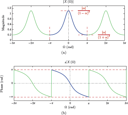
The magnitude and the phase of the transform are shown in Fig. 5.19(a) and (b) for the case α = 0.4.
![Figure showing the DTFT of the signal x[n] for Example 5.10 for α = 0.4: (a) the magnitude,](http://imgdetail.ebookreading.net/data/1/9781466598546/9781466598546__signals-and-systems__9781466598546__image__439x001.png)
Software resources:
ex_5_10.m
The demo program in “dtft_demo2.m” is based on Example 5.10. The signal x[n] is graphed along with the magnitude and the phase of its DTFT X (Ω). The parameter α may be varied, and its effects on the spectrum may be observed.
Software resources:
dtft_demo2.m
Example 5.11: DTFT of unit-impulse signal
Determine the DTFT of the unit-impulse signal x[n] = δ[n].
Solution: Direct application of Eqn. (5.71) yields
Using the sifting property of the impulse function, Eqn. (5.87) reduces to
Example 5.12: DTFT for discrete-time pulse
Determine the DTFT of the discrete-time pulse signal x[n] given by
Solution: Using Eqn. (5.71) the transform is
The closed form expression for a finite-length geometric series is (see Appendix C for derivation)
Using Eqn. (C.13) with a = e−jΩ, L1 = −L and L2 = L, the closed form expression for X (Ω) is
In order to get symmetric complex exponentials in Eqn. (5.89) we will multiply both the numerator and the denominator of the fraction on the right side of the equal sign with ejΩ/2. The result is
which, using Euler’s formula, can be simplified to
The value of the transform at Ω = 0 must be resolved through the use of L’Hospital’s rule:
The transform X (Ω) is graphed in Fig. 5.20 for L = 3, 4, 5.
![Figure showing the transform of the pulse signal x[n] of Example 5.12 for (a) L = 3, (b) L = 4, and (c) L = 5.](http://imgdetail.ebookreading.net/data/1/9781466598546/9781466598546__signals-and-systems__9781466598546__image__441x001.png)
The transform of the pulse signal x[n] of Example 5.12 for (a) L = 3, (b) L = 4, and (c) L = 5.
Software resources:
ex_5_12.m
The demo program in “dtft_demo3.m” is based on computing the DTFT of a discrete-time pulse explored in Example 5.12. The pulse with 2L + 1 unit-amplitude samples centered around n = 0 leads to the DTFT shown in Fig. 5.20. The demo program allows experimentation with that spectrum as L is varied.
Software resources:
dtft_demo3.m
Example 5.13: Inverse DTFT of rectangular spectrum
Determine the inverse DTFT of the transform X (Ω) defined in the angular frequency range −π< Ω <π by
Solution: To be a valid transform, X(Ω) must be 2π-periodic, therefore we need X(Ω) = X(Ω + 2π). The resulting transform is shown in Fig. 5.21.

The inverse x[n] is found by application of the DTFT synthesis equation given by Eqn. (5.70).
It should be noted that the expression found in Eqn. (5.90) for the signal x[n] is for all n; therefore, x[n] is non-causal. For convenience let us use the normalized frequency Fc related to the angular frequency Ωc by
and the signal x[n] becomes
The result is shown in Fig. 5.22 for the case Fc = 1/9. Zero crossings of the sinc function in Eqn. (5.91) are spaced 1/(2Fc) apart which has the non-integer value of 4.5 in this case. Therefore, the envelope of the signal x[n] crosses the axis at the midpoint of the samples for n = 4 and n = 5.
![Figure showing the signal x[n] for Example 5.13.](http://imgdetail.ebookreading.net/data/1/9781466598546/9781466598546__signals-and-systems__9781466598546__image__443x001.png)
Software resources:
ex_5_13.m
Interactive Demo: dtft_demo4
The demo program in “dtft_demo4.m” is based on Example 5.13 where the inverse DTFT of the rectangular spectrum shown in Fig. 5.21 was determined using the DTFT synthesis equation. The demo program displays graphs of the spectrum and the corresponding time-domain signal. The normalized cutoff frequency parameter Fc of the spectrum may be varied through the use of the slider control, and its effects on the signal x[n] may be observed. Recall that Ωc = 2πFc.
Software resources:
dtft_demo4.m
Example 5.14: Inverse DTFT of the unit-impulse function
Find the signal the DTFT of which is X(Ω) = δ(Ω) in the range −π< Ω <π.
Solution: To be a valid DTFT, the transform X(Ω) must be 2π-periodic. Therefore, the full expression for X(Ω) must be
as shown in Fig. 5.23.

The inverse transform is
Using the sifting property of the impulse function we get
Thus we have the DTFT pair
An important observation is in order: A signal that has constant amplitude for all index values is a power signal; it is neither absolute summable nor square summable. Strictly speaking, its DTFT does not converge. The transform relationship found in Eqn. (5.91) is a compromise made possible by our willingness to allow the use of singularity functions in X (Ω). Nevertheless, it is a useful relationship since it can be used in solving problems in the frequency domain.
Multiplying both sides of the relationship in Eqn. (5.91) by 2π results in
which is illustrated in Fig. 5.24. This relationship is fundamental, and will be explored further in the next example.
![Figure showing the constant signal x[n] = 1 and its transform X (Ω).](http://imgdetail.ebookreading.net/data/1/9781466598546/9781466598546__signals-and-systems__9781466598546__image__444x001.png)
Example 5.15: Inverse DTFT of impulse function revisited
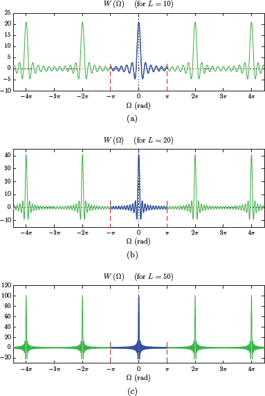
Consider again the DTFT transform pair found in Eqn. (5.92) of Example 5.14. The unit-amplitude signal x[n] = 1 can be thought of as the limit of the rectangular pulse signal explored in Example 5.12. Let
so that
Adapting from Example 5.12, the transform of w[n] is
and the transform of x[n] was found in Example 5.14 to be
Intuitively we would expect W(Ω) to resemble X(Ω) more and more closely as L is increased. Fig. 5.25 shows the transform W (Ω) for L = 10, 20, and 50. Observe the transition from W (Ω) to X (Ω) as L is increased.
Software resources:
ex_5_15.m
Interactive Demo: dtft_demo5
The demo program in “dtft_demo5.m” is based on Examples 5.14 and 5.15. The signal x[n] is a discrete-time pulse with 2L + 1 unit-amplitude samples centered around n = 0.
The parameter L may be varied. As L is increased, the signal x[n] becomes more and more similar to the constant amplitude signal of Example 5.14, and its spectrum approaches the spectrum shown in Fig. 5.24(b).
Software resources:
dtft_demo5.m
5.3.5 Properties of the DTFT
In this section we will explore some of the fundamental properties of the DTFT. As in the case of the Fourier transform for continuous-time signals, careful use of DTFT properties simplifies the solution of many types of problems.
Periodicity
The DTFT is periodic:
Periodicity of the DTFT is a direct consequence of the analysis equation given by Eqn. (5.71).
Linearity
DTFT is a linear transform.
For two transform pairs
and two arbitrary constants α1 and α2 it can be shown that
Proof: Use of the forward transform given by Eqn. (5.71) with the signal (α1x1[n] + α2x2[n]) yields
Time shifting
For a transform pair
it can be shown that
The consequence of shifting, or delaying, a signal in time is multiplication of its DTFT by a complex exponential function of angular frequency.
Proof: Applying the forward transform in Eqn. (5.71) to the signal x[n − m] we obtain
Let us apply the variable change k = n − m to the summation on the right side of Eqn. (5.97) so that
The exponential function in the summation of Eqn. (5.98) can be written as the product of two exponential functions to obtain
Example 5.16: DTFT of a time-shifted signal
Determine the DTFT of the signal x[n] = e−α(n−1) u[n − 1] as shown in Fig. 5.26. (Assume |α| < 1).
![Figure showing the signal x[n] for Example 5.16.](http://imgdetail.ebookreading.net/data/1/9781466598546/9781466598546__signals-and-systems__9781466598546__image__447x001.png)
Solution: The transform of a right-sided exponential signal was determined in Example 5.10.
As a result we have the transform pair
Applying the time shifting property of the DTFT given by Eqn. (5.96) with m = 1 leads to the result
Since |e−jΩ| = 1, the magnitude of X(Ω) is the same as that obtained in Example 5.10. Time shifting a signal does not change the magnitude of its transform.
The magnitude |X (Ω)| is shown in Fig. 5.27(a) for α = 0.4. The phase of X(Ω) is found by first determining the phase angles of the numerator and the denominator, and then subtracting the latter from the former. In Example 5.10 the numerator of the transform was a constant equal to unity; in this case it is a complex exponential. Therefore
![Figure showing the DTFT of the signal x[n] for Example 5.16 for α = 0.4: (a) the magnitude, (b) the phase as computed by Eqn. (5.100), (c) the phase shown in customary form.](http://imgdetail.ebookreading.net/data/1/9781466598546/9781466598546__signals-and-systems__9781466598546__image__448x001.png)
The DTFT of the signal x[n] for Example 5.16 for α = 0.4: (a) the magnitude, (b) the phase as computed by Eqn. (5.100), (c) the phase shown in customary form.
Thus, the phase of the transform differs from that obtained in Example 5.10 by −Ω, a ramp with a slope of −1. The phase, as computed by Eqn. (5.100), is shown in Fig. 5.27(b). In graphing the phase of the transform it is customary to fit phase values to in the range (−π, π) radians. Fig. 5.27(c) depicts the phase of the transform in the more traditional form.
Software resources:
ex_5_16.m
Interactive Demo: dtft_demo6
The demo program in “dtft_demo6.m” is based on Example 5.16. The signal
is shown along with the magnitude and the phase of its transform X (Ω). The time delay m can be varied, and its effect on the spectrum can be observed.
Observe that changing the amount of delay does not affect the magnitude of the spectrum.
Pay attention to the phase characteristic. In Example 5.16 we have used m = 1 and obtained the expression given by Eqn. (5.100) for the phase. When the signal is delayed by m samples the corresponding phase is
Software resources:
dtft_demo6.m
Time reversal
For a transform pair
it can be shown that
Time reversal of the signal causes angular frequency reversal of the transform. This property will be useful when we consider symmetry properties of the DTFT.
Proof: Direct application of the forward transform in Eqn. (5.71) to the signal x[−n] yields
Let us apply the variable change k = −n to the summation on the right side of Eqn. (5.102) to obtain
which can be written as
Example 5.17: DTFT of two-sided exponential signal
Determine the DTFT of the signal x[n] = α|n| with |α| < 1.
Solution: The signal x[n] can be written as
It can also be expressed as
where x1[n] is a causal signal and x2[n] is an anti-causal signal defined as
This is illustrated in Fig. 5.28.

(a) Two-sided exponential signal of Example 5.17, (b) its causal component, and (c) its anti-causal component.
Based on the linearity property of the DTFT, the transform of x[n] is the sum of the transforms of x1[n] and x2[n].
For the transform of x1 = αnu[n] we will make use of the result obtained in Example 5.10.
Time shifting and time reversal properties of the DTFT will be used for obtaining the transform of x2[n]. Let a new signal g[n] be defined as a scaled and time-shifted version of x1[n]:
Using the time shifting property, the transform of g[n] is
The signal x2[n] is a time reversed version of g[n], that is,
Applying the time reversal property, the transform of x2[n] is found as
Finally, X (Ω) is found by adding the two transforms:
The transform X(Ω) obtained in Eqn. (5.105) is real-valued, and is shown in Fig. 5.29 for α = 0.4.
![Figure showing the DTFT of the signal x[n] of Example 5.17 for a = 0.4.](http://imgdetail.ebookreading.net/data/1/9781466598546/9781466598546__signals-and-systems__9781466598546__image__452x001.png)
Software resources:
ex_5_17.m
Interactive Demo: dtft_demo7
The demo program in “dtft_demo7.m” is based on Example 5.17. It graphs the signal x[n] of Example 5.17 and the corresponding spectrum which is purely real due to the even symmetry of the signal. Parameter α can be varied in order to observe its effect on the spectrum.
Software resources:
dtft_demo7.m
Conjugation property
For a transform pair
it can be shown that
Conjugation of the signal causes both conjugation and angular frequency reversal of the transform. This property will also be useful when we consider symmetry properties of the DTFT.
Proof: Using the signal x*[n] in the forward transform equation results in
Writing the right side of Eqn. (5.107) in a slightly modified form we obtain
Symmetry of the DTFT
If the signal x[n] is real-valued, it can be shown that its DTFT is conjugate symmetric. Conversely, if the signal x[n] is purely imaginary, its transform is conjugate antisymmetric.
Symmetry of the DTFT:
Proof:
Real x(t):
Any real-valued signal is equal to its own conjugate, therefore we have
Taking the transform of each side of Eqn. (5.111) and using the conjugation property stated in Eqn. (5.106) we obtain
which is equivalent to Eqn. (5.109).
Imaginary x(t):
A purely imaginary signal is equal to the negative of its conjugate, i.e.,
Taking the transform of each side of Eqn. (5.113) and using the conjugation property given by Eqn. (5.106) yields
This is equivalent to Eqn. (5.110). Therefore the transform is conjugate antisymmetric.
Cartesian and polar forms of the transform
A complex transform X(Ω) can be written in polar form as
and in Cartesian form as
Case 1: If X (Ω) is conjugate symmetric, the relationship in Eqn. (5.109) can be written as
using the polar form of the transform, and
using its Cartesian form. The consequences of Equation (5.117) Equation (5.118) can be obtained by equating the magnitudes and the phases on both sides of Eqn. (5.117) and by equating real and imaginary part on both sides of Eqn. (5.118). The results are summarized below:
Conjugate symmetric transform:
The transform of a real-valued x[n] is conjugate symmetric. For such a transform, the magnitude is an even function of Ω, and the phase is an odd function. Furthermore, the real part of the transform has even symmetry, and its imaginary part has odd symmetry.
Case 2: If X(Ω) is conjugate antisymmetric, the polar form of X(Ω) has the property
The negative sign on the right side of Eqn. (5.123) needs to be incorporated into the phase since we could not write |X(−Ω)| = −|X(Ω)| (recall that magnitude needs to be a non-negative function for all Ω). Using e∓jπ = −1, Eqn. (5.123) can be written as
Conjugate antisymmetry property of the transform can also be expressed in Cartesian form as
The consequences of Equation (5.124) and Equation (5.125) are given below.
Conjugate antisymmetric transform:
We know that a purely-imaginary signal leads to a DTFT that is conjugate antisymmetric. For such a transform the magnitude is still an even function of Ω as suggested by Eqn. (5.126). The phase is neither even nor odd. The real part is an odd function of Ω, and the imaginary part is an even function.
Transforms of even and odd signals
If the real-valued signal x[n] is an even function of time, the resulting transform X(Ω) is real-valued for all Ω.
Proof: Using the time reversal property of the DTFT, Eqn. (5.130) implies that
Furthermore, since x[n] is real-valued, the transform is conjugate symmetric, therefore
Combining Equation (5.131) and Equation (5.132) we reach the conclusion
Therefore, X (Ω) must be real.
Conversely it can also be proven that, if the real-valued signal x[n] has odd-symmetry, the resulting transform is purely imaginary. This can be stated mathematically as follows:
Conjugating a purely imaginary transform is equivalent to negating it, so an alternative method of expressing the relationship in Eqn. (5.134) is
Proof of Eqn. (5.135) is similar to the procedure used above for proving Eqn. (5.130) (see Problem 5.14 at the end of this chapter).
Frequency shifting
For a transform pair
it can be shown that
Modulation property
For a transform pair
it can be shown that
and
Modulation property is an interesting consequence of the frequency shifting property combined with the linearity of the Fourier transform. Multiplication of a signal by a cosine waveform causes its spectrum to be shifted in both directions by the angular frequency of the cosine waveform, and to be scaled by . Multiplication of the signal by a sine waveform causes a similar effect with an added phase shift of −π/2 radians for positive frequencies and π/2 radians for negative frequencies.
Proof: Using Euler’s formula, the left side of the relationship in Eqn. (5.138) can be written as
The desired proof is obtained by applying the frequency shifting theorem to the terms on the right side of Eqn. (5.140). Using Eqn. (5.136) we obtain
and
which could be used together in Eqn. (5.140) to arrive at the result in Eqn. (5.138).
The proof of Eqn. (5.139) is similar, but requires one additional step. Again using Euler’s formula, let us write the left side of Eqn. (5.139) as
Eqn. (5.143) can be rewritten as
The proof of Eqn. (5.139) can be completed by using Equation (5.141) and Equation (5.142) on the right side of Eqn. (5.144).
Differentiation in the frequency domain
For a transform pair
it can be shown that
and
Proof: Differentiating both sides of Eqn. (5.71) with respect to Ω yields
The summation on the right side of Eqn. (5.147) is the DTFT of the signal −jn x[n]. Multiplying both sides of Eqn. (5.147) by j results in the transform pair in Eqn. (5.145). Eqn. (5.146) is proven by repeated use of Eqn. (5.145).
Example 5.18: Use of differentiation in frequency property
Determine the DTFT of the signal x[n] = ne−αn u[n] shown in Fig. 5.30. Assume |α| < 1.
![Figure showing the signal x[n] for Example 5.18.](http://imgdetail.ebookreading.net/data/1/9781466598546/9781466598546__signals-and-systems__9781466598546__image__457x001.png)
Solution: In Example 5.10 we have established the following transform pair:
Applying the differentiation in frequency property of the DTFT leads to
Differentiation is carried out easily:
and the transform we seek is
The magnitude and the phase of the transform X(Ω) are shown in Fig. 5.31(a) and (b) for the case α = 0.4.
Software resources:
ex_5_18.m
Convolution property
For two transform pairs
it can be shown that
Convolving two signals in the time domain corresponds to multiplying the corresponding transforms in the frequency domain.
Proof: The convolution of signals x1[n] and x2[n] is given by
Using Eqn. (5.149) in the DTFT definition yields
Changing the order of the two summations in Eqn. (5.150) and rearranging terms we obtain
In Eqn. (5.151) the expression in square brackets should be recognized as the transform of time-shifted signal x2[n − k], and is equal to X2(Ω) e−jΩk. Using this result in Eqn. (5.151) leads to
Example 5.19: Convolution using the DTFT
Two signals are given as
Determine the convolution y[n] = h[n] * x[n] of these two signals using the DTFT.
Solution: Transforms of H(Ω) and X(Ω) can easily be found using the result obtained in Example 5.10:
Using the convolution property, the transform of y[n] is
The transform Y(Ω) found in Eqn. (5.153) can be written in the form
The convolution result y[n] is the inverse DTFT of Y(Ω) which can be obtained using the linearity property of the transform:
Solution of problems of this type will be more practical through the use of z-transform in Chapter 8.
Software resources:
ex_5_19.m
Multiplication of two signals
For two transform pairs
it can be shown that
The DTFT of the product of two signals x1[n] and x2[n] is equal the 2π-periodic convolution of the individual transforms X1(Ω) and X2(Ω).
Proof: Applying the DTFT definition to the product x1[n] x2[n] leads to
Using the DTFT synthesis equation given by Eqn. (5.70) we get
Substituting Eqn. (5.157) into Eqn. (5.156)
Interchanging the order of summation and integration, and rearranging terms yields
Table 5.3 contains a summary of key properties of the DTFT. Table 5.4 lists some of the fundamental DTFT pairs.
DTFT properties.
Theorem |
Signal |
Transform |
Linearity |
αx1[n] + βx2[n] |
αX1 (Ω) + βX2 (Ω) |
Periodicity |
x[n] |
X (Ω) = X (Ω + 2πr) for all integers r |
Conjugate symmetry |
x[n] real |
X* (Ω) = X (−Ω) |
|
|
Magnitude: |X (−Ω)| = |X (Ω)| |
|
|
Phase: Θ (−Ω) = −Θ(Ω) |
|
|
Real part: Xr (−Ω) = Xr (Ω) |
|
|
Imaginary part: Xi (−Ω) = −Xi (Ω) |
Conjugate antisymmetry |
x[n] imaginary |
X* (Ω) = −X (−Ω) |
|
|
Magnitude: |X (−Ω)| = |X (Ω)| |
|
|
Phase: Θ (−Ω) = −Θ(Ω) ∓ π |
|
|
Real part: Xr (−Ω) = −Xr (Ω) |
|
|
Imaginary part: Xi (−Ω) = Xi (Ω) |
Even signal |
x[n] = x[−n] |
Im {X (Ω)} = 0 |
Odd signal |
x[n] = −x[−n] |
Re {X (Ω)} = 0 |
Time shifting |
x[n − m] |
X(Ω) e−jΩm |
Time reversal |
x[−n] |
X(−Ω) |
Conjugation |
x*[n] |
X* (−Ω) |
Frequency shifting |
x[n] ejΩ0n |
X(Ω − Ω0) |
Modulation |
x[n] cos(Ω0n) |
|
|
x[n] sin(Ω0n) |
|
Differentiation in frequency |
nmx[n] |
|
Convolution |
x1[n] * x2[n] |
X1 (Ω) X2 (Ω) |
Multiplication |
x1[n]x2[n] |
|
Parseval’s theorem |
||
Some DTFT transform pairs.
Name |
Signal |
Transform |
Discrete-time pulse |
||
Unit-impulse signal |
x[n] = δ[n] |
X (Ω) = 1 |
Constant-amplitude signal |
x[n] = 1, all n |
|
Sinc function |
||
Right-sided exponential |
x[n] = αnu[n] , |α| < 1 |
|
Complex exponential |
x[n] = ejΩ0n |
5.3.6 Applying DTFT to periodic signals
In previous sections of this chapter we have distinguished between two types of discrete-time signals: periodic and non-periodic. For periodic discrete-time signals we have the DTFS as an analysis and problem solving tool; for non-periodic discrete-time signals the DTFT serves a similar purpose. This arrangement will serve us adequately in cases where we work with one type of signal or the other. There may be times, however, when we need to mix periodic and non-periodic signals within one system. For example, in amplitude modulation, a non-periodic signal may be multiplied with a periodic signal, and we may need to analyze the resulting product in the frequency domain. Alternately, a periodic signal may be used as input to a system the impulse response of which is non-periodic. In these types of scenarios it would be convenient to find a way to use the DTFT for periodic signals as well. We have seen in Example 5.14 that a DTFT can be found for a constant-amplitude signal that does not satisfy the existence conditions, as long as we are willing to accept singularity functions in the transform. The next two examples will expand on this idea. Afterwards we will develop a technique for converting the DTFS of any periodic discrete-time signal to a DTFT.
Example 5.20: DTFT of complex exponential signal
Determine the transform of the complex exponential signal x[n] = ejΩ0n with −π < Ω0 < π.
Solution: The transform of the constant unit-amplitude signal was found in Example 5.14 to be
Using this result along with the frequency shifting property of the DTFT given by Eqn. (5.136), the transform of the complex exponential signal is
This is illustrated in Fig. 5.32.
![Figure showing the transform of complex exponential signal x[n] = ejΩ0n.](http://imgdetail.ebookreading.net/data/1/9781466598546/9781466598546__signals-and-systems__9781466598546__image__463x001.png)
Example 5.21: DTFT of sinusoidal signal
Determine the transform of the sinusoidal signal x[n] = cos(Ω0n) with −π < Ω0 < π.
Solution: The transform of the constant unit-amplitude signal was found in Example 5.14 to be
Using this result along with the modulation property of the DTFT given by Eqn. (5.138), the transform of the sinusoidal signal is
Let represent the part of the transform in the range −π < Ω < π.
The DTFT can now be expressed as
This is illustrated in Fig. 5.33.
![Figure showing the transform of complex exponential signal x[n] = cos(Ω0n): (a) the middle part ¯X (Ω), (b) the complete transform X (Ω).](http://imgdetail.ebookreading.net/data/1/9781466598546/9781466598546__signals-and-systems__9781466598546__image__463x002.png)
The transform of complex exponential signal x[n] = cos(Ω0n): (a) the middle part ¯X (Ω), (b) the complete transform X (Ω).
In Examples 5.20 and 5.21 we were able to obtain the DTFT of two periodic signals, namely a complex exponential signal and a sinusoidal signal. The idea can be generalized to apply to any periodic discrete-time signal. The DTFS synthesis equation for a periodic signal was given by Eqn. (5.21) which is repeated here for convenience:
If we were to attempt to find the DTFT of the signal by direct application of the DTFT analysis equation given by Eqn. (5.71) we would need to evaluate
Substituting Eqn. (5.21) into Eqn. (5.164) leads to
Interchanging the order of the two summations in Eqn. (5.165) and rearranging terms we obtain
In Eqn. (5.166) the expression in square brackets is the DTFT of the signal ej(2π/N)kn. Using the result obtained in Example 5.20, and remembering that 2π/N = Ω0 is the fundamental angular frequency for the periodic signal , we get
and
The part of the transform in the range 0 < Ω < 2π is found by setting m = 0 in Eqn. (5.168):
Thus, for a periodic discrete-time signal is obtained by converting each DTFS coefficient to an impulse with area equal to 2π and placing it at angular frequency Ω = kΩ0. The DTFT for the signal is then obtained as
This process is illustrated in Fig. 5.34.
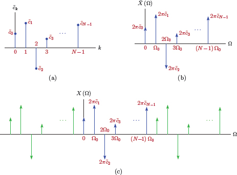
(a) DTFS coefficients for a signal periodic with N, (b) DTFT for −π < Ω < π, (c) complete DTFT.
Note: In Eqn. (5.162) of Example 5.21 we have used to represent the part of the transform in the range −π < Ω < π. On the other hand, in Eqn. (5.169) above, was used as the part of the transform in the range 0 < Ω < 2π. This should not cause any confusion. In general, represents one period of the 2π-periodic transform, and the starting value of Ω is not important.
Example 5.22: DTFT of the periodic signal of Example 5.4
Determine the DTFT of the signal x[n] used in Example 5.4 and shown in Fig. 5.3.
Solution: We will first write the transform in the interval 0 < Ω < 2π.
The period of the signal is N = 5, therefore the fundamental angular frequency is Ω0 = 2π/5. Using the values of DTFS coefficients found in Example 5.4 we obtain
The complete transform X (Ω) is found by periodically extending .
5.4 Energy and Power in the Frequency Domain
Parseval’s theorem and its application to the development of energy and power spectral density concepts were discussed for continuous-time signals in Section 4.4 of Chapter 4. In this section we will discuss Parseval’s theorem for periodic and non-periodic discrete-time signals, and introduce the corresponding energy and power spectral density concepts.
5.4.1 Parseval’s theorem
For a periodic power signal with period N and DTFS coefficients it can be shown that
For a non-periodic energy signal x[n] with DTFT X(Ω), the following holds true:
The left side of Eqn. (5.173) represents the normalized average power in a periodic signal which was derived in Chapter 1 Eqn. (1.187). The left side of Eqn. (5.174) represents the normalized signal energy as derived in Eqn. (1.180). The relationships given by Equation (5.173) and Equation (5.174) relate signal energy or signal power to the frequency-domain representation of the signal. They are two forms of Parseval’s theorem.
Proofs: First we will prove Eqn. (5.173). DTFS representation of a periodic discrete-time signal with period N was given by Eqn. (5.21), and is repeated here for convenience:
Using |x[n]|2 = x[n] x*[n], the left side of Eqn. (5.173) can be written as
Rearranging the order of the summations in Eqn. (5.175) we get
Using orthogonality of the basis function set {ej(2π/N)kn, k = 0,...,N − 1 it can be shown that (see Appendix D)
Using Eqn. (5.177) in Eqn. (5.176) leads to the desired result:
The proof for Eqn. (5.174) is similar. The DTFT synthesis equation was given by Eqn. (5.70) and is repeated here for convenience.
The left side of Eqn. (5.174) can be written as
Interchanging the order of the integral and the summation in Eqn. (5.179) and rearranging terms yields
5.4.2 Energy and power spectral density
The two statements of Parseval’s theorem given by Equation (5.173) and Equation (5.174) lead us to the following conclusions:
In Eqn. (5.173) the left side corresponds to the normalized average power of the periodic signal , and therefore the summation on the right side must also represent normalized average power. The term corresponds to the power of the signal component at angular frequency Ω = kΩ0. (Remember that Ω0 = 2π/N.) Let us construct a new function Sx (Ω) as follows:
The function Sx (Ω) consists of impulses placed at angular frequencies kΩ0 as illustrated in Fig. 5.35. Since the DTFS coefficients are periodic with period N, the function Sx(Ω) is 2π-periodic.
Integrating Sx (Ω) over an interval of 2π radians leads to
Interchanging the order of integration and summation in Eqn. (5.182) and rearranging terms we obtain
Recall that Ω0 = 2π/N. Using the sifting property of the impulse function, the integral between square brackets in Eqn. (5.183) is evaluated as
and Eqn. (5.183) becomes
The normalized average power of the signal is therefore found as
Consequently, the function Sx (Ω) is the power spectral density of the signal . Since Sx (Ω) is 2π-periodic, the integral in Eqn. (5.186) can be started at any value of Ω as long as it covers a span of 2π radians. It is usually more convenient to write the integral in Eqn. (5.186) to start at −π.
As an interesting by-product of Eqn. (5.186), the normalized average power of that is within a specific angular frequency range can be determined by integrating Sx (Ω) over that range. For example, the power contained at angular frequencies in the range (−Ω0, Ω0) is
In Eqn. (5.174) the left side is the normalized signal energy for the signal x[n], and the right side must be the same. The integrand |X (Ω)|2 is therefore the energy spectral density of the signal x[n]. Let the function Gx (Ω) be defined as
Substituting Eqn. (5.189) into Eqn. (5.174), the normalized energy in the signal x[n] can be expressed as
The energy contained at angular frequencies in the range (−Ω0, Ω0) is found by integrating Gx (Ω) in the frequency range of interest:
In Eqn. (5.174) we have expressed Parseval’s theorem for an energy signal, and used it to lead to the derivation of the energy spectral density in Eqn. (5.189). We know that some non-periodic signals are power signals, therefore their energy cannot be computed. The example of one such signal is the unit-step function. The power of a non-periodic signal was defined in Eqn. (1.188) in Chapter 1 which will be repeated here:
In order to write the counterpart of Eqn. (5.174) for a power signal, we will first define a truncated version of x[n] as
Let XT (Ω) be the DTFT of the truncated signal xT [n]:
Now Eqn. (5.174) can be written in terms of the truncated signal and its transform as
Scaling both sides of Eqn. (5.194) by (2M + 1) and taking the limit as M becomes infinitely large, we obtain
The left side of Eqn. (5.195) is the average normalized power in a non-periodic signal as we have established in Eqn. (1.188). Therefore, the power spectral density of x[n] is
![Figure showing the function Sx (Ω) constructed using the DTFS coefficents of the signal x˜[n].](http://imgdetail.ebookreading.net/data/1/9781466598546/9781466598546__signals-and-systems__9781466598546__image__468x001.png)
Example 5.23: Normalized average power for waveform of Example 5.7
Consider again the periodic waveform used in Example 5.7 and shown in Fig. 5.6. Using the DTFS coefficients found in Example 5.7, verify Parseval’s theorem. Also determine the percentage of signal power in the angular frequency range −π/3 < Ω0 <π/3.
Solution: The average power computed from the signal is
Using the DTFS coefficients in Table 5.1 yields
As expected, the value found from DTFS coefficients matches that found from the signal. One period of the power spectral density Sx (Ω) is
The power in the angular frequency range of interest is
The ratio of the power in −π/3 < Ω0 <π/3 to the total signal power is
It appears that 97.9 percent of the power of the signal is in the frequency range −π/3 < Ω0 <π/3.
Software resources:
ex_5_23.m
Example 5.24: Power spectral density of a discrete-time sinusoid
Find the power spectral density of the signal
Solution: Using Euler’s formula, the signal can be written as
The normalized frequency of the sinusoidal signal is F0 = 0.1 corresponding to a period length of N = 10 samples. Non-zero DTFS coefficients for k = 0,..., 9 are
Using Eqn. (5.181), the power spectral density is
which is shown in Fig. 5.36.
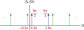
The power in the sinusoidal signal is computed from the power spectral density as
Example 5.25: Energy spectral density of a discrete-time pulse
Determine the energy spectral density of the rectangular pulse
Also compute the energy of the signal in the frequency interval −π/10 < Ω <π/10.
Solution: Using the general result obtained in Example 5.12 with L = 5, the DTFT of the signal x[n] is
The energy spectral density for x[n] is found as
which is shown in Fig. 5.37.
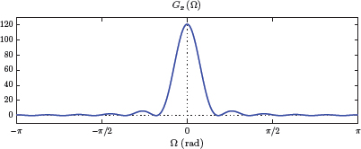
The energy of the signal within the frequency interval −π/10 < Ω <π/10 is computed as
which is proportional to the shaded area under G (Ω) in Fig. 5.38.

Direct evaluation of the integral in Eqn. (5.197) is difficult; however, the result can be obtained by numerical approximation of the integral, and is
Software resources:
ex_5_25.m
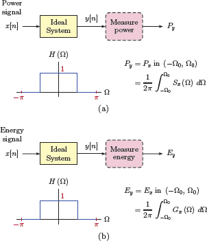
Energy or power in a frequency range
Signal power or signal energy that is within a finite range of frequencies is found through the use of Equation (5.188) and Equation (5.191) respectively. An interesting interpretation of the result in Eqn. (5.188) is that, for the case of a power signal, the power of x[n] in the frequency range −Ω0 < Ω < Ω0 is the same as the power of the output signal of a system with system function
driven by the signal x[n]. Similarly, for the case of an energy signal, the energy of x[n] in the frequency range −Ω0 < Ω < Ω0 is the same as the energy of the output signal of a system with the system function in Eqn. (5.197) driven by the signal x[n]. These relationships are illustrated in Fig. 5.39(a) and (b).
5.4.3 Autocorrelation
The energy spectral density Gx (Ω) or the power spectral density Sx (Ω) for a signal can be computed through direct application of the corresponding equations derived in Section 5.4.2; namely Eqn. (5.189) for an energy signal, and either Eqn. (5.181) or Eqn. (5.196) for a power signal, depending on its type. In some circumstances it is also possible to compute either function from the knowledge of the autocorrelation function which will be defined in this section. Let x[n] be a real-valued signal.
For an energy signal x[n] the autocorrelation function is defined as
For a periodic power signal with period N, the corresponding definition of the autocorrelation function is
The triangle brackets indicate time average. The autocorrelation function for a periodic signal is also periodic as signified by the tilde (˜) character used over the symbol rxx in Eqn. (5.199). Finally, for a non-periodic power signal, the corresponding definition is
Even though we refer to rxx[m] as a function, we will often treat it as if it is a discrete-time signal, albeit one that uses a different index, m, from the signal x[n] for which it is computed. The index m simply corresponds to the time shift between the two copies of x[n] used in the definitions of Equation (5.198) through Equation (5.200).
It can be shown that, for an energy signal, the energy spectral density is the DTFT of the autocorrelation function, that is,
Proof: Let us begin by applying the DTFT definition to the autocorrelation function rxx[m] treated as a discrete-time signal indexed by m:
The two summations in Eqn. (5.202) can be rearranged to yield
Realizing that the inner summation in Eqn. (5.203) is equal to
Eqn. (5.203) becomes
and since x[n] is real, we obtain
which completes the proof.
The definition of the autocorrelation function for a periodic signal can be used in a similar manner in determining the power spectral density of the signal.
Let the signal and the autocorrelation function , both periodic with period N, have the DTFS representations given by
and
respectively. It can be shown that the DTFS coefficients and are related by
and the power spectral density is the DTFT of the autocorrelation function, that is,
Proof: Using the DTFS analysis equation given by Eqn. (5.22) with the definition of the autocorrelation function in Eqn. (5.199) leads to
Rearranging the order of the two summations Eqn. (5.211) can be written as
Using the time shifting property of the DTFS given by Eqn. (5.30) the expression in square brackets in Eqn. (5.212) is
Substituting Eqn. (5.213) into Eqn. (5.212) yields
Using the technique developed in Section 5.3.6 the DTFT of is
Using Eqn. (5.214) in Eqn. (5.215) results in
which is identical to the expression given by Eqn. (5.181) for the power spectral density of a periodic signal.
A relationship similar to the one expressed by Eqn. (5.210) applies to random processes that are wide-sense stationary, and is known as the Wiener-Khinchin theorem. It is one of the fundamental theorems of random signal processing.
Example 5.26: Power spectral density of a discrete-time sinusoid revisited
Consider again the discrete-time sinusoidal signal
the power spectral density of which was determined in Example 5.24. Determine the autocorrelation function for this signal, and then find the power spectral density Sx (Ω) from the autocorrelation function.
Solution: The period of is N = 10 samples. Using the definition of the autocorrelation function for a periodic signal
Through the use of the appropriate trigonometric identity, the result in Eqn. (5.217) is simplified to
In Eqn. (5.218) the first summation is equal to zero since its term cos (0.4πn +0.2πm) is periodic with a period of five samples, and the summation is over two full periods. The second summation yields
for the autocorrelation function. The power spectral density is found as the DTFT of the autocorrelation function. Application of the DTFT was discussed in Section 5.3.6. Using the technique developed in that section (specifically see Example 5.21) the transform is found as
which matches the answer found earlier in Example 5.24.
Software resources:
ex_5_26.m
Properties of the autocorrelation function
The autocorrelation function as defined by Equation (5.198), Equation (5.199) and Equation (5.200) has a number of important properties that will be summarized here:
rxx[0] ≥ |rxx[m]| for all m.
To see why this is the case, we will consider the non-negative function (x[n] ∓ x[n + m])2.
The time average of this function must also be non-negative, therefore
or equivalently
which implies that
which is the same as property 1.
rxx[−m] = rxx[m] for all m, that is, the autocorrelation function has even symmetry. Recall that the autocorrelation function is the inverse Fourier transform of either the energy spectral density or the power spectral density. Since Gx (Ω) and Sx (Ω) are purely real, rxx[m] must be an even function of m.
If the signal is periodic with period N, then its autocorrelation function is also periodic with the same period. This property easily follows from the time-average based definition of the autocorrelation function given by Eqn. (5.199).
5.5 System Function Concept
In time-domain analysis of systems in Chapter 3 two distinct description forms were used for DTLTI systems:
- A linear constant-coefficient difference equation that describes the relationship between the input and the output signals
- An impulse response which can be used with the convolution operation for determining the response of the system to an arbitrary input signal
In this section, the concept of system function will be introduced as the third method for describing the characteristics of a system.
The system function is simply the DTFT of the impulse response:
Recall that the impulse response is only meaningful for a system that is both linear and time-invariant (since the convolution operator could not be used otherwise). It follows that the system function concept is valid for linear and time-invariant systems only. In general, H (Ω) is a complex function of Ω, and can be written in polar form as
Obtaining the system function from the difference equation
In finding a system function for a DTLTI system described by means of a difference equation, two properties of the DTFT will be useful: the convolution property and the time shifting property.
Since the output signal is computed as the convolution of the impulse response and the input signal, that is, y[n] = h[n] * x[n], the corresponding relationship in the frequency domain is Y (Ω) = H (Ω) X (Ω). Consequently, the system function is equal to the ratio of the output transform to the input transform:
Using the time shifting property, transforms of the individual terms in the difference equation are found as
The system function is obtained from the difference equation by first transforming both sides of the difference equation through the use of Equation (5.222) and Equation (5.223), and then using Eqn. (5.221).
Example 5.27: Finding the system function from the difference equation
Determine the system function for a DTLTI system described by the difference equation
Solution: Taking the DTFT of both sides of the difference equation we obtain
which can be written as
The system function is found through the use of Eqn. (5.221)
The magnitude and the phase of the system function are shown in Fig. 5.40.

Software resources:
ex_5_27.m
Example 5.28: System function for length-N moving average filter
Recall the length-N moving average filter with the difference equation
Determine the system function. Graph its magnitude and phase as functions of Ω.
Solution: Taking the DTFT of both sides of the difference equation we obtain
from which the system function is found as
The expression in Eqn. (5.224) can be put into closed form as
As the first step in expressing H (Ω) in polar complex form, we will factor out e−jΩN/2 from the numerator and e−jΩ/2 from the denominator to obtain
The magnitude and the phase of the system function are shown in Fig. 5.41 for N = 4.

ex_5_28.m
Interactive Demo: sf_sdemo5.m
The demo program in “sf_demo5.m” is based on Example 5.28. It computes and graphs the magnitude and the phase of the system function H (Ω) for the length-N moving average filter. The filter length N may be varied.
- Observe that zero crossings (dips) of the magnitude spectrum divide the angular frequency interval 0 ≤ Ω ≤ 2π into N equal segments.
- Pay attention to the phase of the system function. Its sloped sections all have the same slope, indicating that the phase response is linear. How does the slope of the phase response relate to the filter length N?
Software resources:
sf_demo5.m
5.6 DTLTI Systems with Periodic Input Signals
In earlier sections of this chapter we have explored the use of the discrete-time Fourier series (DTFS) for representing periodic discrete-time signals. It was shown that a periodic discrete-time signal can be expressed using complex exponential basis functions in the form
If a periodic signal is used as input to a DTLTI system, the use of the superposition property allows the response of the system to be determined as a linear combination of its responses to individual basis functions
5.6.1 Response of a DTLTI system to complex exponential signal
Consider a DTLTI system with impulse response h[n], driven by a complex exponential input signal
The response y[n] of the system is found through the use of the convolution relationship that was derived in Section 3.7.2 of Chapter 3.
Using the signal given by Eqn. (5.225) in Eqn. (5.226) we get
or, equivalently
The summation in Eqn. (5.228) should be recognized as the system function evaluated at the specific angular frequency Ω = Ω0. Therefore
We have used the tilde (˜) character over the name of the output signal in realization of the fact that it is also periodic. The development in Equation (5.227) through Equation (5.229) is based on the inherent assumption that the Fourier transform of h[n] exists. This in turn requires the corresponding DTLTI system to be stable. Any natural response the system may have exhibited at one point would have disappeared a long time ago. Consequently, the response found in Eqn. (5.229) is the steady-state response of the system.
For a DTLTI system driven by a complex exponential input signal, we have the following important relationship:
Response to complex exponential input:
- The response of a DTLTI system to a complex exponential input signal is a complex exponential output signal with the same angular frequency Ω0.
- The effect of the system on the complex exponential input signal is to
- Scale its amplitude by an amount equal to the magnitude of the system function at Ω = Ω0
- Shift its phase by an amount equal to the phase of the system function at Ω = Ω0
5.6.2 Response of a DTLTI system to sinusoidal signal
Let the input signal to the DTLTI system under consideration be a sinusoidal signal in the form
The response of the system in this case will be determined by making use of the results of the previous section.
We will use Euler’s formula to write the input signal using two complex exponential functions as
This representation of allows the results of the previous section to be used. The output signal can be written using superposition:
If the impulse response h[n] is real-valued, the result in Eqn. (5.233) can be further simplified. Recall from Section 5.3.5 that, for real-valued h[n], the transform H (Ω) is conjugate symmetric, resulting in
Using these relationships, Eqn. (5.233) becomes
For a DTLTI system driven by a cosine input signal, we have the following important relationship:
Response to cosine input:
- When a DTLTI system is driven by single-tone input signal at angular frequency Ω0, its output signal is also a single-tone signal at the same angular frequency.
- The effect of the system on the input signal is to
- Scale its amplitude by an amount equal to the magnitude of the system function at Ω = Ω0
- Shift its phase by an amount equal to the phase of the system function at Ω = Ω0
Example 5.29: Steady-state response of DTLTI system to sinusoidal input
Consider a DTLTI system characterized by the difference equation
The system function for this system was determined in Example 5.27 to be
Find the response of the system to the sinusoidal input signal
Solution: Evaluating the system function at the angular frequency Ω0 = π/5 yields
which can be written in polar form as
The magnitude and the phase of the system function are shown in Fig. 5.42. The values of magnitude and phase at the angular frequency of interest are marked on the graphs.

The steady-state response of the system to the specified input signal is
Software resources:
ex_5_29.m
See MATLAB Exercise 5.4. |
Interactive Demo: sf_demo6.m
The demo program “sf_demo6.m” is based on Example 5.29. It computes and graphs the steady-state response of the system under consideration to the sinusoidal input signal
The normalized frequency F0 can be varied from F0 = 0.01 to F0 = 0.49 using a slider control. As F0 is varied, the display is updated
- To show the changes to the steady-state response
- To show the critical magnitude and phase and values on the graphs of the system function
Software resources:
sf_demo6.m
5.6.3 Response of a DTLTI system to periodic input signal
Using the development in the previous sections, we are now ready to consider the use of a general periodic signal as input to a DTLTI system. Using the DTFS representation of the signal, the response of the system is
Let us use the linearity of the system to write the response as
Based on Eqn. (5.230) the response of the system to an exponential basis function at frequency Ω = 2πk/N is given by
Using Eqn. (5.239) in Eqn. (5.238), the response of the system to is found as
Two important observations should be made based on Eqn. (5.240):
- For a DTLTI system driven by an input signal with period N, the output signal is also periodic with the same period.
- If the DTFS coefficients of the input signal are then the DTFS coefficients of the output signal are such that
Example 5.30: Response of DTLTI system to discrete-time sawtooth signal
Let the discrete-time sawtooth signal used in Example 5.4 and shown again in Fig. 5.43 be applied to the system with system function
![Figure showing the signal x˜[n] for Example 5.30.](http://imgdetail.ebookreading.net/data/1/9781466598546/9781466598546__signals-and-systems__9781466598546__image__486x001.png)
Find the steady-state response of the system.
Solution: The DTFS coefficients for were determined in Example 5.4, and are repeated below:
Evaluating the system function at angular frequencies
we obtain
The DTFS coefficients for the output signal are found using Eqn. (5.241):
The output signal y[n] can now be constructed using the DTFS coefficients :
and is shown in Fig. 5.44.
![Figure showing the output signal ˜ y[n] for Example 5.30.](http://imgdetail.ebookreading.net/data/1/9781466598546/9781466598546__signals-and-systems__9781466598546__image__487x001.png)
Software resources:
ex_5_30.m
5.7 DTLTI Systems with Non-Periodic Input Signals
Let us consider the case of using a non-periodic signal x[n] as input to a DTLTI system. It was established in Section 3.7.2 of Chapter 3 that the output of a DTLTI system is equal to the convolution of the input signal with the impulse response, that is
Let us assume that
We have seen in Section 5.3.5 of this chapter that the DTFT of the convolution of two signals is equal to the product of individual transforms:
The output transform is the product of the input transform and the system function.
Writing each transform involved in Eqn. (5.243) in polar form using its magnitude and phase we obtain the corresponding relationships:
- The magnitude of the output spectrum is equal to the product of the magnitudes of the input spectrum and the system function.
- The phase of the output spectrum is found by adding the phase characteristics of the input spectrum and the system function.
5.8 Discrete Fourier Transform
In previous sections of this chapter we have studied the discrete-time Fourier series (DTFS) for periodic discrete-time signals, and the discrete-time Fourier transform (DTFT) for non-periodic discrete-time signals. The result of DTFT analysis of a discrete-time signal x[n] is a transform X (Ω) which, if it exists, is a 2π-periodic function of the continuous variable Ω. Storing the DTFT of a signal on a digital computer is impractical because of the continuous nature of Ω. On the other hand, the DTFS representation of a signal that is periodic with N samples is a set of coefficients that is also periodic with N. While this combination would certainly be suitable for computer implementation and storage, it is only for periodic signals. We often deal with signals that are not necessarily periodic.
In the analysis of non-periodic discrete-time signals, sometimes it is desirable to have a transform that is also discrete. This can be accomplished through the use of the discrete Fourier transform (DFT) provided that the signal under consideration is finite-length.
Consider a signal x[n] the meaningful samples of which are limited to the index range n = 0,...,N − 1, that is,
We will refer to x[n] as a length-N signal since it has N non-trivial samples. An easy method of representing x[n] with a transform that is also length-N would be as follows:
Consider x[n] as one period of a periodic signal defined as
We will refer to as the periodic extension of x[n].
Determine the DTFS coefficients for the periodic extension obtained from x[n] through Eqn. (5.246):
DTFS coefficients of form a set that is also periodic with N. Let us extract just one period {ck; k = 0,...,N − 1} from the DTFS coefficients {;all k}:
This gives us the ability to represent the signal x[n] with the set of coefficients ck for k = 0,...,N − 1. The coefficients can be obtained from the signal using the three steps outlined above. Conversely, the signal can be reconstructed from the coefficients by simply reversing the order of the steps.
The discrete Fourier transform (DFT) will be defined by slightly modifying the idea presented above. The forward transform is
The length-N signal x[n] leads to the length-N transform X[k]. Compare Eqn. (5.249) with DTFS analysis equation given by Eqn. (5.22). The only difference is the scale factor 1/N:
It is also possible to obtain the signal x[n] from the transform X[k] using the inverse DFT relationship
The notation can be made a bit more compact by defining wN as
Using wN the forward DFT equation becomes
and the inverse DFT is found as
Notationally the DFT relationship between a signal and its transform can be represented as
or as
The analysis and the synthesis equations for the DFT can be summarized as follows:
Discrete Fourier transform (DFT)
Analysis equation (Forward transform):
Synthesis equation (Inverse transform):
The DFT is a very popular tool in a wide variety of engineering applications for a number of reasons:
- The signal x[n] and its DFT X[k] each have N samples, making the discrete Fourier transform practical for computer implementation. N samples of the signal can be replaced in memory with N samples of the transform without losing any information. It does not matter whether we store the signal or the transform since one can always be obtained from the other.
- Fast and efficient algorithms, known as fast Fourier transforms (FFTs), are available for the computation of the DFT.
- DFT can be used for approximating other forms of Fourier series and transforms for both continuous-time and discrete-time systems. It can also be used for fast convolution in filtering applications.
- Dedicated processors are available for fast and efficient computation of the DFT with minimal or no programming needed.
Example 5.31: DFT of simple signal
Determine the DFT of the signal
Solution: The discrete Fourier transform is
We will evaluate this result for k = 1, 2, 3:
Example 5.32: DFT of discrete-time pulse
Determine the DFT of the discrete-time pulse signal
Solution: The discrete Fourier transform is
which can be put into closed form using the finite-length geometric series formula (see Appendix C)
Note that L’Hospital’s rule was used for determining the value X[0]. The signal x[n] and its DFT are shown in Fig. 5.45.
![Figure showing the signal x[n] and the transform X[k] for Example 5.32.](http://imgdetail.ebookreading.net/data/1/9781466598546/9781466598546__signals-and-systems__9781466598546__image__491x001.png)
5.8.1 Relationship of the DFT to the DTFT
Consider again a length-N signal x[n]. The DTFT of such a signal, defined by Eqn. (5.71), can be written as
where the summation limits have been adjusted to account for the fact that the only significant samples of x[n] are in the interval n = 0,...,N − 1. A comparison of Eqn. (5.258) with Eqn. (5.71) reveals the simple relationship between the DTFT and the DFT:
The DFT of a length-N signal is equal to its DTFT evaluated at a set of N angular frequencies equally spaced in the interval [0, 2π). Let an indexed set of angular frequencies be defined as
It is obvious from Eqn. (5.259) that, for a length-N signal, the DFT is very similar to the DTFT with one fundamental difference: In the DTFT, the transform is computed at every value of Ω in the range 0 ≤ Ω < 2π. In the DFT, however, the same is computed only at frequencies that are integer multiples of 2π/N. In a way, looking at the DFT is similar to looking at the DTFT placed behind a picket fence with N equally spaced openings. This is referred to as the picket-fence effect. We will elaborate on this relationship further in the next example.
Example 5.33: DFT of a discrete-time pulse revisited
Consider again the discrete-time pulse that was used in Example 5.32.
The DFT of this pulse was determined in Example 5.32 and shown graphically in Fig. 5.45(b). The DTFT of x[n] is
and it can easily be put into a closed form as
Recall from earlier discussion (see Eqn. (5.259)) that the transform sample with index k corresponds to the angular frequency Ωk = 2πk/N. If we want to graph the DTFT and the DFT on the same frequency axis, we need to place the DFT samples using an angular frequency spacing of 2π/N radians. Fig. 5.46 shows both the DTFT and the DFT of the signal x[n], and reveals why we obtained such a trivial looking result in Eqn. (5.257) for the DFT.
![Figure showing Relationship between the DFT and the DTFT of the signal x[n] used in Example 5.33: (a) magnitudes, and (b) phases of the two transforms.](http://imgdetail.ebookreading.net/data/1/9781466598546/9781466598546__signals-and-systems__9781466598546__image__493x001.png)
Relationship between the DFT and the DTFT of the signal x[n] used in Example 5.33: (a) magnitudes, and (b) phases of the two transforms.
For k = 1,..., 9, the locations of the transform samples in X[k] coincide with the zero crossings of the DTFT. This is the so-called picket-fence effect. It is as though we are looking at the DTFT of the signal x[n] through a picket fence that has narrow openings spaced 2π/N radians apart. In this case we see mostly the zero crossings of the DTFT and miss the detail between them.
The DFT as given by Eqn. (5.257) is still a complete transform, and the signal x[n] can be obtained from it using the inverse DFT equation given by Eqn. (5.256).
Software resources:
ex_5_33.m
5.8.2 Zero padding
Even though the DFT computed in Examples 5.32 and 5.33 is a complete and accurate representation of signal x[n], from a visual perspective it does not show much. Sometimes we would like more visual detail than provided by the DFT result. Continuing with the picket-fence analogy, we may want to observe the DTFT through a more dense picket fence with more openings in a 2π-radian range of the angular frequency. This can be accomplished by zero-padding the original signal, that is, by extending it with zero-amplitude samples before computing the DFT.
Consider again the length-N signal x[n]. Let us define a length-(N + M) signal q[n] as follows:
The DFT of the newly defined signal q[n] is
Comparing Eqn. (5.261) with Eqn. (5.258) we conclude that
Thus, Q[k] corresponds to observing the DTFT of x[n] through a picket fence with openings spaced 2π/(N + M) radians apart as opposed to 2π/N radians apart. The number of zeros to be appended to the end of the original signal can be chosen to obtain any desired angular frequency spacing.
Example 5.34: Zero padding the discrete-time pulse
Consider again the length-10 discrete-time pulse used in Example 5.33. Create a new signal q[n] by zero-padding it to 20 samples, and compare the 20-point DFT of q[n] to the DTFT of x[n].
Solution: The new signal q[n] is
The 20-point DFT of q[n] is
Since q[n] = 1 for n = 0,..., 9 and q[n] = 0 for n = 10,..., 19, Eqn. (5.264) can be written as
Q[k] is graphed in Fig. 5.47 along with the DTFT X (Ω). Compare the figure to Fig. 5.33. Notice how 10 new transform samples appear between the 10 transform samples that were there previously. This is equivalent to obtaining new points between existing ones through some form of interpolation. After zero-padding, the angular frequency spacing between the transform samples is Ωk = 2π/20.
![Figure showing Relationship between the DFT and the DTFT of the zero-padded signal q[n] used in Example 5.34: (a) magnitudes, and (b) phases of the two transforms.](http://imgdetail.ebookreading.net/data/1/9781466598546/9781466598546__signals-and-systems__9781466598546__image__494x001.png)
Relationship between the DFT and the DTFT of the zero-padded signal q[n] used in Example 5.34: (a) magnitudes, and (b) phases of the two transforms.
ex_5_34.m
Interactive Demo: pf_demo.m
The demo program pf_demo.m is based on Examples 5.33 and 5.34 as well as Figure 5.46 and Figure 5.47. The DFT and the DTFT of the 10-sample discrete-time pulse signal are graphed on the same coordinate system to show the picket-fence effect of the DFT. The input signal may be padded with a user-specified number (between 0 and 30) of zero-amplitude samples before the transform is computed. Accordingly, the case in Fig. 5.46 may be duplicated with no additional zero-amplitude samples whereas padding the signal with 10 zero-amplitude samples leads to the situation in Fig. 5.47. The horizontal axis variable for the graphs can be one of three choices: It can display the angular frequency Ω in the range from 0 to 2π, the normalized frequency F in the range from 0 to 1, or the DFT index k in the range from 0to N − 1where N is the size of the DFT. Recall that the relationships between these parameters are Ω = 2πF, Ωk = 2πk/N, and Fk = k/N.
- Let L be the number of zero-amplitude data samples with which the 10 sample pulse signal is padded. Compare the graphs for L = 0 and L = 10. In going from L = 0 to L = 10, observe how the additional DFT samples for L = 10 interpolate between the existing DFT samples.
- Compare the graphs for L = 0 and L = 20. In going from L = 0 to L = 20, observe that now two additional DFT samples are inserted between existing DFT samples.
- Change the horizontal axis to display the DFT index k. Pay attention to the locations of DFT samples in terms of the angular frequency Ω. Explain why the last DFT sample does not coincide with the second peak of the magnitude function, but rather appears slightly to the left of it.
Software resources:
pf_demo.m
Software resources: |
See MATLAB Exercise 5.5 and MATLAB Exercise 5.6. |
5.8.3 Properties of the DFT
Important properties of the DFT will be summarized in this section. It will become apparent in that process that the properties of the DFT are similar to those of DTFS and DTFT with one significant difference: Any shifts in the time domain or the transform domain are circular shifts rather than linear shifts. Also, any time reversals used in conjunction with the DFT are circular time reversals rather than linear ones. Therefore, the concepts of circular shift and circular time reversal will be introduced here in preparation for the discussion of DFT properties.
In the derivation leading to forward and inverse DFT relationships in Equation (5.255) and Equation (5.256) for a length-N signal x[n] we have relied on the DTFS representation of the periodic extension signal . Let us consider the following scenario:
- Obtain periodic extension from x[n] using Eqn. (5.246).
- Apply a time shift to to obtain . The amount of the time shift may be positive or negative.
- Obtain an length-N signal g[n] by extracting the main period of .
The resulting signal g[n] is a circularly shifted version of x[n], that is
The term
on the right side of Eqn. (5.266) uses modulo indexing. The signal x[n] has meaningful samples only for n = 0,...,N − 1. The index n − m for a particular set of n and m values may or may not be in this range. Modulo N value of the index is found by adding integer multiples of N to the index until the result is within the range n = 0,...,N − 1. A few examples are given below:
The process that led to Eqn. (5.266) is illustrated in Figure 5.48 and Figure 5.49 for an example length-8 signal.
![Figure showing Obtaining a circular shift to the right by two samples. In step 1 a periodic extension x˜[n] is formed. In step 2 the periodic extension is time shifted to obtain ˜ x[n − 2]. In step 3 the main period is extracted to obtain g[n].](http://imgdetail.ebookreading.net/data/1/9781466598546/9781466598546__signals-and-systems__9781466598546__image__496x001.png)
Obtaining a circular shift to the right by two samples. In step 1 a periodic extension is formed. In step 2 the periodic extension is time shifted to obtain ˜ x[n − 2]. In step 3 the main period is extracted to obtain g[n].

For the example we are considering in Figure 5.48 and Figure 5.49 imagine a picture frame that fits samples 0,..., 7. Right shifting the signal by two samples causes two samples to leave the frame from the right edge and re-enter from the left edge, as shown in Fig. 5.48. Left shifting the signal has the opposite effect. Samples leave the frame from the left edge and re-enter from the right edge, as shown in Fig. 5.49. Fig. 5.50 further illustrates the concept of circular shifting.
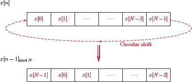
For the time reversal operation consider the following steps:
- Obtain periodic extension from x[n] using Eqn. (5.246).
- Apply the time reversal operation to to obtain .
- Obtain an length-N signal g[n] by extracting the main period of .
The resulting signal g[n] is a circularly time reversed version of x[n], that is
The process that led to Eqn. (5.269) is illustrated in Fig. 5.51 for an example length-8 signal.

Software resources: |
See MATLAB Exercise 5.7. |
For DFT-related operations the definitions of conjugate symmetry properties also need to be adjusted so that they utilize circular time reversals. A length-8 signal x[n] is circularly conjugate symmetric if it satisfies
or circularly conjugate antisymmetric if it satisfies
A signal that satisfies neither Eqn. (5.270) nor Eqn. (5.271) can still be decomposed into two components such that one is circularly conjugate symmetric and the other is circularly conjugate antisymmetric. The conjugate symmetric component is computed as
and the conjugate antisymmetric component is computed as
respectively, so that
Software resources: |
See MATLAB Exercise 5.8. |
We are now ready to explore the properties of the DFT. All properties listed in this section assume length-N signals and transforms.
Linearity
Let x1[n] and x2[n] be two length-N signals with discrete Fourier transforms
It can be shown that
for any two arbitrary constants α1 and α2.
Linearity property is easily proven starting with the forward DFT equation in Eqn. (5.255).
Time shifting
Given a transform pair
it can be shown that
Circular shifting of the signal x[n] causes the DFT to be multiplied by a complex exponential function.
Consistency check: Let the signal be circularly shifted by exactly one period, that is, m = N. We know that
In this case the exponential function on the right side of Eqn. (5.276) would be e−j(2π/N)kN = 1, and the transform remains unchanged, as expected.
Example 5.35: Gaining insight into the time shifting property of DFT
Let a signal x[n] be given by
where a, b, c, d represent arbitrary signal amplitudes. Write X[k], the DFT of x[n], in terms of the parameters a, b, c, d. Afterwards construct the transform
and determine the signal g[n] to which it corresponds.
Solution: The DFT of x[n] is
The transform G[k] is obtained as
Realizing that e−j2πk = 1 for any integer value of k, Eqn. (5.278) can be written as
Comparing Eqn. (5.278) with Eqn. (5.277) we conclude that G[k] is the DFT of the signal
which is a circularly shifted version of x[n], that is,
Time reversal
For a transform pair
it can be shown that
Example 5.36: Gaining insight into the time reversal property of DFT
Consider again the signal x[n] used in Example 5.35:
The transform X[k] = DFT {x[n]} was derived in Eqn. (5.277). Construct the transform
and determine the signal g[n] to which it corresponds.
Solution: Writing X[k] for each value of the index k we get
The transform G[k] is a circularly time reversed version of X[k]. Its samples are
Comparing G[k] with X[k] we conclude that the expressions for G[0] through G[3] can be obtained from those for X[0] through X[3] by simply swapping the roles of the parameters b and d. Consequently the signal g[n] is
which is a circularly reversed version of x[n], that is,
Conjugation property
For a transform pair
it can be shown that
Symmetry of the DFT
If the signal x[n] is real-valued, it can be shown that its DFT is circularly conjugate symmetric. Conversely, if the signal x[n] is purely imaginary, its transform is circularly conjugate antisymmetric. When we discuss symmetry properties in the context of the DFT we will always imply circular symmetry. If the signal x[n] is conjugate symmetric, its DFT is purely real. In contrast, the DFT of a conjugate antisymmetric signal is purely imaginary.
Symmetry properties of the DFT:
Consider a length-N signal x[n] that is complex-valued. In Cartesian complex form x[n] can be written as
Let the discrete Fourier transform X[k] of the signal x[n] be written in terms of its conjugate symmetric and conjugate antisymmetric components as
The transform relationship between x[n] and X[k] is
We know from Equation (5.281) and Equation (5.282) that the DFT of a real signal must be conjugate symmetric, and the DFT of a purely imaginary signal must be conjugate antisymmetric. Therefore it follows that the following must be valid transform pairs:
A similar argument can be made by writing the signal x[n] as the sum of a conjugate symmetric signal and a conjugate antisymmetric signal
and writing the transform X[k] in Cartesian complex form
The transform relationship between the two is
which leads to the following transform pairs:
Example 5.37: Using symmetry properties of the DFT
The DFT of a length-4 signal x[n] is given by
Without computung x[n] first, determine the DFT of xr[n], the real part of x[n].
Solution: We know from the symmetry properties of the DFT that the transform of the real part of x[n] is the conjugate symmetric part of X[k]:
The complex conjugate of the time reversed transform is
The conjugate symmetric component of X[k] is
The real part of x[n] can be found as the inverse transform of XE[k]:
Example 5.38: Using symmetry properties of the DFT to increase efficiency
Consider the real-valued signals g[n] and h[n] specified as
Devise a method of obtaining the DFTs of g[h] and h[n] by computing only one 4-point DFT and utilizing symmetry properties.
Solution: Let us construct a complex signal x[n] as
The conjugate symmetric component of X[k] is
and its conjugate antisymmetric component is
Based on the symmetry properties of the DFT we have DFT {g[n]} = XE[k] and DFT {jh[n]} = XO[k]. Therefore
and
It can easily be verified that G[k] and H[k] found above are indeed the DFTs of the two signals g[n] and h[n].
Software resources:
ex_5_38.m
Software resources: |
See MATLAB Exercise 5.9. |
Frequency shifting
For a transform pair
it can be shown that
Circular convolution
Periodic convolution of two periodic signals and was defined in Section 5.2.2, Eqn. (5.47). In this section we will define circular convolution for length-N signals in the context of the discrete Fourier transform. Let x[n] and h[n] be length-N signals. Consider the following set of steps:
Obtain periodic signals and as periodic extensions of x[n] and h[n]:
Compute as the periodic convolution of and .
Let y[n] be the length-N signal that is equal to one period of :
The signal y[n] is the circular convolution of x[n] and h[n]. It can be expressed in compact form as
Example 5.39: Circular convolution of two signals
Determine the circular convolution of the length-5 signals
and
using the definition of circular convolution given by Eqn. (5.290).
Solution: Adapting Eqn. (5.290) to length-5 signals we have
Fig. 5.52 illustrates the steps involved in computing the circular convolution. The result is
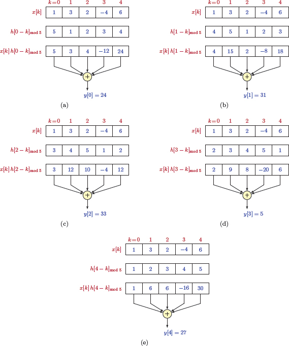
The circular convolution property of the discrete Fourier transform can be stated as follows:
Let x[n] and h[n] be two length-N signals with discrete-Fourier transforms
It can be shown that
The DFT of the circular convolution of two signals x[n] and h[n] is equal to the product of individual DFTs X[k] and H[k].
This is a very significant result in the use of the DFT for signal processing applications. The proof is straightforward using the periodic convolution property of the discrete-time Fourier series (DTFS), and will be given here.
Let and be periodic extensions of the length-N signals x[n] and h[n]. Furthermore, let and ˜ dk be the DTFS coefficients for and respectively:
The periodic convolution of and is
and the DTFS coefficients of are
We know from Eqn. (5.49) that
Recall the relationship between the DTFS and the DFT given by Eqn. (5.250). The DFTs of length-N signals x[n], h[n] and y[n] are related to the DTFS coefficients of the periodic extensions by
Using Equation (5.293), Equation (5.294) and Equation (5.295) in Eqn. (5.292) we obtain the desired result:
Example 5.40: Circular convolution through DFT
Consider again the length-5 signals x[n] and h[n] of Example 5.39. The circular convolution
was determined in Example 5.39 in the time-domain. Verify the circular convolution property of the DFT using these signals.
Solution: Table 5.5 lists the DFT for the three signals. It can easily be verified that
DFTs of the three signals in Example 5.40.
k |
X[k] |
H[k] |
Y[k] |
0 |
8.0000+j 0.0000 |
15.0000+j 0.0000 |
120.0000+j 0.0000 |
1 |
5.3992+j 0.6735 |
2.5000+j 3.4410 |
11.1803+j 20.2622 |
2 |
−6.8992-j 7.4697 |
2.5000+j 0.8123 |
−11.1803−j 24.2784 |
3 |
−6.8992+j 7.4697 |
2.5000−j 0.8123 |
−11.1803+j 24.2784 |
4 |
5.3992−j 0.6735 |
2.5000−j 3.4410 |
11.1803−j 20.2622 |
Software resources:
ex_5_40.m
If the circular convolution of two length-N signals is desired, the convolution property of the DFT provides an easy and practical method of computing it.
Obtaining circular convolution y[n] = x[n] ⊗ h[n]:
Compute the DFTs
Multiply the two DFTs to obtain Y [k].
Compute y[n] through inverse DFT:
In most applications of signal processing, however, we are interested in computing the linear convolution of two signals rather than their circular convolution. The output signal of a DTLTI system is equal to the linear convolution of its impulse response with the input signal. The ability to use the DFT as a tool for the computation of linear convolution is very important due to the availability of fast and efficient algorithms for computing the DFT. Therefore, the following two questions need to be answered:
- How is the circular convolution of two length-N signals related to their linear convolution?
- What can be done to ensure that the circular convolution result obtained using the DFT method matches the linear convolution result?
The next example will address the first question.
Example 5.41: Linear vs. circular convolution
Consider again the length-5 signals x[n] and h[n] of Example 5.39.
The circular convolution of these two signals was determined in Example 5.39 as
The linear convolution of x[n] and h[n], computed using the convolution sum
is found as
Note that in Eqn. (5.298) we have used the notation y [n] for linear convolution to differentiate it from the circular convolution result of Eqn. (5.297). The most obvious difference between the two results y[n] and y [n] is the length of each. The circular convolution result is 5 samples long, however the linear convolution result is 9 samples long. This is the first step toward explaining why the DFT method does not produce the linear convolution result. X[k] and H[k] are length-5 transforms, and the inverse DFT of their product yields a length-5 result for y[n].
How does yl [n] relate to y[n]? Imagine filling out a form that has 5 boxes for entering values, yet we have 9 values we must enter. We start from with the leftmost box and enter the first 5 of 9 values. At this point each box has a value in it, and we still have 4 more values not entered into any box. Suppose we decide to go back to the leftmost box, and start entering additional values into each box as needed. This is illustrated in Fig. 5.53 using the samples of the linear convolution result to fill the boxes.
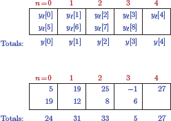
Each sample of the circular convolution result is equal to the sum of values in the corresponding box. For example, y[0] = yl [0] + yl [5] and y[1] = yl [1] + yl [6]. If a box has a single value, the circular convolution result is identical to the linear convolution result for the corresponding n. For boxes that have multiple entries, the circular convolution result is a corrupted version of the linear convolution result.
Software resources:
ex_5_41.m
Generalizing the results of Example 5.41 the circular convolution of two signals can be expressed in terms of their linear convolution as
If the circular convolution result is desired to be identical to the linear convolution result, the length of the circular convolution result must be sufficient to accommodate the number of samples expected from linear convolution. Using the analogy employed in Example 5.41, namely filling out a form with the results, there must be enough “boxes” to accommodate all samples of yl[k] without any overlaps. One method of achieving this is through zero-padding x[n] and h[n] before the computation of the DFT.
Computing linear convolution using the DFT:
Given two finite length signals with Nx and Nh samples respectively
the linear convolution yl [n] = x[n] * h[n] can be computed as follows:
Anticipating the length of the linear convolution result to be Ny = Nx + Nh − 1, extend the length of each signal to Ny through zero padding:
Compute the DFTs of the zero-padded signals xp[n] and hp[n].
Multiply the two DFTs to obtain Yp[k].
Compute yp[n] through inverse DFT:
The result yp[n] is the same as the linear convolution of the signals x[n] and y[n].
See MATLAB Exercise 5.10 and MATLAB Exercise 5.11. |
5.8.4 Using the DFT to approximate the EFS coefficients
EFS representation of a continuous-time signal xa (t) periodic with a period T0 was given in Eqn. (4.72) in Chapter 4 which is repeated below:
One method of approximating the coefficients ck on a computer is by approximating the integral in Eqn. (4.72) using the rectangular approximation method. More sophisticated methods for approximating integrals exist, and are explained in detail in a number of excellent texts on numerical analysis. The rectangular approximation method is quite simple, and will be sufficient for our purposes.
Suppose we would like to approximate the following integral:
Since integrating the function g (t) amounts to computing the area under the function, a simple approximation is
We have used the sampling interval T = T0/N and assumed that N is sufficiently large for the approximation to be a good one. The area under the function g (t) is approximated using the areas of successive rectangles formed by the samples g (nT). This is depicted graphically in Fig. 5.54.

For the purpose of approximating Eqn. (4.72) let g (t) be chosen as
so that the integral in Eqn. (4.72) is approximated as
Recalling that T0 = NT and ω0 = 2π/T0, and using the discrete-time signal x[n] = xa (nT), we have
The EFS coefficients of a periodic signal can be approximated by sampling the signal at N equally spaced time instants over one period, computing the DFT of the resulting discrete-time signal x[n], and scaling the DFT result by 1/N. Some caveats are in order:
- The number of samples over one period, N, should be sufficiently large. If we want to be more rigorous, the conditions of the Nyquist sampling theorem must be observed, and the sampling rate fs = 1/T should be at least twice the highest frequency in the periodic signal x (t).
Only the first half of the DFT values can be used as approximations for positive indexed coefficients, that is
with negative indexed coefficients obtained from the second half of the DFT by
- If the conditions of the Nyquist sampling theorem cannot be satisfied in a strict sense (such as when we try to approximate the Fourier series of a pulse train which is not limited in terms of the highest frequency it contains), only the first few terms of each set in Equation (5.305) and Equation (5.306) should be used to keep the quality of the approximation acceptable.
Software resources: |
See MATLAB Exercise 5.12 and MATLAB Exercise 5.13. |
5.8.5 Using the DFT to approximate the continuous Fourier transform
It is also possible to use the DFT for approximating the Fourier transform of a non-periodic continuous-time signal. For a signal xa (t) the Fourier transform was defined by Eqn. (4.127) in Chapter 4 which is repeated here:
Suppose xa (t) is a finite-length signal that is zero outside the interval 0 ≤ t ≤ t1. The integral in Eqn. (4.127) can be written as
The integral can be evaluated in an approximate sense using the rectangular approximation technique outlined in Eqn. (5.301) with
The function g (t) needs to be sampled at N equally spaced time instants in the interval 0 ≤ t ≤ t1, and thus NT = t1. Rectangular rule approximation to the integral in Eqn. (5.308) is
Using the discrete-time signal x[n] = xa (nT) and evaluating Eqn. (5.310) at a discrete set of frequencies
where ωs is the sampling rate in rad/s, we obtain
The Fourier transform of a continuous-time signal can be approximated by sampling the signal at N equally spaced time instants, computing the DFT of the resulting discrete-time signal x[n], and scaling the DFT result by the sampling interval T. It is also possible to obtain the approximation for Xa (ω) at a more closely spaced set of frequencies than ωk = kωs/N by zero-padding x[n] prior to computing the DFT. Let
where M is an integer. Using in Eqn. (5.311) leads to
The summation on the right side of Eqn. (5.312) is the DFT of the signal x[n] zero-padded with M additional samples.
As noted in the discussion of the previous section, the conditions of the Nyquist sampling theorem apply to this case as well. Ideally we would have liked the sampling rate ωs to be at least twice the highest frequency of the signal the transform of which is being approximated. On the other hand, it can be shown that a time-limited signal contains an infinite range of frequencies, and strict adherence to the Nyquist sampling theorem is not even possible. Approximation errors are due to the aliasing that occurs in sampling a time-limited signal. For the approximation to be acceptable, we need to ensure that the effect of aliasing is negligible.
Based on the Nyquist sampling theorem, only the first half of the DFT samples in Equation (5.311) and Equation (5.312) should be used for approximating the transform Xa (ω) at positive frequencies in the range 0 ≤ ω < ωs/2. The second half of the DFT samples represent an approximation to the transform Xa (ω) in the negative frequency range −ωs/2 ≤ ω< 0.
Software resources: |
See MATLAB Exercise 5.14. |
Interactive Demo: dft_demo.m
The demo program dft_demo.m illustrates the use of DFT for approximating the Fourier transform of a continuous-time function. It is based on Eqn. (5.311), MATLAB Exercise 5.14 and Fig. 5.57.
The continuous-time function xa (t) used in MATLAB Exercise 5.14 is graphed on the left side of the screen along with its sampled form x[n]. The parameter N represents the number of samples in the time interval 0 ≤ t ≤ 1 s, and the parameter M represents the number of padded zero-amplitude samples, paralleling the development in Equation (5.307) through Equation (5.312). Magnitude and phase of the actual spectrum Xa (f) as well as the DFT based approximation are shown on the right side.
- The case in Fig. 5.57 may be duplicated with the choices of N = 8 and M = 0. We know that NT = 1 s, so the sampling interval is T = 1/N = 0.125 s, and the sampling rate is fs = 8 Hz. The approximated samples appear from f1 = −4Hz to f2 = 3 Hz with a frequency increment of Δ f = 1 Hz.
- While keeping N unchanged, set M = 8 which causes 8 zero-amplitude samples to be appended to the right of the existing samples before the DFT computation. Now there are 16 estimated samples of the transform Xa (f) starting at f1 = −4 Hz with an increment of Δ f = 0.5s.
- Set N = 16 and M = 0. The sampling rate is fs = 16 Hz now, and therefore the estimated samples start at f1 = −8 Hz and go up to f2 = 7 Hz with an increment of Δ f = 1 Hz.
- Understanding these relationships is key to understanding effective use of the DFT as a tool for analyzing continuous-time signals.
Software resources:
dft_demo.m
5.9 Further Reading
[1] R.J. Beerends. Fourier and Laplace Transforms. Cambridge University Press, 2003.
[2] A. Boggess and F.J. Narcowich. A First Course in Wavelets with Fourier Analysis. Wiley, 2011.
[3] S.C. Chapra. Applied Numerical Methods with MATLAB for Engineers and Scientists. McGraw-Hill, 2008.
[4] S.C. Chapra and R.P. Canale. Numerical Methods for Engineers. McGraw-Hill, 2010.
[5] D.G. Manolakis and V.K. Ingle. Applied Digital Signal Processing: Theory and Practice. Cambridge University Press, 2011.
[6] A.V. Oppenheim and R.W. Schafer. Discrete-Time Signal Processing. Prentice Hall, 2010.
[7] L. Tan and J. Jiang. Digital Signal Processing: Fundamentals and Applications. Elsevier Science, 2013.
[8] J.S. Walker. Fast Fourier transforms. Studies in Advanced Mathematics. Taylor & Francis, 1996.
MATLAB Exercises
MATLAB Exercise 5.1: Developing functions to implement DTFS analysis and synthesis
In this exercise we will develop two MATLAB functions to implement DTFS analysis and synthesis equations. Function SS_DTFS (..) given below computes the DTFS coefficients for the periodic signal . The vector “x” holds one period of the signal for n = 0,...,N −1. The vector “idx” holds the values of the index k for which the DTFS coefficients are to be computed. The coefficients are returned in the vector “c”
1 function c = ss_dtfs (x, idx)
2 c = zeros (size (idx)); % Create all - zero vector.
3 N = length (x); % Period of the signal.
4 for kk = 1: length (idx),
5 k = idx (kk);
6 tmp = 0;
7 for nn = 1: length (x),
8 n = nn -1; % MATLAB indices start with 1.
9 tmp = tmp + x(nn)* exp (- j *2* pi / N* k* n);
10 end ;
11 c(kk) = tmp /N;
12 end ;
13 end
The inner loop between lines 6 and 11 implements the summation in Eqn. (5.22) for one specific value of k. The outer loop between lines 4 and 12 causes this computation to be performed for all values of k in the vector “idx”.
Function ss_invdtfs (..) implements the DTFS synthesis equation. The vector “c”holds one period of the DTFS coefficients for k = 0,...,N − 1. The vector “idx”holds the values of the index n for which the signal samples are to be computed. The synthesized signal is returned in the vector “x”
1 function x = ss_invdtfs (c, idx)
2 x = zeros (size (idx)); % Create all - zero vector.
3 N = length (c); % Period of the coefficient set.
4 for nn = 1: length (idx),
5 n = idx (nn);
6 tmp = 0;
7 for kk = 1: length (c),
8 k = kk -1; % MATLAB indices start with 1.
9 tmp = tmp + c(kk)* exp (j *2* pi/ N* k* n);
10 end ;
11 x(nn) = tmp ;
12 end ;
13 end
Note the similarity in the structures of the two functions. This is due to the similarity of DTFS analysis and synthesis equations.
The functions ss_dtfs (..) and ss_invdtfs (..) are not meant to be computationally efficient or fast. Rather, they are designed to correlate directly with DTFS analysis and synthesis equations (5.22) and (5.21) respectively. A more efficient method of obtaining the same results will be discussed later in this chapter.
Software resources:
ss_dtfs.m
ss_invdtfs.m
MATLAB Exercise 5.2: Testing DTFS functions
In this exercise we will test the two functions ss_dtfs (..) and ss_invdtfs (..) that were developed in MATLAB Exercise 5.1.
Consider the signal used in Example 5.4 and shown in Fig. 5.3. It is defined by
Its DTFS coefficients can be computed using the function ss_dtfs (..) as
>> x = [0, 1, 2, 3, 4]
>> c = ss_dtfs (x, [0:4])
The signal can be reconstructed from its DTFS coefficients using the function ss_invdtfs (..) as
>> x = ss_invdtfs (c, [-12:15])
>> stem ([-12:15], real (x))
The stem graph produced matches Fig. 5.3. The use of the function real (..) is necessary to remove very small imaginary parts due to round-off error.
Next, consider the signal of Example 5.5 which is a discrete-time pulse train. We will assume a period of 40 samples and duplicate the DTFS spectra in Fig. 5.5(a), (b), and (c). Let the signal have L = 3. Its DTFS coefficients are computed and graphed as follows:
>> xa =[ones (1, 4), zeros (1, 33), ones (1, 3)]
>> ca = ss_dtfs (xa, [0:39])
>> stem ([0:39], real (ca))
Note that one period of the signal must be specified using the index range n = 0,..., 39. The DTFS coefficients for the signal with L = 5 are computed and graphed with the following lines:
>> xb =[ones (1, 6), zeros (1, 29), ones (1, 5)]
>> cb = ss_dtfs (xb, [0:39])
>> stem ([0:39], real (cb))
Finally for with L = 7 we have
>> xc =[ones (1, 8), zeros (1, 25), ones (1, 7)]
>> cc = ss_dtfs (xc, [0:39])
>> stem ([0:39], real (cc))
Software resources:
matex_5_2a.m
matex_5_2b.m
MATLAB Exercise 5.3: Developing and testing a function to implement periodic convolution
In this exercise we will develop a MATLAB function to implement the periodic convolution operation defined by Eqn. (5.47). The function ss_pconv (..) given below computes the periodic convolution of two length-N signals and . The vector “x” holds one period of the signal for n = 0,...,N − 1. Similarly, the vector “h” holds one period of the signal for n = 0,...,N − 1. One period of the periodic convolution result is returned in vector “y”.
1 function y = ss_pconv (x, h)
2 N = length (x); % Period for all three signals.
3 y = zeros (size (x)); % Create all - zero vector.
4 for n = 0: N -1,
5 tmp = 0;
6 for k = 0: N -1,
7 tmp = tmp + ss_per (x, k)* ss_per (h, n-k);
8 end ;
9 nn = n +1;
10 y(nn) = tmp ;
11 end ;
12 end
Line 7 of the code is a direct implementation of Eqn. (5.47). It utilizes the function ss_per (..), which was developed in MATLAB Exercise 1.7 for periodically extending a discrete-time signal.
The function ss_pconv (..) can easily be tested with the signals used in Example 5.8. Recall that the two signals were
and
each with a period of N = 5. The circular convolution result is obtained as follows:
>> x = [0, 1, 2, 3, 4]
>> h = [3,3,-3,-2,-1]
>> y = ss_pconv (x, h)
Software resources:
matex_5_3.m
ss_pconv.m
MATLAB Exercise 5.4: Steady-state response of DTLTI system to sinusoidal input
Consider the DTLTI system of Example 5.29 described by the difference equation
The steady-state response of the system to the input signal
was found to be
In this exercise we will obtain the response of the system to a sinusoidal signal turned on at n = 0, that is,
by iteratively solving the difference equation, and compare it to the steady-state response found in Example 5.29. MATLAB function filter (..) will be used in iteratively solving the difference equation. The script listed below computes both responses and compares them.
1 % Script : matex_5_4.m
2 %
3 n = [-10:30];
4 ytilde = 9.9305* cos (pi * n /5 -0.3139); % Steady - state
5 x = 5* cos (pi* n /5).*(n >=0);
6 y = filter ([1, -0.2], [1, -0.9, 0.36], x); % Solve diff. eqn.
7 p1 = stem (n -0.125, ytilde, 'b'),
8 hold on
9 p2 = stem (n +0.125, y, 'r '),
10 hold off
11 axis ([-11, 31, -12, 12]);
12 xlabel ('n'),
The lines 7 and 9 of the script create two stem plots that are overlaid. In order to observe the two discrete-time signals comparatively, two different colors are used. In addition, horizontal positions of the stems are offset slightly from their integer values, to the left for and to the right for y[n]. The graph produced by the script is shown in Fig. 5.55. The steady-state response is shown in blue and the response to the sinusoidal signal turned on at n = 0 is shown in red. Notice how the two responses become the same after the transient dies out after about n = 10.
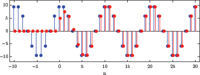
Software resources:
matex_5_4.m
MATLAB Exercise 5.5: Exploring the relationship between the DFT and the DTFT
The DFT and the DTFT of the length-10 discrete-time pulse were computed in Example 5.33. In this exercise we will duplicate the results of that example in MATLAB. The script listed below computes the 10-point DFT and graphs it on the same coordinate system with the DTFT of the signal.
1 % Script matex_5_5a.m
2 %
3 xn = ones (1, 10); % Length -10 pulse signal.
4 Xk = fft (xn); % X[k] = DFT of x[n].
5 % Create a vector ' Omega ' and compute the DTFT.
6 Omega = [-0.1:0.01:1. 1]*2 * pi + eps ;
7 XDTFT = sin (5* Omega)./ sin (0.5* Omega).* exp (- j *4.5* Omega);
8 % Compute frequencies that correspond to DFT samples.
9 k = [0:9];
10 Omega_k = 2* pi * k /10;
11 % Graph the DTFT and the DFT on the same coordinate system.
12 clf ;
13 subplot (211);
14 plot (Omega, abs (XDTFT), '-', Omega_k, abs (Xk), ' ro '), grid ;
15 axis ([-0.2* pi, 2.2* pi, -1, 11]);
16 xlabel (' Omega (rad)'),
17 ylabel (' Magnitude ')
18 subplot (212)
19 plot (Omega, angle (XDTFT), '-', Omega_k, angle (Xk), ' ro '), grid ;
20 axis ([-0.2* pi, 2.2* pi, - pi, pi]);
21 xlabel (' Omega (rad)'),
22 ylabel (' Phase (rad)'),
A slightly modified script is given below. The signal is padded with 10 additional zero-amplitude samples to extend its length to 20. This causes new transform samples to be displayed between the existing transform samples.
1 % Script matex_5_5b.m
2 %
3 xn = ones (1, 10); % Length -10 pulse signal.
4 Xk = fft (xn, 20); % X[k] = DFT of x[n] zero padded to 20.
5 % Create a vector ' Omega ' and compute the DTFT.
6 Omega = [-0.1:0.01:1. 1]* 2* pi + eps ;
7 XDTFT = sin (5* Omega)./ sin (0.5* Omega).* exp (- j *4.5* Omega);
8 % Compute frequencies that correspond to DFT samples.
9 k = [0:19];
10 Omega_k = 2* pi* k /20;
11 % Graph the DTFT and the DFT on the same coordinate system.
12 clf ;
13 subplot (211);
14 plot (Omega, abs (XDTFT), '-', Omega_k, abs (Xk), ' ro '), grid ;
15 axis ([-0.2* pi, 2.2* pi, -1, 11]);
16 xlabel (' Omega (rad)'),
17 ylabel (' Magnitude ')
18 subplot (212)
19 plot (Omega, angle (XDTFT), '-', Omega_k, angle (Xk), ' ro '), grid ;
20 axis ([-0.2* pi, 2.2* pi, - pi, pi]);
21 xlabel (' Omega (rad)'),
22 ylabel (' Phase (rad)'),
Software resources:
matex_5_5a.m
matex_5_5b.m
MATLAB Exercise 5.6: Using the DFT to approximate the DTFT
Recall from the discussion in Section 5.8.2 that zero padding a length-N signal by M additional zero-amplitude samples before the computation of the DFT results in a frequency spacing of
By choosing M large, the angular frequency spacing can be made as small as desired. This allows us to use the DFT as a tool for approximating the DTFT. If sufficient DFT samples are available, they can be graphed in the form of a continuous function of Ω to mimic the appearance of the DTFT graph. The script listed below graphs the approximate DTFT of the length-10 discrete-time pulse
The signal is padded with 490 zero-amplitude samples to extend its length to 500. The DFT result is obtained for k = 0,..., 499. The DFT sample for index k corresponds to the angular frequency Ωk = 2πk/500. The last DFT sample is at the angular frequency Ω499 = 998π/500 which is just slightly less than 2π radians.
1 % Script : matex_5_6.m
2 %
3 x = ones (1, 10); % Generate x[n].
4 Xk = fft (x, 500); % Compute 500 - point DFT.
5 k = [0:499]; % DFT indices
6 Omega_k = 2* pi * k /500; % Angular frequencies.
7 % Graph the magnitude and the phase of the DTFT.
8 clf ;
9 subplot (211);
10 plot (Omega_k, abs (Xk)); grid ;
11 title ('| X( Omega)| '),
12 xlabel (' Omega (rad)'),
13 ylabel (' Magnitude '),
14 axis ([0, 2* pi, -1, 11]);
15 subplot (212);
16 plot (Omega_k, angle (Xk)); grid ;
17 title (' angle X( Omega)'),
18 xlabel (' Omega (rad)'),
19 ylabel (' Phase (rad) '),
20 axis ([0, 2* pi, - pi, pi]);
Software resources:
matex_5_6.m
MATLAB Exercise 5.7: Developing functions for circular time shifting and time reversal
Circular versions of time shifting and time reversal operations can be implemented in MATLAB using the steps presented in Section 5.8.3. Recall that the idea behind circularly shifting a length-N signal was to first create its periodic extension with period N, then to apply time shifting to the periodic extension, and finally to extract the main period for n = 0,...,N − 1. The function ss_per (..) which was developed in MATLAB Exercise 1.7 for periodically extending a discrete-time signal will be used in constructing the functions of this exercise.
The function ss_cshift (..) listed below circularly shifts a signal by the specified number of samples. The vector “x” holds the samples of the signal x[n] for n = 0,...,N − 1. The second argument “m” is the number of samples by which the signal is to be circularly shifted. The vector “g” returned holds samples of the circularly shifted signal for n = 0,...,N − 1.
1 function g = ss_cshift (x, m)
2 N = length (x); % Length of x[n].
3 n = [0: N -1]; % Vector of indices.
4 g = ss_per (x, n - m);
5 end
The function ss_crev (..) listed below circularly reverses a signal. Again, the vector “x” holds the samples of the signal x[n] for n = 0,...,N − 1.
1 function g = ss_crev (x)
2 N = length (x); % Length of x[n].
3 n = [0: N -1]; % Vector of indices.
4 g = ss_per (x, - n);
5 end
Let us create a length-10 signal to test the functions.
>> n = [0:9];
>> x = [0, 2, 3, 4, 4.5, 3, 1, -1, 2, 1];
The signal g[n] = x[n − 3]mod 10 is obtained and graphed by typing
>> g = ss_cshift (x, 3);
>> stem (n, g);
A circular shift to the left can be obtained as well. To compute g[n] = x[n + 2]mod 10 type the following:
>> g = ss_cshift (x, -2);
A circularly time reversed version of x[n] is obtained by
>> g = ss_crev (x);
Software resources:
matex_5_7.m
ss_cshift.m
ss_crev.m
MATLAB Exercise 5.8: Computing conjugate symmetric and antisymmetric components
Any complex length-N signal or transform can be written as the sum of two components, one of which is circularly conjugate symmetric and the other circularly conjugate antisymmetric. The two components are computed using Equation (5.272) and Equation (5.273) which will be repeated here:
The terms needed in the two equations above can easily be computed using the function ss_crev (..) developed in MATLAB Exercise 5.7. Given a vector “x” that holds samples of x[n] for n = 0,...,N − 1, the signals xE[n] and xO[n] are computed as follows:
>> xE = 0.5*(x+ conj (ss_crev (x)))
>> xO = 0.5*(x - conj (ss_crev (x)))
Software resources:
matex_5_8.m
MATLAB Exercise 5.9: Using the symmetry properties of the DFT
Consider Example 5.38 where two real signals g[n] and h[n] were combined to construct a complex signal x[n]. The DFT of the complex signal was computed and separated into its circularly conjugate symmetric and antisymmetric components, and the individual transforms of g[n] and h[n] were extracted.
If the samples of the two signals are placed into MATLAB vectors “g”and “h”, the following script can be used to obtain the transforms G[k] and H[k].
1 % Script matex_5_9. m
2 %
3 x = g+j* h; % Construct complex signal.
4 Xk = fft (x); % Compute DFT.
5 % Compute the two components of the DFT.
6 XE = 0.5*(Xk+ conj (ss_crev (Xk)));
7 XO = 0.5*(Xk - conj (ss_crev (Xk)));
8 % Extract DFTs of the two signals.
9 Gk = XE;
10 Hk = -j* XO ;
11 disp (ifft (Gk)) % Should be the same as vector 'g '.
12 disp (ifft (Hk)) % Should be the same as vector 'h '.
Software resources:
matex_5_9.m
MATLAB Exercise 5.10: Circular and linear convolution using the DFT
Consider the two length-5 signals x[n] and h[n] used in Example 5.41. The script listed below computes the circular convolution of the two signals using the DFT method:
1 % Script matex_5_10a.m
2 %
3 x = [1,3,2,-4,6]; % Signal x[n]
4 h = [5, 4, 3, 2, 1]; % Signal h[n]
5 Xk = fft (x); % DFT of x[n]
6 Hk = fft (h); % DFT of y[n]
7 Yk = Xk. *Hk; % Eqn. (5.296)
8 y = ifft (Yk);
If linear convolution of the two signals is desired, the signals must be extended to at least nine samples each prior to computing the DFTs. The script given below computes the linear convolution of the two signals using the DFT method.
1 % Script : mex_5_10b.m
2 %
3 x = [1,3,2,-4,6]; % Signal x[n]
4 h = [5, 4, 3, 2, 1]; % Signal h[n]
5 xp = [x, zeros (1, 4)]; % Extend by zero padding.
6 hp = [h, zeros (1, 4)]; % Extend by zero padding.
7 Xpk = fft (xp); % DFT of xp[n]
8 Hpk = fft (hp); % DFT of hp[n]
9 Ypk = Xpk. * Hpk ; % Eqn. (5.296)
10 yp = ifft (Ypk);
The script “matex_5_10b.m” can be further simplified by using an alternative syntax for the function fft (..). The statement
>> fft (x, 9)
computes the DFT of the signal in vector “x” after internally extending the signal to nine samples by zero padding. Consider the modified script listed below:
1 % Script : matex_5_10c. m
2 %
3 x = [1,3,2,-4,6]; % Signal x[n]
4 h = [5, 4, 3, 2, 1]; % Signal h[n]
5 Xpk = fft (x, 9); % 9 - point DFT of x[n]
6 Hpk = fft (h, 9); % 9 - point DFT of h[n]
7 Ypk = Xpk. * Hpk ; % Eqn. (5.296)
8 yp = ifft (Ypk);
matex_5_10a.m
matex_5_10b.m
matex_5_10c.m
MATLAB Exercise 5.11: Developing a convolution function using the DFT
In this exercise we will develop a function for convolving two signals. Even though the built-in MATLAB function conv (..) accomplishes this task very well, it is still instructive to develop our own function that uses the DFT. As discussed in Section 5.8.3, linear convolution can be obtained through the use of the DFT as long as the length of the transform is adjusted carefully. The function ss_conv2(..) given below computes the linear convolution of two finite-length signals x[n] and h[n] the samples of which are stored in vectors “x”and “h”.
1 function y = ss_conv2 (x, h)
2 N1 = length (x); % Length of signal 'x'
3 N2 = length (h); % Length of signal 'h'
4 N = N1 + N2 -1; % Length of linear convolution result.
5 Xk = fft (x, N); % DFT of x[n] zero padded to N.
6 Hk = fft (h, N); % DFT of h[n] zero padded to N.
7 Yk = Xk. *Hk;
8 y = ifft (Yk, N);
9 end
Software resources:
ss_conv2.m
MATLAB Exercise 5.12: Exponential Fourier series approximation using the DFT
In this example, we will develop a MATLAB function to approximate the EFS coefficients of a periodic signal. The strategy used will parallel the development in Equation (5.300) through Equation (5.306). We have concluded in Section 5.8.4 that the DFT can be used for approximating the EFS coefficients through the use of Equation (5.304) and Equation (5.305) provided that the largest coefficient index k that is used in approximation is sufficiently small compared to the DFT size N.
The code for the function ss_efsapprox (..) is given below.
1 function c = ss_efsapprox(x, k)
2 Nx = length (x); % Size of vector 'x'
3 Nk = length (k); % Size of vector 'k'
4 % Create a return vector same size as 'k '.
5 c = zeros (1, Nk);
6 Xk = fft (x)/ Nx ; % Eqn. (5.304)
7 % Copy the coefficients requested.
8 for i = 1: Nk,
9 kk = k(i);
10 if (kk >= 0),
11 c(i) = Xk (kk +1);
12 else
13 c(i) = Xk (Nx +1+ kk);
14 end ;
15 end ;
16 end
The input argument x is a vector holding samples of one period of the periodic signal. The argument k is the index (or a set of indices) at which we wish to approximate the exponential Fourier series coefficients, so it can be specified as either a scalar index or a vector of index values. The return value c is either a scalar or a vector of coefficients. Its dimensions are compatible with those of k.
Suppose that 500 samples representing one period of a periodic signal have been placed into the vector x. Using the statement
>> c = ss_efsapprox(x, 2)
causes an approximate value for the coefficient c2 to be computed and returned. On the other hand, issuing the statement
>> c = ss_efsapprox(x, [-2, -1, 0, 1, 2])
results in the approximate values of coefficients {c−2,c−1,c0,c1,c2,} to be computed and returned as a vector.
To keep the function listing simple, no error checking code has been included. Therefore, it is the user’s responsibility to call the function with an appropriate set of arguments. Specifically, the index values in k must not cause an out-of-bounds error with the dimensions of the vector x. Furthermore, for good quality approximate values to be obtained, indices used should satisfy |k| << N.
Software resources:
ss_efsapprox.m
MATLAB Exercise 5.13: Testing the EFS approximation function
In this exercise we will test the function ss_efsapprox (..) that was developed in MATLAB Exercise 5.12. Consider the periodic pulse train shown in Fig. 5.56.
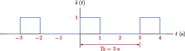
One period is defined as
We will compute 1024 samples of this signal within one period. The test code for approximating ck for k = 0,..., 10 is given below:
1 % Script : matex_5_13.m
2 %
3 t = [0:1023]/1024*3; % 1024 samples in one period.
4 x = (t (>)=1); % x(t)=1 if t (>)=1
5 % Compute and print approximate EFS coefficients for
6 % k=0,. .., 10.
7 for k = 0:10,
8 coeff = ss_efsapprox (x,k);
9 str = sprintf ('k =%3 d, magnitude =%0.5 f, phase =%0.5 f',. ..
10 k, abs (coeff), angle (coeff));
11 disp (str);
12 end ;
One point needs to be clarified: In line 3 of the code we generate a vector “t” of time samples spanning one period of T = 3 seconds. The first element of the time vector is equal to 0. We might intuitively think that the last element of this vector should be set equal to 3, the length of the period, yet it is equal to 1023(3) / (1024) which is slightly less than 3. The reason for this subtle difference becomes obvious when we look at Fig. 5.54. The width of each rectangle used in the numerical approximation of the integral is T = 3/1024. The first rectangle starts at t = 0 and extends to t = T = 3/1024. The second rectangle rectangle starts at t = T = 3/1024 and extends to t = 2T = 6/1024. Continuing to reason in this fashion, the left edge of the last rectangle of the period is at t = 1023T = 1023(3) / (1024), and the right edge of it is at t = 3. The vector “t” holds the left edge of each rectangle in the approximation, and therefore its last value is just shy of the length of the period by one rectangle width.
Actual versus approximate magnitude and phase values of exponential Fourier series coefficients of the signal are listed in Table 5.6. The same table also includes percent error calculations between actual and approximated values. Note that for index values at which the magnitude of a coefficient is zero or near-zero, phase calculations are meaningless, and percent error values are skipped.
Exact vs. approximate exponential Fourier series coefficients for the test case in MATLAB Example 5.13.
k |
Magnitude |
Phase (rad) |
||||
Actual |
Approx. |
% Error |
Actual |
Approx. |
% Error |
|
0 |
0.3333 |
0.3340 |
0.20 |
0.00 |
0.000 |
0.000 |
1 |
0.2757 |
0.2760 |
0.12 |
−1.047 |
−1.046 |
−0.098 |
2 |
0.1378 |
0.1375 |
−0.24 |
−2.094 |
−2.092 |
−0.098 |
3 |
0.0000 |
0.0007 |
0.00 |
3.142 |
0.003 |
|
4 |
0.0689 |
0.0692 |
0.47 |
−1.047 |
−1.043 |
−0.391 |
5 |
0.0551 |
0.0548 |
−0.59 |
−2.094 |
−2.089 |
−0.244 |
6 |
0.0000 |
0.0007 |
0.00 |
3.142 |
0.006 |
|
7 |
0.0394 |
0.0397 |
0.82 |
−1.047 |
−1.040 |
−0.683 |
8 |
0.0345 |
0.0341 |
−0.94 |
−2.094 |
−2.086 |
−0.390 |
9 |
0.0000 |
0.0007 |
0.00 |
3.142 |
0.009 |
|
10 |
0.0276 |
0.0279 |
1.17 |
−1.047 |
−1.037 |
−0.976 |
MATLAB Exercise 5.14: Fourier transform approximation using DFT
The continuous-time signal
has the Fourier transform (see Problem 4.33)
In this example we will develop the MATLAB code to approximate this transform using the DFT as outlined by Equation (5.311) and Equation (5.312). The MATLAB script given below computes and graphs both the actual and the approximated transforms for the signal xa (t).
- The actual transform is computed in the frequency range −10 Hz ≤ f ≤ 10 Hz.
- For the approximate solution, N = 16 samples of the signal xa (t) are taken in the time interval 0 ≤<t ≤ 1 s. This corresponds to a sampling rate of fs = 16 Hz, and to a sampling interval of T = 0.0625 s.
- Initially no zero padding is performed, therefore M = 0.
- Approximations to the continuous Fourier transform are obtained at frequencies that are spaced fs/N = 1 Hz apart.
- The DFT result has 16 samples as approximations to the continuous Fourier transform at frequencies fk = kfs/N = k Hz. Only the first 8 DFT samples are usable for positive frequencies from 0 to 7 Hz. This is due to Nyquist sampling theorem. The second half of the transform represents negative frequencies from −8Hz to −1Hz, and must be placed in front of the first half. The function fftshift (..) used in line 21 accomplishes that.
1 % Script : matex_5_14.m
2 %
3 f = [-10:0.01:10]; % Create a vector of frequencies
4 % Compute the actual transform.
5 X_actual = 0.5*(sinc (f +0.5)+ sinc (f -0.5)).* exp (-j*pi * f);
6 % Set parameters for the approximate transform
7 t1 = 1; % Upper limit of the time range
8 N = 16; % Number of samples
9 M = 0; % Number of samples for zero - padding
10 T = t1 / N; % Sampling interval
11 fs = 1/ T; % Sampling rate.
12 n = [0: N -1]; % Index n for the sampled signal x[n]
13 k = [0: N+M -1]; % Index k for the DFT X[k]
14 time = n* T; % Sampling instants
15 % Sample the signal and compute the DFT.
16 xn = sin (pi * time);
17 Xk = T* fft (xn, N+ M);
18 fk = k*fs/(N+ M);
19 % Use fftshift() function on the DFT result to bring the zero -
20 % frequency to the middle. Also adjust vector fk for it.
21 Xk = fftshift (Xk);
22 fk = fk -0.5* fs ;
23 % Graph the results.
24 clf ;
25 subplot (2, 1, 1);
26 plot (f, abs (X_actual),'-',fk, abs (Xk), 'r* '), grid ;
27 title (' Magnitude of actual and approximate transforms '),
28 xlabel ('f (Hz)'),
29 ylabel (' Magnitude '),
30 subplot (2, 1, 2);
31 plot (f, angle (X_actual), '-',fk, angle (Xk), 'r* '), grid ;
32 title (' Phase of actual and approximate transforms '),
33 xlabel ('f (Hz)'),
34 ylabel (' Phase (rad) '),
The MATLAB graph produced by the script is shown in Fig. 5.57. The zero padding parameter M can be used to control the frequency spacing. For example, setting M = 16 causes the continuous Fourier transform to be estimated at intervals of 0.5 Hz starting at −8 Hz and ending at 7.5 Hz.
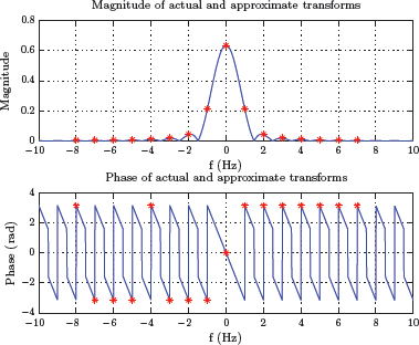
The graph obtained in MATLAB Exercise 5.14. Magnitude and phase of the actual spectrum shown are in blue, and approximated values are shown with red asterisks.
Problems
5.1. Determine the DTFS representation of the signal . Sketch the DTFS spectrum.
5.2. Determine the DTFS representation of the signal . Sketch the DTFS spectrum.
5.3. Determine the DTFS coefficients for each of the periodic signals given in Fig. P.5.3.
5.4. Consider the periodic signal of Example 5.4. Let be one sample delayed version of it, that is,
as shown in Fig. P.5.4.
- Determine the DTFS coefficients of directly from the DTFS analysis equation.
- Determine the DTFS coefficients of by applying the time shifting property to the coefficients of that were determined in Example 5.4.
5.5. Verify that the DTFS coefficients found for the signals in Problem 5.3 satisfy the conjugate symmetry properties outlined in Section 5.2.2. Since the signals are real, DTFS spectra should be conjugate symmetric.
5.6. Consider the periodic signal shown in Fig. P.5.4.
- Find even and odd components of so that
- Determine the DTFS coefficients of and . Verify the symmetry properties outlined in Section 5.2.2. The spectrum of the even component should be real, and the spectrum of the odd component should be purely imaginary.
5.7. Let and be both periodic with period N. Using the definition of periodic convolution given by Eqn. (5.49), show that the signal
is also periodic with period N.
5.8. Consider the two periodic signals shown in Fig. P.5.8.
Compute the periodic convolution
of the two signals.
Determine the DTFS coefficients of signals , and . Verify that the periodic convolution property stated by Eqn. (5.49) holds.
5.9. Repeat Problem 5.8 for the two signals shown in Fig. P.5.9.
5.10. Find the DTFT of each signal given below. For each, sketch the magnitude and the phase of the transform.
- x[n] = δ[n] + δ[n − 1]
- x[n] = δ[n] − δ[n − 1]
- x[n] = (0.7)n u[n]
- x[n] = (0.7)n cos (0.2πn) u[n]
5.11. Find the inverse DTFT of each transform specified below for −π ≤ Ω < π.
5.12. Use linearity and time shifting properties of the DTFT to find the transform of each signal given below.
- x[n] = (0.5)n u[n − 2]
- x[n] = (0.8)n (u[n] − u[n − 10])
- x[n] = (0.8)n (u[n + 5] − u[n − 5])
5.13. Use linearity and time reversal properties of the DTFT to find the transform of the signals listed below:
- x[n] = (2)n u[−n − 1]
- x[n] = (1.25)n u[−n]
- x[n] = (0.8)|n|
- x[n] = (0.8)|n| (u[n + 5] + u[n − 5])
5.14. Prove that the DTFT of a signal with odd symmetry is purely imaginary. In mathematical terms, if
5.15. Signals listed below have even symmetry. Determine the DTFT of each, and graph the magnitude of the transform.
5.16. Signals listed below have odd symmetry. For each signal determine the DTFT. Graph the magnitude and the phase of the transform.
5.17. Determine the transforms of the signals listed below using the modulation property of the DTFT. Sketch the magnitude and the phase of the transform for each.
- x[n] = (0.7)n cos (0.2πn) u[n]
- x[n] = (0.7)n sin (0.2πn) u[n]
- x[n] = cos (πn/5) (u[n] − u[n − 10])
5.18. Use the differentiation in frequency property of the DTFT to find the transforms of the signals listed below.
- x[n] = n (0.7)n u[n]
- x[n] = n (n + 1) (0.7)n u[n]
- x[n] = n (0.7)n (u[n] − u[n − 10])
5.19. Two signals x[n] and h[n] are given by
- Determine the DTFT for each signal.
- Let y[n] be the convolution of these two signals, that is, y[n] = x[n] * h[n]. Compute y[n] by direct application of the convolution sum.
Determine the DTFT of y[n] by direct application of the DTFT analysis equation. Verify that it is equal to the product of the individual transforms of x[n] and h[n]:
5.20. Determine and sketch the DTFTs of the following periodic signals.
- x[n] = ej0.3πn
- x[n] = ej0.2πn + 3ej0.4πn
- x[n] = cos (πn/5)
- x[n] = 2 cos (πn/5) + 3 cos (2πn/5)
5.21. Determine and sketch the power spectral density for each signal shown in Fig. P.5.3.
5.22. Consider the periodic signal
Recall that the DTFS representation of this signal was found in Example 5.5.
- Find the power spectral density Sx (Ω).
- Let N = 40 and L = 3. Determine what percentage of signal power is preserved if only three harmonics are kept and the others are discarded.
- Repeat part (b) with N = 40 and L = 6.
5.23. A DTLTI system is characterized by the difference equation
Determine the steady-state response of the system to the following input signals:
- x[n] = ej0.2πn
- x[n] = cos (0.2πn)
- x[n] = 2 sin (0.3πn)
- x[n] = 3 cos (0.1πn) − 5 sin (0.2πn)
Hint: First find the system function H (Ω).
5.24. Determine the steady-state response of a length-4 moving average filter to the following signals.
- x[n] = ej0.2πn
- x[n] = cos (0.2πn)
- x[n] = 2 sin (0.3πn)
- x[n] = 3 cos (0.1πn) − 5sin (0.2πn)
5.25. A DTLTI system is characterized by the difference equation
Using the technique outlined in Section 5.6.3 find the steady-state response of the system to each of the periodic signals shown in Fig. P.5.3.
5.27. Compute the DFTs of the signals given below. Simplify the results and show that each transform is purely real.
5.28. It is possible to express the forward DFT in matrix form using the compact form of the DFT definition given by Eqn. (5.253). Given the signal x[n]; n = 0,...,N − 1 and its DFT X[k]; k = 0,...,N − 1, let the vectors x and X be defined as
Show that the discrete Fourier transform can be computed as
Construct the N × N coefficient matrix W.
5.29. For each finite-length signal listed below, find the specified circularly shifted version.
5.30. Refer to Problem 5.29. Find the circularly conjugate symmetric and antisymmetric components xE[n] and xO[n] for each signal listed.
5.31. Consider the finite-length signal
- Compute the 5-point DFT X[k] for k = 0,..., 4.
- Multiply the DFT found in part (a) with e−j2πk/5 to obtain the product
- Compute the signal r[n] as the inverse DFT of R[k] and compare it to the original signal x[n].
- Repeat parts (b) and (c) with
- Provide justification for the answers found using the properties of the DFT.
5.32. Consider the finite-length signal
- Compute the 5-point DFT X[k] for k = 0,..., 4.
- Reverse the DFT found in part (a) to obtain a new transform R[k] as
- Compute the signal r[n] as the inverse DFT of R[k] and compare it to the original signal x[n]. Justify the answer found using the properties of the DFT.
5.33. The DFT of a length-6 signal x[n] is given by
Without computing x[n] first, determine
- The DFT of xr[n], the real part of x[n]
- The DFT of xi[n], the imaginary part of x[n]
5.34. Two signals x[n] and h[n] are given by
- Compute the circular convolution y[n] = x[n] ⊗ h[n] through direct application of the circular convolution sum.
- Compute the 5-point transforms X[k] and H[k].
- Compute Y [k] = X[k] H[k], and the obtain y[n] as the inverse DFT of Y [k]. Verify that the same result is obtained as in part (a).
5.35. Refer to the signals x[n] and h[n] in Problem 5.34. Let X[k] and H[k] represent 7-point DFTs of these signals, and let Y [k] be their product, that is, Y [k] = X[k] H[k] for k = 0,..., 6. The signal y[n] is the inverse DFT of Y [k]. Determine y[n] without actually computing any DFTs.
-
The DFT of a length-N signal is equal to its DTFT sampled at N equally spaced angular frequencies. In this problem we will explore the possibility of sampling a DTFT at fewer than N frequency values. Let X (Ω) be the DTFT of the length-12 signal
Obtain S[k] by sampling the transform X (Ω) at 10 equally spaced frequencies, that is,
Determine s[n], the inverse DFT of S[k].
Consider the general case where x[n] may be an infinitely long signal, and its DTFT is
S[k] is obtained by sampling X (Ω) at N equally spaced angular frequencies:
s[n] is the length-N inverse DFT of S[k]. Show that s[n] is related to x[n] by
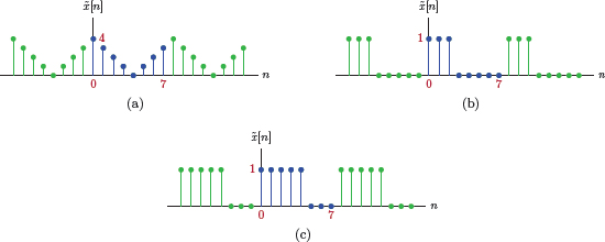


MATLAB Problems
5.37. Consider the periodic signals and shown in Fig. P.5.37.
Write a MATLAB script to do the following:
- Compute the DTFS coefficients of each signal using the function ss_dtfs (..) developed in MATLAB Exercise 5.1.
- Compute the DTFS coefficients of by multiplying the DTFS coefficients of with the proper exponential sequence as dictated by the time shifting property.
- Compare the results found in parts (a) and (b).
5.38. Consider again the periodic signals used in Problem 5.37 and shown in Fig. P.5.37. Both signals are real-valued. Consequently, their DTFS coefficients must satisfy the conjugate symmetry property as stated by Eqn. (5.35). Verify this with the values obtained in Problem 5.37.
5.39. Refer to the periodic pulse train used in Example 5.5. Write a MATLAB script to compute and graph its DTFS spectrum. Use the script to obtain graphs for the following parameter configurations:
- N = 30 , L = 5
- N = 30 , L = 8
- N = 40 , L = 10
- N = 40 , L = 15
5.40. Use the MATLAB script developed in Problem 5.39 to produce graphs that duplicate the three cases shown in Fig. 5.17 parts (a), (b) and (c).
5.41. Refer to Problem 5.22.
- Let N = 40 and L = 3. Develop a script to compute and graph a finite-harmonic approximation to x[n] using three harmonics.
- Repeat part (a) using a signal with N = 40 and L = 6.
5.42. Refer to Problem 5.24. Write a script to compute the response of the length-4 moving average filter to each of the the signals specified in the problem. Use the function ss_movavg4(..) that was developed in MATLAB Exercise 3.1 in Chapter 3. For each input signal compute the response for n = 0,..., 49. Compare the steady-state part of the response (in this case it will be after the first three samples) to the theoretical result obtained in Problem 5.24.
5.43. Refer to Problem 5.25.
- Develop a script to iteratively solve the difference equation given. The system should be assumed initially relaxed, that is, y[−1] = y[−2] = 0.
- Find the response of the system to each of the input signals in Fig. P.5.3 for n = 0,..., 49.
- In each of the responses, disregard the samples for n = 0,..., 24, and compare samples n = 25,..., 49 to the theoretical steady-state response computed in Problem 5.25.
Hint: You may wish to use the function ss_per (..) that was developed in MATLAB Exercise 1.7 for creating the periodic signals needed.
5.44. Refer to Problem 5.28 in which the matrix form of the forward DFT equation was explored.
Develop a MATLAB function ss_dftmat (..) to construct the coefficient matrix W needed in computing the DFT. Its syntax should be
W = ss_dftmat (N)where N is the size of the DFT to be computed.
Use the function ss_dftmat (..) to compute the 10-point DFT of the discrete-time pulse signal
using the matrix method. Compare the result to that obtained in Example 5.33.
- Use the function ss_dftmat (..) to compute the 20-point DFT of the discrete-time pulse signal through zero padding the vectorx. Compare the result to that obtained in Example 5.34.
5.45. Write a script to approximate the EFS coefficients of the half-wave rectified sinusoidal signal shown in Fig. P.5.45.
You may wish to use the function ss_efsapprox (..) developed in MATLAB Exercise 5.12. Sample the signal with a step size of T = 0.01 s to obtain 100 samples in one period. Obtain approximate values for the coefficients ck for k = −15,..., 15 and compare to the correct values obtained in Chapter 4, Example 4.10.
5.46. Refer to Problem 5.36 in which the issue of sampling a DTFT was explored. Develop a MATLAB script to perform the following steps:
Define an anonymous function to return the DTFT X (Ω) of the signal
Obtain S[k] by sampling the transform X (Ω) at 10 equally spaced frequencies, that is,
Compute s[n] = DFT−1 {S[k]}, and create a stem plot.
Repeat part (b) by evaluating the DTFT at 8 equally-spaced angular frequencies
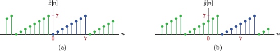
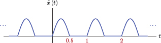
MATLAB Projects
5.47. This problem is about increasing the efficiency of DFT computation by recognizing the symmetry properties of the DFT and using them to our advantage. Recall from the symmetry properties discussed in Section 5.8.3 that for a signal expressed in Cartesian complex form
and its transform expressed using circularly conjugate symmetric and antisymmetric components as
the following relationships exist:
Develop a MATLAB script to compute the DFTs of two real-valued length-N signals r[n] and s[n] with one call to the function fft (..) using the following approach:
- Construct a complex signal x[n] = r[n] + js[n].
- Compute the DFT of the complex signal x[n] using the function fft (..).
- Find the DFTs of the signals r[n] and s[n] by splitting the transform X[k] into its two components XE[k] and XO[k] and making the necessary adjustments. You may wish to use the function ss_crev (..) developed in MATLAB Exercise 5.8.
Test your script using two 128-point signals with random amplitudes. (Use MATLAB function rand (..) to generate them.) Compare the transforms for R[k] and S[k] to results obtained by direct application of the function fft (..) to signals r[n] and s[n].
5.48. One of the popular uses of the DFT is for analyzing the frequency spectrum of a continuous-time signal that has been sampled. The theory of sampling is covered in detail in Chapter 6. In this problem we will focus on computing and graphing the approximate spectrum of a recorded audio signal using the technique discussed in Section 5.8.5.
Provided that a computer with a microphone and a sound processor is available, the following MATLAB code allows 3 seconds of audio signal to be recorded, and a vector “x” to be created with the recording:
hRec = audiorecorder;disp (' Press a key to start recording '), pause ;recordblocking (hRec, 3);disp (' Finished recording '), x = getaudiodata(hRec);By default the analog signal xa (t) captured by the microphone and the sound device is sampled at the rate of 8000 times per second, corresponding to T = 125 s. For a 3-second recording the vector “x” contains 24000 samples that represent
Develop a MATLAB script to perform the following steps to display the approximate spectrum of a speech signal xa (t):
Extract 1024 samples of the vector x[n] into a new vector.
We skip the first 8000 samples so that we do not get a blank period before the person begins to speak.
- Compute the DFT R[k] of the signal r[n]. Scale it as outlined in Section 5.8.5 so that it can be used for approximating the continuous Fourier transform of xa (t). Also create an approximate vector “f” of frequencies in Hz for use in graphing the approximate spectrum Xa (f).
- Compute and graph the decibel (dB) magnitude of the approximate spectrum as a function of frequency.
- Record your own voice and use it to test the script.