
z-Transform for Discrete-Time Signals and Systems
Chapter Objectives
- Learn the z-transform as a more generalized version of the discrete-time Fourier transform (DTFT) studied in Chapter 5.
- Understand the convergence characteristics of the z-transform and the concept of region of convergence.
- Explore the properties of the z-transform.
- Understand the use of the z-transform for modeling DTLTI systems. Learn the z-domain system function and its use for solving signal-system interaction problems.
- Learn techniques for obtaining block diagrams for DTLTI systems based on the z-domain system function.
- Learn the use of the unilateral z-transform for solving difference equations with specified initial conditions.
8.1 Introduction
In this chapter we will consider the z-transform which, for discrete-time signals, plays the same role that the Laplace transform plays for continuous-time signals. In the process, we will observe that the development of the z-transform techniques for discrete-time signals and systems parallels the development of the Laplace transform in Chapter 7.
It was established in Chapter 7 that the Laplace transform is an extension of the Fourier transform for continuous-time signals such that the latter can be thought of as a special case, or a limited view, of the former. The relationship between the z-transform and the DTFT is similar. In Chapter 5 we have discussed the use of the DTFT for analyzing discrete-time signals. The use of the DTFT was adapted to the analysis of DTLTI systems through the concept of the system function. The z-transform is an extension of the DTFT that can be used for the same purposes.
Consider, for example, a discrete-time ramp signal x [n] = nu [n]. Its DTFT does not exist since the signal is not absolute summable. We will, however, be able to use z-transform techniques for analyzing the ramp signal. Similarly, the DTFT-based system function is only usable for stable systems since the impulse response of a system must be absolute summable for its DTFT-based system function to exist. The z-transform, on the other hand, can be used with systems that are unstable as well. The DTFT may or may not exist for a particular signal or system while the z-transform will generally exist subject to some constraints.
We will see that the DTFT is a restricted cross-section of the much more general z-transform. The DTFT of a signal, if it exists, can be obtained from its z-transform while the reverse is not generally true. In addition to analysis of signals and systems, implementation structures for discrete-time systems can be developed using z-transform based techniques. Using the unilateral variant of the z-transform we will be able to solve difference equations with non-zero initial conditions.
We begin our discussion with the basic definition of the z-transform and its application to some simple signals. In the process, the significance of the issue of convergence of the transform is highlighted. In Section 8.2 the convergence properties of the z-transform, and specifically the region of convergence concept, are studied. Section 8.3 covers the fundamental properties of the transform that are useful in computing the transforms of signals with more complicated definitions. Proofs of the significant properties of the z-transform are presented to provide further insight and experience on working with transforms. Methods for computing the inverse z-transform are discussed in Section 8.4. Application of the z-transform to the analysis of linear and time-invariant systems is the subject of Section 8.5 where the z-domain system function concept is introduced. Derivation of implementation structures for discrete-time systems based on z-domain system functions is covered in Section 8.6. In Section 8.7 we discuss the unilateral variant of the z-transform that is useful in solving difference equations with specified initial conditions.
The z-transform of a discrete-time signal x[n] is defined as
where z, the independent variable of the transform, is a complex variable.
If we were to expand the summation in Eqn. (8.1) we would get an expression in the form
which suggests that the transform is a polynomial that contains terms with both positive and negative powers of z. Since the independent variable z is complex, the resulting transform X (z) is also complex-valued in general. Notationally, the transform relationship of Eqn. (8.1) can be expressed in the compact form
which is read “X(z) is the z-transform of x[n]”. An alternative way to express the same relationship is through the use of the notation
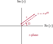
The derivation of the relationship between the z-transform and the DTFT is straightforward. Let the complex variable z be expressed in polar form as
Since z is a complex variable, we will represent it with a point in the complex z-plane as shown in Fig. 8.1. The parameter r indicates the distance of the point z from the origin. The parameter Ω is the angle, in radians, of the line drawn from the origin to the point z, measured counter-clockwise starting from the positive real axis.
Obviously, any point in the complex z-plane can be expressed by properly choosing the parameters r and Ω. Substituting Eqn. (8.5) into the z-transform definition in Eqn. (8.1) we have
The result is a function of parameters r and Ω as well as the signal x[n]. We observe from Eqn. (8.6) that X (r, Ω) represents the DTFT of the signal x[n] multiplied by an exponential signal r−n:
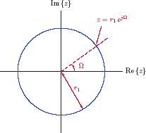
If we choose a fixed value of r = r1 in Eqn. (8.5) and allow the angle Ω to vary from 0 to 2π radians, the resulting trajectory of the complex variable z in the z-plane would be a circle with its center at the origin and with its radius equal to r1 as shown in Fig. 8.2.
This allows us to make an important observation:
Consider a circle in the z-plane with radius equal to r = r1 and center at the origin. The z-transform evaluated on this circle starting at angle Ω = 0 and ending at angle Ω = 2π is the same as the DTFT of the signal .
If the parameter r is chosen to be equal to unity, then we have z = ejΩ and
This is a significant observation. The z-transform of a signal x[n] evaluated for z = ejΩ produces the same result as the DTFT of the signal. The trajectory defined by z = ejΩ in the z-plane is a circle with unit radius, centered at the origin. This circle is referred to as the unit circle of the z-plane. Thus we can state an important conclusion:
The DTFT of a signal x[n] is equal to its z-transform evaluated at each point on the unit circle of the z-plane described by the trajectory z = ejΩ.
An easy way to visualize the relationship between the z-transform and the DTFT is the following: Imagine that the unit circle of the z-plane is made of a piece of string. Suppose the z-transform is computed at every point on the string. Let each point on the string be identified by the angle Ω so that the range −π ≤ Ω < π covers the entire piece. If we now remove the piece of string from the z-plane and straighten it up, it becomes the Ω axis for the DTFT. The values of the z-transform computed at points on the string would be the values of one period of the DTFT.
Next we would like to develop a graphical representation of the z-transform in order to illustrate its relationship with the DTFT. Suppose the z-transform of some signal x[n] is given by
In later sections of this chapter we will study techniques for computing the z-transform of a signal. At this point, however, our interest is in the graphical representation of the z-transform, the DTFT, and the relationship between them. Using the substitution z = r ejΩ, the transform in Eqn. (8.9) becomes
Using Eqn. (8.10) the transform at a particular point in the z-plane can be computed using r, its distance from the origin, and Ω, the angle it makes with the positive real axis. We would like to graph this transform; however, there are two issues that must first be addressed:
The z-transform is complex-valued. We must graph it either through its polar representation (magnitude and phase graphed separately) or its Cartesian representation (real and imaginary parts graphed separately). In this case we will choose to graph only its magnitude |X (z)| as a three-dimensional surface. The magnitude of the transform can be computed by
where X* (r, Ω) is the complex conjugate of the transform X (r, Ω), and is computed as
- Depending on the signal x[n], the transform expression given by Eqn. (8.9) is valid either for r < 0.95 only, or for r > 0.95 only. This notion will elaborated upon when we discuss the “region of convergence” concept later in this chapter. In graphically illustrating the relationship between the z-transform and the DTFT at this point, we will assume that the sample transform in Eqn. (8.9) is valid for r > 0.95. The three-dimensional magnitude surface will be graphed for all values of r; however, we will keep in mind that it is only meaningful for values of r greater than 0.95.
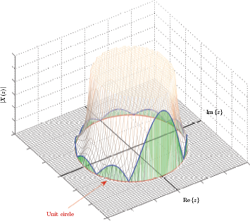
The magnitude |X (z)| is shown as a mesh in part (a) of Fig. 8.3. The unit circle is shown in the (x, y) plane. Also shown in part (a) of the figure is the set of values of |X (z)| computed at points on the unit-circle. In part (b) of Fig. 8.3 the DTFT X (Ω) of the same signal is graphed. Notice how the unit circle of the z-plane is equivalent to the horizontal axis for the DTFT.
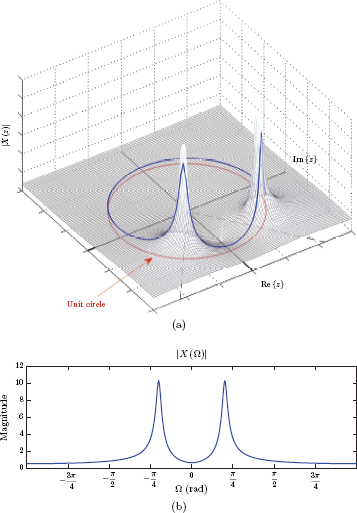
(a) The magnitude |X (z)| shown as a surface plot along with the unit circle and magnitude computed on the unit circle, (b) the magnitude of the DTFT as a function of Ω.
The z-transform defined by Eqn. (8.1) is sometimes referred to as the bilateral (two-sided) z-transform. A simplified variant of the transform termed the unilateral (one-sided) z-transform is introduced as an alternative analysis tool. The bilateral z-transform is useful for understanding signal characteristics, signal-system interaction, and fundamental characteristics of systems such as causality and stability. The unilateral z-transform is used for solving a linear constant-coefficient difference equation with specified initial conditions. We will briefly discuss the unilateral z-transform in Section 8.7, however, when we refer to z-transform without the qualifier word “bilateral” or “unilateral”, we will always imply the more general bilateral z-transform as defined in Eqn. (8.1).
Interactive Demo: zt_demo1.m
The demo program “zt_demo1.m” is based on the z-transform given by Eqn. (8.9). The magnitude of the transform in question is shown in Fig. 8.3(a). The demo program computes this magnitude and graphs it as a three-dimensional mesh. It may be rotated freely for viewing from any angle by using the rotation tool in the toolbar. The magnitude of the transform is also evaluated on a circle with radius r and graphed as a two-dimensional graph. The radius r may be varied through the use of a slider control.
Software resources:
zt_demo1.m
Software resources: |
See MATLAB Exercises 8.1 and 8.2. |
Example 8.1: A simple z-transform example
Find the z-transform of the finite-length signal
Solution: For the specified signal non-trivial samples occur for the index range n = 0,..., 4. Therefore, the z-transform is
The result is a polynomial of z−1. The samples of the signal x[n] become the coefficients of the corresponding powers of z−1. Essentially, information about time-domain sample amplitudes of the signal is contained in the coefficients of the polynomial X(z). The z-transform, therefore, is just an alternative way representing the signal x[n].
The value of the transform at a specific point in the complex plane can be evaluated from the polynomial in Eqn. (8.13). For example, if we wanted to know the value of the transform at z1 = 1 + j2 we would compute it as

The z-transform of a signal does not necessarily exist at every value of z. For example, the transform result we have found above could not be evaluated at the point z = 0 + j0 since the transform includes negative powers of z. In this case we conclude that the transform converges at all points in the complex z-plane with the exception of the origin.
Software resources:
ex_8_1.m
Example 8.2: z-Transform of a non-causal signal
Find the z-transform of the signal
Solution: This is essentially the same signal the z-transform of which we have computed in Example 8.1 with one difference: It has been advanced by two samples so it starts with index n = −2. Applying the z-transform definition given by Eqn. (8.1) we obtain
As in the previous example, the transform fails to converge to a finite value at the origin of the z-plane. In addition, the transform does not converge for infinitely large values of |z| because of the z1 and z2 terms included in X (z). It converges at every point in the z-plane with the two exceptions, namely the origin and infinity.
Example 8.3: z-Transform of the unit-impulse
Find the z-transform of the unit-impulse signal
Solution: Since the only non-trivial sample of the signal occurs at index n = 0, the z-transform is
The transform of the unit-impulse signal is constant and equal to unity. Since it does not contain any positive or negative powers of z, it converges at every point in the z-plane with no exceptions.
Example 8.4: z-Transform of a time shifted unit-impulse
Find the z-transform of the time shifted unit-impulse signal
where k ≠ 0 is a positive or negative integer.
Solution: Applying the z-transform definition we obtain
The transform converges at every point in the z-plane with one exception:
- If k > 0 then the transform does not converge at the origin z = 0 + j0.
- If k < 0 then the transform does not converge at points with infinite radius, that is, at points for which |z| → ∞.
It becomes apparent from the examples above that the z-transform must be considered in conjunction with the criteria for the convergence of the resulting polynomial X (z). The collection of all points in the z-plane for which the transform converges is called the region of convergence (ROC). We conclude from Examples 8.1 and 8.2 that the region of convergence for a finite-length signal is the entire z-plane with the possible exception of z = 0 + j0, or |z| → ∞ or both.
- The origin z = 0 + j0 is excluded from the region of convergence if any negative powers of z appear in the polynomial X (z). Negative powers of z are associated with samples of the signal x[n] with positive indices. Therefore, if the signal x[n] has any non-zero valued samples with positive indices, the z-transform does not converge at the origin of the z-plane.
- Values of z with infinite radius must be excluded from the region of convergence if the polynomial X (z) includes positive powers of z. Positive powers of z are associated with samples of x[n] that have negative indices. Therefore, if the signal x[n] has any non-zero valued samples with negative indices, that is, if the signal is non-causal, its z-transform does not converge at |z| → ∞.
For finite-length signals, the ROC can be determined based on the sample indices of the leftmost and the rightmost significant samples of the signal. If the index of the leftmost significant sample is negative, then the transform does not converge for |z| → ∞. If the index of the rightmost significant sample is positive, then the transform does not converge at the origin z = 0 + j0.
How would we determine the region of convergence for a signal that is not finite-length? Recall that in Eqn. (8.7) we have represented the z-transform of a signal x[n] as equivalent to the DTFT of the modified signal x[n]r−n. As a result, the convergence of the z-transform of x[n] can be linked to the convergence of the DTFT of the modified signal x[n]r−n. Using Dirichlet conditions discussed in Chapter 5, this requires that x[n]r−n be absolute summable, that is,
The condition stated in Eqn. (8.14) highlights the versatility of the z-transform over the DTFT. Recall that, for the DTFT of a signal x[n] to exist, the signal has to be absolute summable. Therefore, the existence of the DTFT is a binary question; the answer to it is either yes or no. In contrast, if x[n] is not absolute summable, we may still be able to find values of r for which the modified signal x[n]r−n is absolute summable. Therefore, the z-transform of the signal x[n] may exist for some values of r. The question of existence for the z-transform is not a binary one; it is a question of which values of r allow the transform to converge.
The region of convergence concept will be discussed in detail in Section 8.2. The next few examples further highlight the need for a detailed discussion of the region of convergence.
Example 8.5:z-transform of the unit-step signal
Find the z-transform of the unit-step signal
Solution: We will again apply the z-transform definition given by Eqn. (8.1).
Since u[n] = 0 for n < 0, the lower limit of the summation in Eqn. (8.15) can be changed to n = 0 without affecting the result:
Furthermore, u[n] = 1 for n ≥ 0, so dropping the u[n] term from the summation in Eqn. (8.16) has no effect either.
Eqn. (8.17) represents the sum of an infinite-length geometric series, and can be computed in closed form using the formula1 derived in Appendix C to yield
which converges only for values of z for which
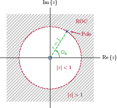
The ROC for the transform of the unit-step signal is the collection of points outside a circle with radius equal to unity. This region is shown shaded in Fig. 8.5. Note that the unit-circle itself is not part of the ROC since the transform does not converge for values of z on the circle.
![Figure showing the region of convergence for the z-transform of x[n] = u[n].](http://imgdetail.ebookreading.net/data/1/9781466598546/9781466598546__signals-and-systems__9781466598546__image__734x001.png)
Example 8.6: z-Transform of a causal exponential signal
Find the z-transform of the signal
where a is any real or complex constant.
Solution: The signal x[n] is causal since x[n] = 0 for n < 0. Applying the z-transform definition given by Eqn. (8.1) we obtain
Let us change the lower limit of the summation to n = 0 and drop the factor u[n]. Eqn. (8.18) becomes
This is the sum of an infinite-length geometric series, and can be put into a closed form as
which is valid only for values of z for which
Four possible forms of the signal x[n] are shown in Fig. 8.6a,b,c,d corresponding to possible real values of the parameter a. It should be noted that there are other possibilities; the parameter a could also have a complex value. The ROC for X (z) is the region outside a circle with radius equal to |a|. This is shown in Fig. 8.7 for |a| < 1 and |a| > 1.
![Figure showing the signal x[n] = anu[n] for (a) 0 < a < 1, (b) a > 1, (c) −1 < a < 0, and (d) a < −1.](http://imgdetail.ebookreading.net/data/1/9781466598546/9781466598546__signals-and-systems__9781466598546__image__735x001.png)
![Figure showing the region of convergence for the z-transform of x[n] = anu[n] for |a| < 1 and for |a| > 1](http://imgdetail.ebookreading.net/data/1/9781466598546/9781466598546__signals-and-systems__9781466598546__image__736x001.png)
The region of convergence for the z-transform of x[n] = an u[n] for |a| < 1 and for |a| > 1
For the case |a| < 1 the unit circle is part of the ROC whereas, for the case |a| > 1, it is not. Recall from the previous discussion that the DTFT is equal to the z-transform evaluated on the unit circle. Consequently, the DTFT of the signal exists only if the ROC includes the unit circle. We conclude that, for the DTFT of the signal x[n] to exist, we need |a| < 1. This is consistent with the existence conditions discussed in Chapter 5.
Example 8.7 z-Transform of an anti-causal exponential signal
Find the z-transform of the signal
where a is any real or complex constant.
Solution: In this case the signal x[n] is anti-causal since it is equal to zero for n ≥ 0. Applying the z-transform definition given by Eqn. (8.1) we obtain
Since
changing the upper limit of the summation to n = −1 and dropping the factor u[−n − 1] would have no effect on the result. Eqn. (8.19) simplifies to
Lower and upper summation limits are both negative. This can be fixed by employing a variable change m = −n, and the result found in Eqn. (8.20) can be written as
which has the familiar sum of geometric series, however, the lower limit of the summation is m = 1 rather than m = 0 as required for the use of the closed-form formula. Let us apply another variable change to the summation, this time in the form k = m − 1, to get the lower limit of the summation to start at k = 0:
Now the summation in Eqn. (8.21) can be put into a closed form to yield
Notice how the closed-form expression found for the signal x[n] = −an u[−n − 1] in Eqn. (8.22) is identical to the one found in Example 8.6 for a different signal, namely x[n] = an u[n]. The transform expressions are identical; however, the regions in which those expressions are valid are different. The closed-form formula found in Eqn. (8.21) is valid only for values of z for which
Four possible forms of the signal x[n] are shown in Fig. 8.8 corresponding to different ranges of the real-valued parameter a (keep in mind that a could also be complex). The ROC for the transform X (z) found in this case is the region inside a circle with radius equal to |a|. This is shown in Fig. 8.9 for |a| < 1 and |a| > 1. For the case |a| > 1 the unit circle is part of the ROC whereas, for the case |a| < 1, it is not. Thus, the DTFT of the signal x[n] exists only when |a| > 1.
![Figure showing the signal x[n] = −an u[−n − 1] for (a) 0 < a < 1, (b) a > 1, (c) −1 < a < 0, and (d) a < −1.](http://imgdetail.ebookreading.net/data/1/9781466598546/9781466598546__signals-and-systems__9781466598546__image__737x001.png)
The signal x[n] = −an u[−n − 1] for (a) 0 < a < 1, (b) a > 1, (c) −1 < a < 0, and (d) a < −1.
![Figure showing the region of convergence for the z-transform of x[n] = −an u[−n −1] for |a| < 1 and for |a| > 1.](http://imgdetail.ebookreading.net/data/1/9781466598546/9781466598546__signals-and-systems__9781466598546__image__738x001.png)
The region of convergence for the z-transform of x[n] = −an u[−n −1] for |a| < 1 and for |a| > 1.
Examples 8.6 and 8.7 demonstrate a very important concept: It is possible for two different signals to have the same transform expression for the z-transform X (z). In order for us to uniquely identify which signal among the two led to a particular transform, the region of convergence must be specified along with the transform. The following two transform pairs are fundamental in determining to which of the possible signals a given transform corresponds:
Sometimes we need to deal with the inverse problem of determining the signal x[n] that has a particular z-transform X (z). Given a transform
we need to know the region of convergence to determine if the signal x[n] is the one in Eqn. (8.23) or the one in Eqn. (8.24). This will be very important when we work with inverse z-transform in Section 8.4 later in this chapter. In order to avoid ambiguity, we will adopt the convention that the region of convergence is an integral part of the z-transform, and must be specified explicitly, or must be implied by means of another property of the underlying signal or system, every time a transform is given.
In each of the Examples 8.5, 8.6 and 8.7 we have obtained rational functions of z for the transform X (z). In the general case, a rational transform X (z) is expressed in the form
where the numerator B (z) and the denominator A (z) are polynomials of z. The parameter K is a constant gain factor. Let the numerator polynomial be written in factored form as
and let p1, p2,..., pN be the roots of the denominator polynomial so that
The transform can be written as
In Eqns. (8.26) and (8.27) the parameters M and N are the numerator order and the denominator order respectively. The larger of M and N is the order of the transform X (z). The roots of the numerator polynomial are referred to as the zeros of the transform X (z). In contrast, the roots of the denominator polynomial are the poles. The transform does not converge at a pole, therefore, the ROC cannot contain any poles. In the next section we will see that the boundaries of the ROC are determined by the poles of the transform.
Example 8.8: z-Transform of a discrete-time pulse signal
Determine the z-transform of the discrete-time pulse signal
shown in Fig. 8.10.
![Figure showing the signal x[n] for Example 8.8.](http://imgdetail.ebookreading.net/data/1/9781466598546/9781466598546__signals-and-systems__9781466598546__image__739x001.png)
Solution: The transform in question is computed as
In computing the closed-form result in Eqn. (8.29) we have used the finite-length geometric series sum formula derived in Appendix C. Since x[n] is finite-length and causal, the transform converges at every point in the z-plane except at the origin z = 0 + j0. Thus we have
Often we find it more convenient to write the transform using non-negative powers of z. Multiplying both the numerator and the denominator polynomials in Eqn. (8.29) by b zN leads to
which is in the general factored form given by Eqn. (8.28). The appearance of the closed-form result in Eqn. (8.30) may be confusing in the way it relates to the region of convergence. It seems as though X (z) might have a pole at z = 1. We need to realize, however, that the numerator polynomial is also equal to zero at z = 1:
As a result, the numerator polynomial has a (z − 1) factor that effectively cancels the pole at z = 1. We will now go through the exercise of determining the zeros and poles of the transform X (z). The roots of the numerator polynomial are found by solving the equation
In order to determine the roots of the numerator polynomial that are not immediately obvious, we will use the fact that ej2πk = 1 for all integer k, and write Eqn. (8.31) as
Taking the N-th root of both sides leads to the set of roots
The numerator polynomial of X (z) has N roots that are all on the unit circle of the z-plane. They are equally-spaced at angles that are integer multiples of 2π/N as shown in Fig. 8.11(a). Note that in the figure we have used N = 10.

Roots of the numerator polynomial zN − 1, (b) roots of the denominator polynomial zN − 1 (z − 1).
The roots of the denominator polynomial are found by solving
There are N − 1 solutions at pk = 0 and one solution at z = 1 as shown in Fig. 8.11(b).
The pole-zero diagram for the transform X (z) can now be constructed. The factors (z − 1) in numerator and denominator polynomials cancel each other, therefore there is neither a zero nor a poleat z = 1. We are left with zeros at
and a total of N − 1 poles all at
as shown in Fig. 8.12.
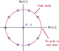
In light of what we have discovered regarding the the poles of X (z) it makes sense that the ROC is the entire z-plane with the exception of a singular point at the origin. Since all N − 1 poles of the transform are at the origin, that is the only point where the transform does not converge.
The magnitude of the z-transform computed in Eqn. (8.30) is shown in Fig. 8.13(a) as a surface graph for N = 10. Since the origin of the z-plane is excluded from the ROC, the magnitude is not computed at the origin. Also, very large magnitude values in close proximity of the origin are clipped to make the graph fit into a reasonable scale. Note how the zeros equally spaced around the unit-circle cause the magnitude surface to dip down. In addition to the surface graph, Fig. 8.13(a) also shows the unit circle of the z-plane. Magnitude values computed at points on the unit circle are marked on the surface. Fig. 8.13(b) shows the magnitude of the DTFT computed for the range of angular frequency −π ≤ Ω < π. It should be compared to the values marked on the surface graph that correspond to the magnitude of the z-transform evaluated on the unit circle.

(a) The magnitude |X (z)| shown as a surface plot along with the unit circle and magnitude computed on the unit circle, (b) the magnitude of the DTFT as a function of Ω.
To provide a slightly different perspective and to help with visualization, imagine that we take a knife and carefully cut through the surface in Fig. 8.13(a) along the perimeter of the unit-circle of the z-plane, as if the surface is a cake that we would like to fit into a cylindrical box. The profile of the cutout would match the DTFT shown in Fig. 8.13(b). This is illustrated in Fig. 8.14.
Interactive Demo: zt_demo2.m
The demo program “zt_demo2.m” is based on the z-transform of a discrete-time pulse analyzed in Example 8.8. The magnitude of the transform in question was shown in Fig. 8.13(a). The demo program computes this magnitude and graphs it as a three-dimensional mesh. It may be rotated freely for viewing from any angle by using the rotation tool in the toolbar. The magnitude of the transform is also evaluated on a circle with radius r and graphed as a two-dimensional graph. This corresponds to the DTFT of the modified signal x[n]r−n. The radius r may be varied through the use of a slider control.
Software resources:
zt_demo2.m
Example 8.9: z-Transform of complex exponential signal
Find the z-transform of the signal
The parameter Ω0 is real and positive, and is in radians.
Solution: Applying the z-transform definition directly to the signal x[n] leads to
Since x[n] is causal, the lower limit of the summation can be set to n = 0, and the u[n] term can be dropped to yield
The expression in Eqn. (8.36) is the sum of an infinite-length geometric series, and can be put into closed form as
The region of convergence is obtained from the convergence condition for the geometric series:
The transform in Eqn. (8.37) can also be written using non-negative powers of z as
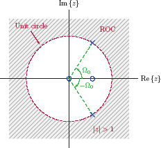
It has a zero at the origin and a pole at z = ejΩ0. The zero and the pole of the transform as well as its ROC are shown in Fig. 8.15.
Example 8.10: A more involved z-transform example
Determine the z-transform of the signal x[n] defined by
Solution: This example is somewhat tricky because of the particular way x[n] is defined. Using the definition of the z-transform we can write
The first summation in Eqn. (8.41) will be carried out for only the even values of the index n, and the second summation is for only the odd values of it. To facilitate the goal of limiting the summations to even and odd index values, we will use two variable changes: For the first summation, let n = 2m where m is the new integer index. This substitution will ensure that n is always an even value. Similarly, for the second summation, we will use the variable change n = 2m + 1 to ensure that the resulting value of n is always odd. Incorporating these variable changes into the summations, Eqn. (8.41) can be written as
or in the equivalent form
The two summations in Eqn. (8.43) can be thought of as two transforms X1 (z) and X2 (z) so that
The closed form expression for X1 (z) and its associated ROC can be obtained as
Similarly, X2 (z) is
Combining the closed form expressions for X 1 (z)and X 2 (z) as given by Eqns. (8.44) and (8.45) under a common denominator, we find the transform X (z) and its ROC as
The resulting transform has two real zeros at z = 0 and z = −0.4158 as well as a complex conjugate pair of zeros at z = 0.3746 ± j0.2451. Its poles are at and . The pole-zero diagram and the ROC for X (z) are shown in Fig. 8.16.

Example 8.11: Transform of a downsampled signal
The downsampling operation was briefly discussed in Chapter 6. Consider a signal g[n] obtained by downsampling another signal x[n] by a factor of 2:
Determine the z-transform of the downsampled signal g[n] in terms of the transform of the original signal x[n].
Solution: Using the z-transform definition, G (z) is
Let us substitute g[n] = x[2n] into Eqn. (8.47) to obtain
To resolve the summation in Eqn. (8.48) we will use the variable change m = 2n and write the summation in terms of the new index m:
Naturally, the summation should only have the terms for which m is even. This restriction on the values of the summation index makes it difficult for us to relate Eqn. (8.49) to the transform X (z) of the original signal. To overcome this hurdle we will use a simple trick. Consider a discrete-time signal w[n] with the following definition:
The transform in Eqn. (8.49) can be written as
Notice how we removed the restriction on m in Eqn. (8.50) since the factor w[m] ensures that odd-indexed terms do not contribute to the sum. One method of creating the signal w[m] is through
Substituting Eqn. (8.51) into Eqn. (8.50) we obtain
Recognizing that and , the result in Eqn. (8.52) can be rewritten as
Let the ROC for the original transform X (z) be
The ROC for and terms in Eqn. (8.53) is
and therefore the ROC for G (z) is also
Example 8.12: Transform of a downsampled signal revisited
Consider the causal exponential signal
Let a new signal g[n] be defined as g[n] = x[2n]. Find the z-transform of g[n].
Solution: The transform of the signal x[n] is
Applying the result found in Eqn. (8.53) of Example 8.11, the transform G (z) of the down-sampled signal g[n] is found as
Combining the two terms of Eqn. (8.54) under a common denominator we get
It is easy to verify the validity of the result in Eqn. (8.55) if we apply the downsampling operation in the time domain and then find the z-transform of the resulting signal g[n] directly. The time domain expression for the signal g[n] is
and its z-transform is
Software resources: |
See MATLAB Exercise 8.3. |
8.2 Characteristics of the Region of Convergence
The examples we have worked on so far made it clear that the z-transform of a discrete-time signal always needs to be considered in conjunction with its region of convergence, that is, the collection of points in the z-plane for which the transform converges. In this section we will summarize and justify the fundamental characteristics of the region of convergence.
1. The ROC is circularly shaped. It is either the inside of a circle, the outside of a circle, or between two circles as shown in Fig. 8.17.
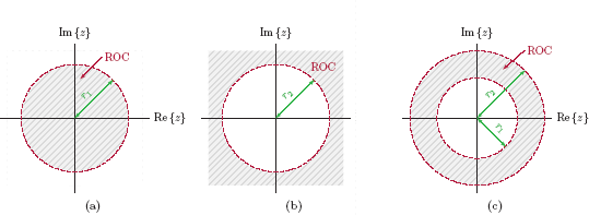
Shape of the region of convergence: (a) inside a circle, (b) outside a circle, (c) between two circles.
This property is easy to justify when we recall that, for z = r ejΩ, the values of the z-transform are identical to the values of the DTFT of the signal x[n]r−n, as derived in Eqn. (8.7). Therefore, the convergence of the z-transform for z =r ejΩ is equivalent to the convergence of the DTFT of the signal x[n]r−n which requires that
Thus, the ROC depends only on r and not on Ω, explaining the circular nature of the region. Following are the possibilities for the ROC:
2. The ROC cannot contain any poles.
By definition, poles of X (z) are values of z that make the value of the transform infinitely large. For rational z-transforms, poles are the roots of the denominator polynomial. Since the transform does not converge at a pole, the ROC must naturally exclude all poles of the transform.
3. The ROC for the z-transform of a causal signal is the outside of a circle, and is expressed as
Since a causal signal does not have any significant samples for n < 0, its z-transform can be written as
Writing z as z = rjΩ and remembering that the convergence of the z-transform is equivalent to the signal x[n]r−n being absolute summable leads to the convergence condition
which can be expressed in the equivalent form
If we can find a value of r for which Eqn. (8.58) is satisfied, then it is obvious that any larger value of r will satisfy Eqn. (8.58) as well. All we need to do is find the radius r1 of the bounding circle, and the ROC is the region outside that circle.
A special case of a causal signal is one that is both causal and finite-length. Let N1 be the largest value of the index for which the signal x[n] has a non-zero value, that is
In this case the absolute summability condition in Eqn. (8.58) can be written as
The condition in Eqn. (8.59) is satisfied for all values of r with the exception of r = 0. Our initial assessment that the ROC is the outside of a circle is still valid if we are willing to consider a circle with radius of r1 = 0, that is, one that shrinks down to a single point at the origin. The ROC for a finite-length causal signal is therefore
4. The ROC for the z-transform of an anti-causal signal is the inside of a circle, and is expressed as
The justification of this property will be similar to that of the previous one. An anti-causal signal does not have any significant samples for n ≥ 0, and its z-transform can be written as
Using z = rjΩ the condition for the convergence of the z-transform can be expressed through the equivalent condition for the absolute summability of the signal x[n]r−n as
which can be expressed in the equivalent form
Let us apply the variable change n = −m to the summation in Eqn. (8.62) to write it as
If we can find a value of r for which Eqn. (8.63) is satisfied, then it is obvious that any smaller value of r will satisfy Eqn. (8.63) as well. If r2 is the radius of the bounding circle, then the ROC is the region inside that circle.
A special case of an anti-causal signal is one that is both anti-causal and finite-length. Let −N2 be the most negative value of the index for which the signal x[n] has a non-zero value, that is
In this case the absolute summability condition in Eqn. (8.62) can be written as
The condition in Eqn. (8.64) is satisfied for all values of r that are finite; the only exception would be r → ∞. If we simply take the bounding circle to be one with infinite radius r2 = ∞ then our conclusion that the ROC is the inside of a circle is still valid, The ROC for a finite-length anti-causal signal is therefore
5. The region of convergence for the z-transform of a signal that is neither causal nor anti-causal is a ring-shaped region between two circles, and can be expressed as
Any signal x[n] can be written as the sum of a causal signal and an anti-causal signal. Let the two signals xR[n] and xL[n] be defined in terms of the signal x[n] as
and
so that xR[n] is causal, and xL[n] is anti-causal, and they add up to x[n]:
Let the z-transforms of these two signals be
The z-transform of the signal x [n] is
The ROC for X (z) is at least the overlap of the two regions, that is,
provided that r2 > r1 (otherwise there may be no overlap, and the z-transform may not exist at any point in the z-plane).
In some cases the ROC may actually be larger than the overlap in Eqn. (8.70) if the addition of the two transforms in Eqn. (8.69) results in the cancellation of a pole that sets the boundary for either XR (z) or XL (z).
As a special case, if the causal term xR[n] is of finite-length, the inner circle of the ROC may shrink down to a single point at the origin, resulting in r1 = 0. Similarly, if the anti-causal term xL[n] is of finite-length, the outer circle of the ROC may grow to have infinite radius, resulting in r2 → ∞.
Example 8.13: z-Transform of two-sided exponential signal
Find the z-transform of the signal
Solution: The specified signal exists for all values of the index n, and can be written as
or, equivalently as
We will think of x[n] as the sum of a causal signal xR[n] and an anti-causal signal xL[n] in the form
with the two components given by
When we discuss the properties of the z-transform later in Section 8.3 we will show that the z-transform is linear, and therefore, the transform of the sum of two signals is equal to the sum of their respective transforms. Therefore X (z) can be written as
The individual transforms that make up X (z) in Eqn. (8.74) can be determined by adapting the results obtained earlier in Eqns. (8.23) and (8.23) as:
The regions of convergence for XR (z) and XL (z) are shown in Fig. 8.18.
![Figure showing the region of convergence for (a) XR (z) = Ƶ{an u[n]}, (b) XL (z) = Ƶ{(1/a)n u[−n − 1]}.](http://imgdetail.ebookreading.net/data/1/9781466598546/9781466598546__signals-and-systems__9781466598546__image__752x001.png)
The region of convergence for (a) XR (z) = Ƶ{an u[n]}, (b) XL (z) = Ƶ{(1/a)n u[−n − 1]}.
The transform X (z) can now be computed as
The transform has a zero at z = 0, and poles at z = a and z = 1/a. For it to converge, both XR (z) and XL (z) must converge. Therefore, the ROC for X (z) is the overlap of the ROCs of XR (z) and XL (z) if such an over lap exists:
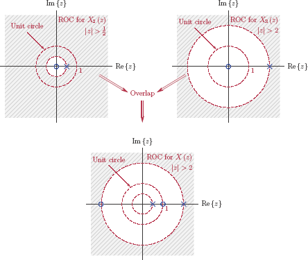
If |a| < 1, then |a| < 1/|a|, and the two regions shown in Fig. 8.18(a) and (b) do indeed overlap, creating a ring-shaped region between two circles with radii |a| and 1/|a|. This is shown in Fig. 8.19.

If |a| ≥ 1, then |a| ≥ 1/|a|, and therefore the inequality in Eqn. (8.77) cannot be satisfied for any value of z. In that case, the transform found in Eqn. (8.77) does not converge at any point in the z-plane.
8.3 Properties of the z-Transform
In this section we focus on some of the important properties of the z-transform that will help us later in using the z-transform effectively for the analysis and design of discrete-time systems. The proofs of the z-transform properties are also be given. The motivation behind discussing the proofs of various properties of the z-transform is twofold:
- The techniques used in proving various properties of the z-transform are also useful in working with z-transform problems in general.
- The proofs provide further insight into the z-transform, and allow us to later identify opportunities for the effective use of z-transform properties in solving problems.
8.3.1 Linearity
Linearity of the z-transform:
For any two signals x1[n] and x2[n] with their respective transforms
and
and any two constants α1 and α2, it can be shown that the following relationship holds:
Proof: We will prove the linearity property in a straightforward manner by using the z-transform definition given by Eqn. (8.1) with the signal α1x1[n] + α2x2[n]:
The summation in Eqn. (8.79) can be separated into two summations as
The z-transform of a weighted sum of two signals is equal to the same weighted sum of their respective transforms X1 (z) and X2 (z). The ROC for the resulting transform is at least the overlap of the two individual transforms, if such an overlap exists. The ROC may even be greater than the overlap of the two regions if the addition of the two transforms results in the cancellation of a pole that sets the boundary of one of the two regions.
The linearity property proven above for two signals can be generalized to any arbitrary number of signals. The z-transform of a weighted sum of any number of signals is equal to the same weighted sum of their respective transforms.
Example 8.14: Using the linearity property of the z-transform
Determine the z-transform of the signal
Solution: A general expression for the z-transform of the causal exponential signal was found in Example 8.6 as
Applying this result to the exponential terms in x [n] we get
and
Combining the results in Eqns. (8.81) and (8.82) using the linearity property we arrive at the desired result:
The ROC for X (z) is the overlap of the two regions in Eqns. (8.81) and (8.82), namely
The ROC for the transform X (z) is shown in Fig. 8.20 along with poles and zeros of the transform.

Example 8.15: z-Transform of a cosine signal
Find the z-transform of the signal
Solution: Using Euler’s formula for the cos (Ω0n) term, the signal x[n] can be written as
and its z-transform is
Applying the linearity property of the z-transform, Eqn. (8.85) becomes
Combining the terms of Eqn. (8.86) under a common denominator we have
Let us multiply both the numerator and the denominator by z2 to eliminate negative powers of z:
Poles of X (z) are both on the unit circle of the z-plane at z = e±jΩ0. Since x[n] is causal, the ROC is the outside of the unit circle. The unit circle itself is not included in the ROC. This is illustrated in Fig. 8.21.
Example 8.16: z-Transform of a sine signal
Find the z-transform of the signal
Solution: This problem is quite similar to that in Example 8.15. Using Euler’s formula for the signal x[n] we get
and its z-transform is
Combining the terms of Eqn. (8.90) under a common denominator we have
or, using non-negative powers of z,
The ROC of the transform is |z| > 1 as in the previous example.
8.3.2 Time shifting
Given the transform pair
the following is also a valid transform pair:
Thus, shifting the signal x[n] in the time domain by k samples corresponds to multiplication of the transform X (z) by z−k. The ability to express the z-transform of a time-shifted version of a signal in terms of the z-transform of the original signal will be very useful in working with difference equations.
Proof: The z-transform of x [n − k] is
Let us define a new variable m = n − k, and write the summation in Eqn. (8.93) in terms of this new variable:
The region of convergence for the resulting transform z−k X (z) is the same as that of X (z) with some possible exceptions:
- If time-shifting the signal for k < 0 samples (left shift) causes some negative indexed samples to appear in x [n − k], then points at |z| → ∞ need to be excluded from the ROC.
- If time-shifting the signal for k > 0 samples (right shift) causes some positive indexed samples to appear in x[n − k], then the origin z = 0 + j0 of the z-plane needs to be excluded from the ROC.
Example 8.17: z-Transform of discrete-time pulse signal revisited
The z-transform of the discrete-time pulse signal
was determined earlier in Example 8.8. Find the same transform through the use of linearity and time-shifting properties.
Solution: The signal x[n] can be expressed as the difference of a unit-step signal and a time-shifted unit-step signal, that is,
We know from the linearity property of the z-transform that
The z-transform of the unit-step function was found in Example 8.5 as
Using the time-shifting property of the z-transform, we find the transform of the shifted unit-step signal as
Adding the two transforms in Eqns. (8.98) and (8.99) yields
The result in Eqn. (8.100) can be simplified to
which matches the earlier result found in Example 8.8. Since x[n] is a finite-length causal signal, the transform converges everywhere except at the origin. Thus, the region of convergence is
This is one example of the possibility mentioned earlier regarding the region of convergence: The ROC for X (z) is larger than the overlap of the two regions given by Eqns. (8.98) and (8.99). The individual transforms Ƶ{u[n]} and Ƶ{u[n − N]} each have a pole at z = 1 causing the individual ROCs to be the outside of a circle with unit radius. When the two terms are added to construct X (z), however, the pole at z = 1 is canceled, resulting in the region of convergence for X (z) being larger than the overlap of the individual regions.
8.3.3 Time reversal
Given the transform pair
the following is also a valid transform pair:
Proof: The z-transfom of the time-reversed signal x[−n] is found by
We will employ a variable change m = −n on the summation of Eqn. (8.103) to obtain
The summation in Eqn. (8.104) starts at m = +∞ and moves toward m = −∞, adding terms from right to left. The two limits can be swapped without affecting the result since it does not matter whether we add terms from right to left or the other way around. We will also use zm = (z−1)−m to write the relationship in Eqn. (8.104) as
to prove the time-reversal property.
Since we have replaced z by z−1 in the transform, the ROC must be adjusted for this change. Let the ROC of the original transform X (z) be
The ROC for X(z−1) is
Example 8.18: z-Transform of anti-causal exponential signal revisited
The z-transform of the anti-causal exponential signal
was found in Example 8.7 as
Obtain the same result from the z-transform of the causal exponential signal using the time-reversal and time-shifting properties.
Solution: We will start with the known transform relationship and try to convert it into the relationship that we seek, applying appropriate properties of the z-transform at each step. The causal exponential signal and its z-transform are
where we have used the parameter b instead of a. Let us begin by applying the time-reversal operation to the signal on the left, and adjusting the transform on the right according to the time-reversal property of the z-transform:
The transform relationship in Eqn. (8.107) can be written in the equivalent form
We will now apply a time shift to the signal by one sample to the left through the substitution n → n + 1 which causes the transform to be multiplied by z, resulting in the relationship
Multiplying both sides of the relationship by −b leads to
Finally, choosing b = 1/a, we obtain the desired result:
8.3.4 Multiplication by an exponential signal
Given the transform pair
the following is also a valid transform pair:
Proof: The z-transform of an x[n] is
The ROC must be adjusted for the new transform variable (z/a). Let the ROC of the original transform X (z) be
The ROC for X (z/a) is
Example 8.19: Multiplication by an exponential signal
Determine the z-transform of the signal
Assume a is real.
Solution: Let the signal x1[n] be defined as
so that
The z-transform of the signal x1[n] was found in Example 8.15 to be
Multiplication of the time-domain signal by an causes the transform to be evaluated for z → z/a, resulting in the transform relationship
The transform X (z) has two poles at z = ae±jΩ0. Its ROC is
The pole-zero diagram and the ROC are shown in Fig. 8.22.

8.3.5 Differentiation in the z-domain
Given the transform pair
the following is also a valid transform pair:
Proof: Let us start with the z-transform definition
Differentiating both sides with respect to z we obtain
Since summation and differentiation are both linear operators, their order can be changed: The derivative of a sum is equal to the sum of derivatives.
Carrying out the differentiation on each term inside the summation we obtain
from which the z-transform of n x[n] can be obtained as
Thus we prove Eqn. (8.116). The ROC for the transform of n x[n] is the same as that of x[n].
Example 8.20: Using the differentiation property
Determine the z-transform of the signal
Solution: In Example 8.6 we found the z-transform of a causal exponential signal to be
Applying the differentiation property given by Eqn. (8.116) we get
and the ROC is
Example 8.21: z-Transform of a unit-ramp signal
Determine the z-transform of the unit-ramp signal
Solution: The solution is straightforward if we use the result obtained in Example 8.20. The signal n an u [n] becomes the unit-ramp signal we are considering if the parameter a is set equal to unity. Setting a = 1 in the transform found in Example 8.20 we have
with the ROC
Example 8.22: More on the use of the differentiation property
Determine the z-transform of the signal
Solution: The signal x[n] can be written as
The z-transform of the unit-ramp function was found in Example 8.21 through the use of the differentiation property as
We will now apply the differentiation property to the transform pair in Eqn. (8.124):
Finally, combining the results in Eqns. (8.124) and (8.125) we construct the z-transform of x[n] as
The transform found in Eqn. (8.126) has three poles at z = 1. Its zeros are at z = 0 and . The pole-zero diagram and the ROC are shown in Fig. 8.23.

8.3.6 Convolution property
Convolution property of the z-transform is fundamental in its application to DTLTI systems. It forms the basis of the z-domain system function concept that will be explored in detail in Section 8.5.
For any two signals x1[n] and x2[n] with their respective transforms
it can be shown that the following transform relationship holds:
Proof: We will carry out the proof by using the convolution result inside the z-transform definition. Recall that the convolution of two discrete-time signals x1[n] and x2 [n] is given by
Inserting this in to the z-transform definition we obtain
Interchanging the order of the two summations in Eqn. (8.128) leads to
Recognizing that the inner summation on the right side of Eqn. (8.129) represents the z-transform of x2[n − k] and is therefore equal to
we obtain
As before, the ROC for the resulting transform is at least the overlap of the two individual transforms, if such an overlap exists. It may be greater than the overlap of the two regions if the multiplication of the two transforms X1 (z) and X2 (z) results in the cancellation of a pole that sets a boundary for either X1 (z) or X2 (z).
Convolution property of the z-transform is very useful in the sense that it provides an alternative to actually computing the convolution of two signals in the time-domain. Instead, we can obtain x[n] = x1[n] * x2[n] using the procedure outlined below:
Finding convolution result through z-transform:
To compute x[n] = x1[n] * x2[n]:
- Find the z-transforms of the two signals.
- Multiply the two transforms to obtain X (z).
- Compute x[n] as the inverse z-transform of X (z).
Example 8.23: Using the convolution property
Consider two signals x1[n] and x2[n] given by
and
Let x[n] be the convolution of these two signals, i.e.,
Determine x[n] using z-transform techniques.
Solution: Convolution of these two signals was computed in Example 3.19 of Chapter 1 using the time-domain method. In this exercise we will use the z-transform to obtain the same result. Individual transforms of the signals x1[n] and x2[n] are
and
Applying the convolution property, the transform of x[n] can be written as the product of the two transforms:
Comparing the result obtained in Eqn. (8.132) with the definition of the z-transform we conclude that
Equivalently, the signal x[n] can be written as
The solution of the convolution problem above using z-transform techniques leads to an interesting result: Convolution operation can be used for multiplying two polynomials. Suppose we need to multiply two polynomials
and
and we have a convolution function available in software. To find the polynomial C (ν) = A (ν) B (ν), we can first create a discrete-time signal with the coefficients of each polynomial:
and
It is important to ensure that the polynomial coefficients are listed in ascending order of powers of ν in the signals xa[n] and xb[n], and any missing coefficients are accounted for in the form of zero-valued samples. If we now compute the convolution of the two signals as
the resulting signal xc[n] holds the coefficients of the product polynomial C (ν), also in ascending order of powers of the independent variable. This will be demonstrated in MATLAB Exercise 8.4.
Software resources: |
See MATLAB Exercise 8.4. |
Example 8.24: Finding the output signal of a DTLTI system using inverse z-transform
Consider a DTLTI system described by the impulse response
driven by the input signal
Compute the output signal y[n] through the use of z-transform techniques. Recall that this problem was solved in Example 3.21 of Chapter 3 using the convolution operation.
Solution: The z-transform of the impulse response is
The z-transform of the input signal x[n] is
The finite-length geometric series form of the transform X (z) will prove to be more convenient for use in this case. The z-transform of the output signal is found by multiplying the z-transforms of the input signal and the impulse response:
The output signal y[n] can now be found as the inverse z-transform of Y (z) with the use of linearity and time-shifting properties of the z-transform.
It can be shown that the result obtained in Eqn. (8.133) is identical to the one found in Example 3.21 when the two results are compared on a sample-by-sample basis.
Software resources:
ex_8_24.m
8.3.7 Initial value
Initial value property of the z-transform applies to causal signals only.
Given the transform pair
where x[n] = 0 for n < 0, it can be shown that
Proof: Consider the z-transform definition given by Eqn. (8.1) applied to a causal signal:
It is obvious from Eqn. (8.135) that, as z becomes infinitely large, all terms that contain negative powers of z tend to zero, leaving behind only x [0].
It is interesting to note that the limit in Eqn. (8.134) exists only for a causal signal, provided that x[0] is finite. Consequently, the convergence of limz→∞ [X(z)] can be used as a test of the causality of the signal. For a causal signal x[n], the ROC of the z-transform must include infinitely large values of z. If the transform X(z) is a rational function of z, the numerator order must not be greater than the denominator order.
Example 8.25: Using the initial value property
The z-transform of a causal signal x[n] is given by
Determine the initial value x[0] of the signal.
Solution: Using Eqn. (8.134) we get
The result can be easily justified by computing the inverse z-transform of X(z) using either partial fraction expansion or long division. These techniques will be explored in Section 8.4.
8.3.8 Correlation property
Cross-correlation of two discrete-time signals x[n] and y [n] is defined as
Given two signals x[n] and y [n] with their respective transforms
it can be shown that
Proof: We will first prove this property by applying the z-transform definition directly to the cross-correlation of the two signals.
By interchanging the order of the two summations in Eqn. (8.139) and rearranging the terms we get
Applying the variable change n − m =k to the inner summation in Eqn. (8.139) yields
which can be written in the equivalent form
Alternatively, we could have proven this property with less work by using other properties of the z-transform. It is obvious from the definition of the cross-correlation in Eqn. (8.137) that rxy[n] is the convolution of x[n] with y [−n], that is,
From the convolution property of the z-transform we know that the z-transform of rxy[n] must be the product of the individual transforms of x[n] and y [−n]:
In addition, we know from the time reversal property that
Therefore
The argument for the ROC of the transform uses the same reasoning we have employed earlier: The ROC for the resulting transform Rxy (z) is atleast the overlap of the two individual transforms, if such an overlap exists. It may be greater than the overlap of the two regions if the multiplication of the two transforms X(z) and Y(z−1) results in the cancellation of a pole that sets a boundary for either X(z) or Y(z−1).
As a special case of Eqn. (8.146), the transform of the autocorrelation of a signal x[n] can be found as
Example 8.26: Using the correlation property
Determine the cross-correlation of the two signals
and
using the correlation property of the z-transform.
Solution: The z-transform of x[n] is
Next we will determine the z-transform of y [n]:
Substituting z → z −1 in this last result we obtain
which is the z-transform of the time-reversed signal y [−n]. We have modified the ROC in Eqn. (8.148) to account for the fact that the transform variable z has been reciprocated. Now we obtain Rxy (z) by multiplying the two results in Eqns. (8.146) and (8.148):
The cross-correlation rxy[n] is the inverse z-transform of the result in Eqn. (8.149) which, using the time-shifting property of the z-transform, can be found as
Software resources:
ex_8_26.m
Example 8.27: Finding auto-correlation of a signal
Using the correlation property of the z-transform, determine the auto-correlation of the signal
Solution: The z-transform of the signal is
Substituting z −1 for z in Eqn. (8.152) we obtain
The z-transform of the auto-correlation rxx[n] is
provided that |a| < 1. Recall that in Example 8.13 we found the z-transform of the two-sided exponential signal to be
Comparing this earlier result to what we have in Eqn. (8.154) leads to the conclusion
8.3.9 Summation property
Given the transform pair
the following is also a valid transform pair:
Proof: Let a new signal be defined as
Using the definition of the z-transform given by Eqn. (8.1) in conjunction with w [n] we get
which would be difficult to put into a closed form directly. Instead, we will make use of the other properties of the z-transform discussed earlier, and employ a simple trick of writing w[n] as
Eqn. (8.158) provides us with a difference equation between w [n] and x[n]. Since the z-transform is linear, the transform of w [n] can be written as
and using the time-shifting property we have
which we can solve for W (z) to obtain
An alternative method of justifying the summation property is to think of w [n] as the convolution of the signal x[n] with the unit-step function. Using the convolution sum we can write
Consider the term u [n − k]:
Therefore, dropping the u [n − k] term from the summation in Eqn. (8.162) and adjusting the summation limits to compensate for it we have
Let us take the z-transform of both sides of Eqn. (8.164) using the convolution property of the z-transform:
which provides us with the alternative proof we seek.
Example 8.28: z-Transform of a unit-ramp signal revisited
The transform of the unit-ramp signal
was found in Example 8.21 through the use of the differentiation property. In this example we will use it as an opportunity to apply the summation property of the z-transform. The ramp signal x[n] can be expressed as the running sum of a time-shifted unit-step signal as
It can easily be verified that the definition in Eqn. (8.166) produces x[n]= 0 for n ≤ 0, and x[1] = 1,x [2] = 2, and so on, consistent with the ramp signal. The z-transform of the time-shifted unit-step signal is
Using the summation property we find the the transform X(z) as
which matches the answer found in Example 8.20.
8.4 Inverse z-Transform
Inverse z-transform is the problem of finding x[n] from the knowledge of X(z). Often we need to determine the signal x[n] that has a specified z-transform. There are three basic techniques for computing the inverse z-transform:
Direct evaluation of the inversion integral
Partial fraction expansion technique for a rational transform
Expansion of the rational transform into a power series through long division
We will focus our attention on the last two methods. The inversion integral method will be briefly mentioned, but will not be considered further due to its complexity. We will find that methods 2 and 3 will be sufficient for most problems encountered in the analysis of signals and linear systems.
8.4.1 Inversion integral
Let X(r, Ω) be the function obtained by evaluating the z-transform of a signal x[n] for z =re jΩ, that is, at points on a circle with radius equal to r. We have established in Section 8.1 that X(r, Ω) is the same as the DTFT of the signal x[n]r−n, that is
Consequently, the inverse DTFT equation given by Eqn. (5.70) should yield the signal x[n]r−n:
Multiplying both sides of Eqn. (8.169) with r n we obtain
Eqns. (8.168) through (8.170) provide us with a method for finding x[n] fromits z-transform:
Choose a value for r so that the circle with radius equal to r would be in the ROC of the transform X(z).
For the chosen value of the radius r, determine the function X(r, Ω) by setting z = rejΩ in the transform X(z):
Evaluate the integral
to find the signal x[n].
The three-step procedure outlined above can be reduced to a contour integral. Since z =re jΩ and r is a constant in the evaluation of the integral in Eqn. (8.172), we can write
and therefore
In the next step we will substitute Eqn. (8.174) into Eqn. (8.172), change re jΩ to z, and change X(r, Ω) to X(z) to arrive at the result
where we have used the contour integral symbol ∮ to indicate that the integral should be evaluated by traveling counter-clockwise on a closed contour in the z-plane within the ROC of the transform. The values of the transform X(z) on the closed contour are multiplied by zn−1 and integrated. Integration can start at an arbitrary point on the contour, but it must end at the same point. Note the similarity of the inversion integral to that given by Eqn. (7.93) for the computation of the inverse Laplace transform.
In general, direct evaluation of the contour integral is difficult when X(z) is a rational function of z. An indirect method of evaluating the integral in Eqn. (8.175) is to rely on the Cauchy residue theorem named after Augustin-Louis Cauchy (1789-1857). In this text we will not consider the inversion integral further for computing the inverse z-transform since more practical methods exist to accomplish the same task.
8.4.2 Partial fraction expansion
It was established in Examples 8.6 and 8.7 that the z-transform of a causal exponential signal is
and the z-transform of an anti-causal exponential signal is
The two signals in Eqns. (8.176) and (8.177) lead to the same rational function for the transform, albeit with different ROCs. These two transform pairs can be used as the basis for determining the inverse z-transform of rational functions expressed using partial fractions. Consider a transform X(z) given with its denominator factored out as
Provided that the order of the numerator polynomial B (z) is not greater than N, expanding the transform into partial fractions in the form
would allow us to use the standard forms in Eqns. (8.176) and (8.177) for finding the inverse transform of X(z). Let individual terms in the partial fraction expansion be
so that
The inverse transform is therefore computed as
where each contributing term x i[n] represents the inverse transform of the corresponding term on the right side of Eqn. (8.181), that is,
In order to find the correct terms xi[n] for Eqn. (8.182) we need to determine for each Xi (z) whether it is the transfom of a causal signal as in Eqn. (8.176) or an anti-causal signal as in Eqn. (8.177). These decisions must be made by looking at the ROC for X(z) and reasoning what the contribution from the ROC of each individual term Xi (z) must be in order to get the overlap that we have. Since each term in the partial fraction expansion has only one pole, we will adopt the following simple rules:
Determining inverse of each partial fraction:
If the ROC for X(z) is inside the circle that passes through the pole at zi, then the contribution of Xi (z) to the ROC is in the form |z| < |zi|, and therefore the term xi[n] is an anti-causal signal in the form
If the ROC for X(z) is outside the circle that passes through the pole at zi, then the contribution of Xi (z) to the ROC is in the form |z| > |zi|, and therefore the term xi[n] is a causal signal in the form
These two rules are illustrated in Fig. 8.24. The next two examples will serve to clarify the process explained above.

Determining the inverse of each term in partial fraction expansion: (a) ROC is inside the circle that passes through the pole at zi, (b) ROC is outside the circle that passes through the pole at zi.
Example 8.29: Expanding a rational z-transform into partial fractions
Express the z-transform
using partial fractions.
Solution: The first step is to divide X(z) by z to obtain
The function X(z)/z has three single poles at z = 0, ½, and 2, and can be expressed as
Multiplying both sides of Eqn. (8.187) by z allows us to express X(z) using familiar terms:
The transition from Eqn. (8.187) to Eqn. (8.188) explains the motivation for dividing X(z) by z in Eqn. (8.186) before expanding the result into partial fractions in Eqn. (8.187). Had we not divided X(z) by z in Eqn. (8.187), we would not have obtained partial fractions in the standard form z/ (z − pi)) in Eqn. (8.188).
The residues in Eqn. (8.187) can be found by using the residue formulas derived in Appendix E:
Using the residues computed, the transform X(z) is
Software resources: |
See MATLAB Exercise 8.5. |
Example 8.30: Finding the inverse z-transform using partial fractions
Consider again the transform X(z) expanded into partial fractions in Example 8.29. The region of convergence was not specified in that example, and therefore, we have only determined the partial fraction expansion for X(z).
How many possibilities are there for the ROC?
For each possible choice of ROC, determine the inverse transform.
Solution: A pole-zero diagram for X(z) is shown in Fig. 8.25. We know from previous discussion that

- There can be no poles in the ROC.
- The boundaries of ROC must be determined by poles.
We will begin by defining the three components of X(z) in the partial fraction expansion given by Eqn. (8.189). Let
and
The first component,X 1 (z), is a constant, and its ROC is always the entire z-plane. Therefore it has no effect on the overall ROC for X(z). The inverse transform of X1 (z) is
The ROC of X(z) will be determined based on the individual ROCs of the terms X2 (z) and X3 (z). The term X2 (z) has a zero at z =0, and a pole at z = ½. Its region of convergence is either the inside or the outside of the circle with a radius of ½. Similarly, the term X3 (z) has a zero at z =0, and a pole at z = 2. Its region of convergence is either the inside or the outside of the circle with a radius of 2. Applying the rules (a) and (b) mentioned above in conjunction with the pole-zero diagram shown in Fig. 8.25 we obtain the following possibilities for the ROC of X(z):
Possibility 1:
In this case both X2 (z) and X3 (z) must correspond to anti-causal signals, so that the overlap of individual ROCs yields the region chosen. Thus we need
The resulting ROC for X(z) is the overlap of the two individual ROCs, and is therefore the inside of the circle with radius ½. This is illustrated in Fig. 8.26.
The inverse transforms of X2 (z) and X3 (z) are determined using the anti-causal signal given by Eqn. (8.177):

Combining Eqns. (8.189), (8.189) and (8.190) we find the signal x[n] to be
Numerical evaluation of x [n] in Eqn. (8.191) for a few values of the index n results in
Possibility 2: ROC: |z| > 2
This ROC is only possible as the overlap of individual ROCs if both X2 (z) and X3 (z) correspond to causal signals, that is,
The resulting ROC for X (z) in this case is the overlap of the two individual ROCs which is the outside of the circle with a radius of 2. This is illustrated in Fig. 8.27.
In this case, the inverse transforms of both X2 (z) and X3 (z) are causal signals, and they are computed from Eqn. (8.176) as
Using Eqns. (8.189), (8.192) and (8.193) the inverse transform for X (z) is
In this case the first few samples of x[n] are computed as
Possibility 3:
For this ROC to be the overlap of the two individual ROCs, X2 (z) must correspond to a causal signal while X3 (z) corresponds to an anti-causal signal. We need
Thus the ROC for X2 (z) is the outside of a circle, and the ROC for X3 (z) is the inside of a circle. The overlap of the two ROCs is the region between the two circles. Fig. 8.28 illustrates this possibility.

Inverting each component accordingly, we obtain
and
Using Eqns. (8.189), (8.195) and (8.196) the inverse transform for X (z) can be constructed as
In this case the first few samples of x[n] are computed as
8.4.3 Long division
An alternative method for computing the inverse z-transform is the long division technique. Recall that the definition of the z-transform given by Eqns. (8.1) and (8.2) is essentially in the form of a power series involving powers of z and z−1. The long division idea is based on converting a rational transform X (z) back into its power series form, and associating the coefficients of the power series with the sample amplitudes of the signal x [n]. In contrast with the partial fraction expansion method discussed in the previous section, the long division method does not produce an analytical solution for the signal x [n]. Instead, it allows us to obtain the signal one sample at a time. Its main advantage over the partial fraction expansion method is that it is suitable for use on a computer.
Consider a rational transform in the general form
where the M-th order denominator polynomial B (z) is
and the N-th order numerator polynomial A (z) is
Initially we will focus on the case where the signal x [n] that led to the transform X (z) is causal. This implies the following:
- The ROC is in the form |z| > r1.
- The transform X (z) converges at |z| → ∞.
- The order of the numerator is less then or equal to the order of the denominator, that is, M ≤ N.
Dividing the numerator polynomial by the denominator polynomial, the transform X (z) can be written in the alternative form
where (bM /aN)z −(N−M) is the quotient of the division. The remainder is a polynomial in the form
Associating the expression in Eqn. (8.202) with the power series form of the z-transform we recognize that
providing us with one sample of the signal x [n]. We can now take the function
and repeat the process, obtaining
which produces another sample of the signal x [n] as
and a new remainder polynomial
The next example will illustrate this process.
Example 8.31: Using long division with right-sided signal
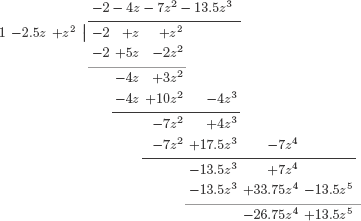
Use the long division method to determine the first few samples of the signal x [n] of Example 8.22 from its z-transform which was determined to be
Solution: By multiplying out the denominator, the transform X (z) can be written as
The numerator polynomial is
and the denominator polynomial is
Dividing the numerator polynomial by the denominator polynomial we obtain an alternative form of X (z) as
Thus we have extracted one term of the power series representation of X (z), and it indicates that x [1] = 3. Repeating the process with (z), we obtain
indicating that x [2] = 8. The results in Eqns. (8.208) and (8.209) can be combined, yielding
Thus, each iteration through the long division operation produces one more sample of the signal x [n]. We are now ready to set up the long division:

Using the quotient and the remainder of the division, the transform X (z) can be written as
Comparing the result in Eqn. (8.210) with the definition of the z-transform in Eqn. (8.1) we conclude that the signal x [n] is in the form
The sample amplitudes obtained should be in agreement with those obtained by directly evaluating the values of the signal x[n] = n(n + 2) u[n] that led to the transform in question.
In Example 8.31 the use of the long division technique produced a causal signal as the inverse transform of the specified function X (z). That was fine since the ROC specified for the transform also supported this conclusion. What if we have a transform and associated ROC that indicate an anti-causal or a non-causal signal as the inverse transform? How would we need to modify the long division technique to produce the correct result in such a case?
Consider again a rational transform X (z) with one change from Eqn. (8.198): This time we will order the terms of numerator and denominatior polynomials in ascending powers of z. The result is
If we now divide the numerator polynomial by the denominator polynomial, we can write X (z) as
The term (b0/a0) is the quotient of the division. The remainder is a polynomial in the form
Associating the expression in Eqn. (8.202) with the power series form of the z-transform we recognize that
We can now take the function
and repeat the process, obtaining
which produces another sample of the signal x [n] as
and a new remainder polynomial
The next example will illustrate the use of long division with different types of ROCs.
Example 8.32: Using long division with specified ROC
In Example 8.29 we have used the partial fraction expansion method to determine the inverse z-transform of the rational function
for all possible choices of the ROC. Verify the results of that example by determining the first few samples of the inverse z-transform through the use of the long division method for each possible choice of the ROC.
Solution: Multiplying out the factors of the numerator and the denominator of X (z) we obtain
As we have discussed in Example 8.30, there are three possible choices for the ROC:
Possibility 1:
In this case the inverse transform x [n] must be anti-causal. In order to obtain an anti-causal solution from the long division, we will rewrite X (z) with its numerator and denominator polynomials arranged in ascending powers of z :
and set up the long division:
Using the quotient and the remainder of the division, the transform X (z) can be written as
Comparing the result in Eqn. (8.220) with the z-transform definition in Eqn. (8.1) we conclude that the signal x [n] must be in the form
consistent with the answer found in Example 8.30.
Possibility 2: ROC: |z| > 2
In this case the signal x [n] is causal. To obtain a causal answer we will use the original form of X (z) in Eqn. (8.219) with numerator and denominator polynomials arranged in descending orders of z. The long division is set up as follows:
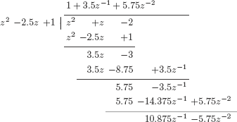
Using the results obtained so far, the transform X (z) is expressed as
The first few samples of the signal x [n] are
identical to the result that was found in Example 8.30.
Possibility 3:
In this case the inverse transform x[n] has a causal component and an anti-causal component, so it can be written in the form
Accordingly, we need to partition the transform X (z) into two parts: One that corresponds to the causal component xR[n], and one that corresponds to the anti-causal component xL[n]. Recall that in Example 8.29 the transform X (z) was expressed through partial fractions as
with
and
It is clear that X2 (z) should be included in XR (z), and X3 (z) should be included in XL (z). The constant term, X1 (z) = −2, could be included with either function; we will choose to include it with X R (z). Consequently we have
and
Let us begin with xR[n]. The long division for the causal component is set up using the numerator and the denominator of XR (z) arranged in descending powers of z:
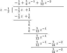
We conclude that xR[0] = −1/3, xR[1] = 5/6 and xR[2] = 5/12. Next we will set up the long division for xL[z] with numerator and denominator polynomials arranged in ascending powers of z:
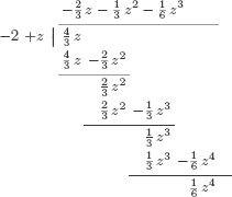
Thus, the first few samples of the anti-causal component of x[n] are xL[−1] = −2/3, xL[−2] = −1/3 and xL[−3] = −1/6. Combining the results of the two long divisions we obtain x[n] as
See MATLAB Exercise 8.6. |
8.5 Using the z-Transform with DTLTI Systems
In Chapter 3 we have demonstrated that the output signal of a DTLTI system is related to its input signal and its impulse response through the convolution sum. Specifically, if the impulse response of a DTLTI system is h [n], and if the signal x [n] is applied to the system as input, the output signal y [n] is computed as
Based on the convolution property of the z-transform introduced by Eqn. (8.127) in Section 8.3.6, the z-transform of the output signal is equal to the product of the z-transforms of the input signal and the impulse response, that is,
If the input signal x [n] and the impulse response h [n] are specified, we could find the z-transforms X (z) and H (z), multiply them to obtain Y (z), and then determine y [n] by means of inverse z-transform. This process provides us an alternative to computing the output by direct application of the convolution sum, and was demonstrated in Examples 8.23 and 8.24.
Alternatively, if the input and the output signals x [n] and y [n] are specified, their z-transforms can be computed, and then the z-transform of the impulse response can be determined from them. Solving Eqn. (8.221) for H (z) we get
The function H (z) is the z-domain system function of the system. We already know that a DTLTI system can be described fully and uniquely by means of its impulse response h [n]. Since the system function H (z) is just the z-transform of the impulse response h [n], it also represents a complete description of the DTLTI system.
8.5.1 Relating the system function to the difference equation
In Section 3.4 of Chapter 3 we have established the fact that a DTLTI system can be described by means of a constant-coefficient linear difference equation in the standard form
Therefore it must be possible to obtain the other two forms of description of the DTLTI system, namely the system function and the impulse response, from the knowledge of its difference equation. If we take the z-transform of both sides of Eqn. (8.223) the equality would still be valid:
Using the linearity property of the z-transform, Eqn. (8.224) can be written as
and using the time-shifting property of the z-transform leads to
The transforms X (z) and Y (z) do not depend on the summation index k, and can therefore be factored out of the summations in Eqn. (8.226) resulting in
Finally, the system function can be obtained from Eqn. (8.227) as
Finding the system function from the difference equation:
- Separate the terms of the difference equation so that y [n] and its time-shifted versions are on the left of the equal sign, and x [n] and its time-shifted versions are on the right of the equal sign, as in Eqn. (8.223).
- Take the z-transforms of both sides of the difference equation, and use the time-shifting property of the z-transform as in Eqn. (8.226).
- Determine the system function as the ratio of Y (z) to X (z) as in Eqn. (8.228).
- If the impulse response is needed, it can now be determined as the inverse z-transform of H (z).
At this point we will make two important observations:
- In the above development leading up to the z-domain system function we have relied on the convolution operation in Eqn. (8.221). In Eqn. (8.228) we have used the convolution property of the z-transform. We know from Chapter 3 that the convolution operation is only applicable to problems involving linear and time-invariant systems. Therefore the system function concept is meaningful only for systems that are both linear and time-invariant. This notion was introduced in earlier discussions involving system functions as well.
- Furthermore, it was justified in Section 3.4 of Chapter 3 that a constant-coefficient difference equation corresponds to a linear and time-invariant system only if all initial conditions are set to zero.
Consequently, we conclude that, in determining the system function from the difference equation, all initial conditions must be assumed to be zero.
If we need to use z-transform based techniques to solve a difference equation subject to non-zero initial conditions, we can do that through the use of the unilateral z-transform, but not through the use of the system function. The unilateral z-transform and its use for solving difference equations will be discussed in Section 8.7.
Example 8.33: Finding the system function from the difference equation
Let a DTLTI system be defined by the difference equation
Find the system function H (z) for this system.
Solution: We will assume zero initial conditions and take the z-transforms of both sides of the difference equation to get
from which the system function is obtained as
or, using non-negative powers of z
We will make another important observation based on the result obtained in Example 8.33: The characteristic equation for the system considered in Example 8.33 is
and the solutions of the characteristic equation are the modes of the system as defined in Section 3.5.1 of Chapter 3. When we find the system function H (z) from the difference equation we see that its denominator polynomial is identical to the characteristic polynomial. The roots of the denominator polynomial are the poles of the system function in the z-domain, and consequently, they are identical to the modes of the difference equation of the system.
Recall that in Section 3.5.1 we have reached some conclusions about the relationship between the modes of the difference equation and the natural response of the corresponding system. The same conclusions would apply to the poles of the system function. Specifically, if all poles pk of the system are real-valued and distinct, then the natural response is in the form
Complex poles appear in conjugate pairs provided that all coefficients of the system function are real-valued. A pair of complex conjugate poles
Finally, a pole of multiplicity m at z = p1 leads to a response in the form
Justifications for these relationships were given in Section 3.5.1 of Chapter 3 through the use of the modes of the difference equation, and will not be repeated here.
Sometimes we need to reverse the problem represented in Example 8.33 and find the difference equation from the knowledge of the system function. The next example will demonstrate this.
Example 8.34: Finding the difference equation from the system function
Find the difference equation of the DTLTI system defined by the system function
Solution: Let us first write H(z) as a rational function of z− by multiplying both its numerator and denominator with z −3:
We know that the system function is the ratio of the output transform to the input transform, that is,
so that we can write
or equivalently
8.5.2 Response of a DTLTI system to complex exponential signal
An interesting interpretation of the system function concept is obtained when one considers the response of a DTLTI system to a complex exponential signal in the form
where z0 represents a point in the z-plane within the ROC of the system function. Let h[n] be the impulse response of the DTLTI system under consideration. The output signal is determined through the use of the convolution sum
Substituting into Eqn. (8.229) and simplifying the resulting summation we obtain
In Eqn. (8.230) the summation corresponds to the system function H(z) evaluated at the point z = z0, so the response of the DTLTI system to the input signal is
We conclude that the response of a DTLTI system to the exponential signal is a scaled version of the input signal. The scale factor is the value of the system function at the point z = z0.
Example 8.35: Response of a DTLTI system to a complex exponential signal
Consider a DTLTI system with the system function
Find the response of the system to the exponential signal
Solution: The input signal is complex-valued. Using Euler’s formula we can write x [n]as
Real and imaginary parts of x [n] are shown in Fig. 8.29. The value of the system function at z = 0.9ej0.2π is
![Figure showing the signal x[n] for Example 8.35: (a) real part, (b) imaginary part.](http://imgdetail.ebookreading.net/data/1/9781466598546/9781466598546__signals-and-systems__9781466598546__image__794x001.png)
The output signal is found using Eqn. (8.231) as
or, in Cartesian form
Real and imaginary parts of the output signal y[n]are shown in Fig. 8.30.
![Figure showing the signal y [n] for Example 8.35: (a) real part, (b) imaginary part.](http://imgdetail.ebookreading.net/data/1/9781466598546/9781466598546__signals-and-systems__9781466598546__image__794x002.png)
ex_8_35a.m
ex_8_35b.m
8.5.3 Response of a DTLTI system to exponentially damped sinusoid
Next we will consider an input signal in the form of an exponentially damped sinusoid such as
In order to find the response of a DTLTI system to this signal, let us write x [n] using Euler’s formula:
Let z0 be defined as
It follows that
and Eqn. (8.233) can be written as
The response of the system is determined using the linearity of the system:
We already know that the response of the system to the term is
and its response to the term is
so that the output signal y [n] can be written as
The result obtained in Eqn. (8.238) can be further simplified. Let the value of the system function evaluated at the point z = z0 be written in polar complex form as
where H0 and Θ0 represent the magnitude and the phase of the system function at the point z = z 0 respectively:
It can be shown (see Problem 8.34 at the end of this chapter) that, for a system with a real-valued impulse response, the value of the system function at the point is the complex conjugate of its value at the point z = z0,thatis,
Using Eqns. (8.239) and (8.242) in Eqn. (8.238), the output signal y [n] becomes
Comparison of the input signal in Eqn. (8.232) and the output signal Eqn. (8.243) reveals the following:
- The amplitude of the signal is multiplied by the magnitude of the system function evaluated at the point z = r 0ejΩ.
- The phase of the cosine function is incremented by an amount equal to the phase of the system function evaluated at the point z = r0ejΩ.
Example 8.36: Response of a DTLTI system to an exponentially damped sinusoid
Consider again the system function used in Example 8.35. Determine the response of the system to the input signal
Solution: In Example 8.35 we have evaluated the system function at the point z = 0.9ej0.2π and have obtained
Using Eqn. (8.243) with H0 = 4.7526 and Θ0 = −1.7963 radians, we obtain the output signal as
The input and the output signals are shown in Fig. 8.31.
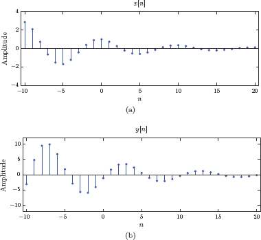
Software resources:
ex_8_36.m
8.5.4 Graphical interpretation of the pole-zero plot
It was discussed earlier in this chapter that the complex variable z can be represented as a point in the z-plane. Alternatively, a complex number can be thought of as a vector in the complex plane (see Appendix A), drawn from the origin to the point of interest. Let z = rejΩ. Fig. 8.32 illustrates the use of a vector with norm (or length) equal to r and angle equal to Ω for representing z.
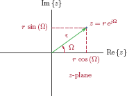
Using vector notation we will write
The norm and the angle of the vector are expressed as
Fixing Ω and changing the value of r causes the tip of the vector to move either toward or away from the origin while the direction of the vector remains unchanged. Fixing r and changing the value of Ω causes the vector to rotate while its length remains unchanged. In this case the tip of the vector stays on a circle with radius r.
Consider a fixed point z 1 in the z-plane. It will be interesting to find the vector .
Based on Eqn. (8.248) the vector can be found by adding the two vectors and using the parallelogram rule as shown in Fig. 8.33.
 .
.
Finding the vector representation for (z − z1)
Any vector is identified by two features: its norm (length) and its direction. The starting point of a vector is not important. Shifting a vector parallel to itself so that it starts at any desired point would be allowed as long as the norm and the direction of the vector are not changed. Accordingly, the vector found through the use of the parallelogram rule in Fig. 8.33 can be shifted so that it originates at the point z 1 and terminates at the point z as shown in Fig. 8.34.
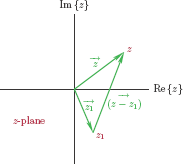 .
.The alternative representation shown in Fig. 8.34 leads us to an important conclusion:
In the z-plane, the vector is drawn with an arrow that starts at the point z1 and ends at the point z.
This conclusion will be critical in graphically interpreting the pole-zero diagram for a system function. We will begin by considering a simple DTLTI system with the impulse response
and the corresponding z-domain system function
The system has a zero at z = 0 and a pole at z = a. In vector form, the system function can be written as the ratio of two vectors
Suppose we need to evaluate the system function at a specific point z = za in the z-plane. Assuming that the point z = za is within the ROC of the system function, the vector representation of the system function at the point of interest is
with its magnitude and phase computed as
and
Example 8.37: Evaluating H(z) using vectors
Let a DTLTI system be characterized by the system function
Discuss how the system function can be graphically evaluated at the points
za = 1.5 + j1
zb = −0.5 −j1
Solution: Both points za and zb are within the ROC of the system function. For H(za) we need the vectors and shown in Fig. 8.35.

If the pole-zero diagram in Fig. 8.35 is drawn to scale, we could simply measure the lengths and the angles of the two vectors, and compute the magnitude and the phase of the system function at z = za from those measurements as
and
It can be shown that
The magnitude and the phase of the system function at za = 1. 5 + j1 are
and
To evaluate H(zb) we need the vectors and as shown in Fig. 8.36.
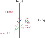
With these new vectors it can be shown that
The magnitude and the phase of the system function at za = 1.5 + j1 are
and
Vector representation of the factors that make up the system function H (z)is particularly useful for inferring the frequency response of a system from the distribution of its z-domain poles and zeros. It was shown earlier that the DTFT-based frequency response H (ω) of a DTLTI system can be obtained from the z-domain system function by evaluating H (z) at each point on the unit circle of the z-plane. Continuing with the first-order system function given by Eqn. (8.250) we obtain
In using Eqn. (8.255) we are assuming that |a| < 1 so that the ROC for the system function includes the unit circle, and therefore the frequency response H (Ω) of the system exists. Fig. 8.37 shows the two vectors
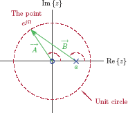
Vectors from the zero and the pole of the system function H(z) = z/(z − a) to a point on the unit circle.
and
that are needed for evaluating H (Ω). The vectors originate from the zero and the pole and terminate at the point z = ejΩ on the unit circle.
As Ω is varied, the termination point moves on the unit circle, causing the lengths and the angles of the vectors to change, and therefore causing the frequency response H (Ω) to vary as a function of Ω.
Now consider a more general system function in the form
The system has M zeros at z 1, z2,...,zM and N poles at p1,p2,...,pN. Suppose we would like to evaluate the system function at the point z = za within the ROC. Vector representation of H(za)is
The magnitude of the system function is
and its phase is
The vector-based graphical method described above is useful for understanding the correlation between pole-zero placement and system behavior. In order to build intuition in this regard, Fig. 8.38 illustrates several pole-zero layouts along with the magnitude spectrum that corresponds to each layout.

Interactive Demo: pz demo2.m
The pole-zero explorer demo program "pz demo2.m" allows experimentation with the placement of poles and zeros of the system function. Before using it two vectors should be created in MATLAB workspace: one containing the poles of the system and one containing its zeros. In the pole-zero explorer user interface, the “import” button is used for importing these vectors. Pole-zero layout in the z-plane is displayed along with the magnitude and the phase of the system function. The vectors from each zero and each pole to a point on the unit circle of the z-plane may optionally be displayed. Individual poles and zeros may be moved, and the effects on magnitude and phase may be observed. Complex conjugate poles and zeros move together to keep the conjugate relationship.
For example, a system function with zeros at z1 =0, z2 = 1 and poles at p1 = 0.5 + j0.7, p2 = 0.5 −j 0.7 may be studied by creating the following vectors in MATLAB workspace and importing them into the pole-zero explorer program:
The scenarios illustrated in Fig. 8.38 can be recreated using preset layouts #1 through #5.
Software resources:
pz_demo2.m
8.5.5 System function and causality
Causality in linear and time-invariant systems was discussed in Section 3.8 of Chapter 3. For a DTLTI system to be causal, its impulse response h [n] needs to be equal to zero for n 0. Thus, by changing the lower limit of the summation index to n = 0 in the definition of the z-transform, the z-domain system function for a causal DTLTI system can be written as
As discussed in Section 8.2 of this chapter, the ROC for the system function of a causal system is the outside of a circle in the z-plane. Consequently, the system function must also converge at |z| → ∞. Consider a system function in the form
For the system described by H(z) tobecausal weneed
which requires that M − N ≤ 0 and consequently M ≤ N. Thus we arrive at an important conclusion:
Causality condition:
In the z-domain transfer function of a causal DTLTI system the order of the numerator must not be greater than the order of the denominator.
Note that this condition is necessary for a system to be causal, but it is not sufficient. It is also possible for a non-causal system to have a system function with M ≤ N.
8.5.6 System function and stability
In Section 3.9 of Chapter 3 we concluded that for a DTLTI system to be stable its impulse response must be absolute summable, that is,
Furthermore, we have established in Section 5.3.3 of Chapter 5 that the DTFT of a signal exists if the signal is absolute summable. But the DTFT of the impulse response is equal to the z-domain transfer function evaluated on the unit circle of the z-plane, that is,
provided that the unit circle of the z-plane is within the ROC.
Stability condition:
It follows that, for a DTLTI system to be stable, the ROC of its z-domain system function must include the unit circle.
What are the corresponding conditions that must be imposed on the locations of poles and zeros for stability? We will answer this question by taking three separate cases into account:
Causal system:
The ROC for the system function of a causal system is the outside of a circle with radius r1, and is expressed in the form
For the ROC to include the unit circle, we need r1 < 1. Since the ROC can not have any poles in it, all the poles of the system function must be on or inside the circle with radius r1.
For a causal system to be stable, the system function must not have any poles on or outside the unit circle of the z-plane.
Anti-causal system:
If the system is anti-causal, its impulse response is equal to zero for n ≤ 0 and the ROC for the system function is the inside of a circle with radius r2, expressed in the form
For the ROC to include the unit circle, we need r2 > 1. Also, all the poles of the system function must reside on or outside the circle with radius r2 since there can be no poles within the ROC.
For an anti-causal system to be stable, the system function must not have any poles on or inside the unit circle of the z-plane.
Neither causal nor anti-causal system:
In this case the ROC for the system function, if it exists, is the region between two circles with radii r1 and r2, and is expressed in the form
The poles of the system function may be either
- On or inside the circle with radius r1
- On or outside the circle with radius r2
and the ROC must include the unit circle.
Example 8.38: Impulse response of a stable system
A stable system is characterized by the system function
Determine the impulse response of the system.
Solution: The ROC for the system function is not directly stated; however, we are given enough information to deduce it. The poles of the system are at p1 = 0.8, p2 = − 1. 2 and p3 = 2. Since the system is known to be stable, its ROC must include the unit circle. The only possible choice is
Partial fraction expansion of H(z)is
Based on the ROC determined above, the first partial fraction corresponds to a causal signal, and the other two correspond to anti-causal signals. The impulse response of the system is
which is shown in Fig. 8.39. We observe that h[n] tends to zero as the sample index is increased in both directions, consistent with the fact that h[n] must be absolute summable.
![Figure showing Impulse response h[n] for Example 8.38.](http://imgdetail.ebookreading.net/data/1/9781466598546/9781466598546__signals-and-systems__9781466598546__image__806x001.png)
Software resources:
ex_8_38a.m
ex_8_38b.m
Example 8.39: Stability of a system described by a difference equation
A DTLTI system is characterized by the difference equation
Solution: As in the previous example, the ROC for the system function is not directly stated. On the other hand, the difference equation of the system is written with the current output sample y [n] on the left of the equal sign. All terms on the right side of the equal sign are past samples of the input and the output signals. The form of the difference equation suggests that the system is causal. When we find the system function we must choose the ROC in a way that includes infinitely large values of |z|.
Rearranging terms of the difference equation we obtain
Taking the z-transform of each side yields
Finally, solving for the ratio of Y (z) and X(z) we find the system function as
Let us multiply both the numerator and the denominator of H (z)by z3 so that we express it using powers of z :
Numerator and denominator polynomials can be factored to yield
The pole-zero diagram for the system function is shown in Fig. 8.40. There are two zeros, one at z = − 1 and one at z = − 2. The system function also has a pole at z = 1.5 and a conjugate pair of poles at z = 0.4 ± j 0. 8.

Since the system is known to be causal, its ROC must be the outside of a circle. The radius of the boundary circle is determined by the outermost pole of the system which happens to be at z = 1.5. Consequently, the ROC for the system function is
Since the ROC does not include the unit circle, the system is unstable. This can be verified by computing the first few samples of the impulse response h [n] from the system function using long division which yields
The impulse response keeps growing with increasing values of the index n.
Software resources:
ex_8_39a.m
ex_8_39b.m
ex_8_39c.m
8.5.7 Allpass systems
A system the magnitude characteristic of which is constant across all frequencies is called an allpass system. For a system to be considered an allpass system we need
Consider a first-order DTLTI system with a complex zero at
and a complex pole at
The resulting system function is
The choice made for the zero and the pole ensures that the two lie on a line that goes through the origin. Their distances from the origin are r and 1/r respectively. Since it is desirable to have a system that is both causal and stable, we need to choose r>1 so that the resulting pole is inside the unit circle. Naturally this choice causes the zero to be outside the unit circle. This is illustrated in Fig. 8.41.
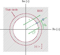
A pole and a zero that have the relationship shown in Fig. 8.41 are said to be mirror images of each other across the unit circle. To find H (Ω) we will evaluate the z-domain system function on the unit circle of the z-plane:
For convenience we will determine the squared magnitude of H (Ω):
The magnitude of the system function is |H (Ω)| = r. It can be shown (see Problem 8.40 at the end of this chapter) that the phase of the system function is
The phase characteristic ∠H (Ω) is shown in Fig. 8.42 for the case of a pole and a zero both on the real axis, that is, for Ω0 = 0. The phase is shown for r = 2.5, r = 1.75 and r = 1.2.

The phase characteristic of the first-order allpass system for Ω0 = 0 and (a) r = 2.5, (b)r = 1.75, (c)r = 1.2.
Since the shape of the phase response can be controlled by the choice of r while keeping the magnitude response constant, an allpass system is also referred to as a phase-shifter. Increased versatility in controlling the phase response can be obtained by choosing the pole and the zero to be complex-valued. This requires Ω0 ≠ 0. Consider a first-order system with a pole at p1 =(1/r)ejΩ0 and a zero at z1 = re jΩ0. Again we choose r > 1 to obtain a system that is both causal and stable. Fig. 8.43 illustrates the phase response ∠H (Ω) is shown for Ω0 = π/6 and Ω0 = π/ 3. The parameter r is fixed at r = 1.2 in both cases.

The phase characteristic of the first-order allpass system for r = 1.2 and (a) Ω0 = π/6, (b) Ω0 = π/3.
If a system function with real-valued coefficients is desired, two first-order allpass sections with complex conjugate zeros and poles can be combined into a second-order allpass system. The resulting system function is
Pole-zero diagram for a second-order allpass system with parameters r and Ω0 is shown in Fig. 8.44.
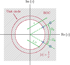
8.5.8 Inverse systems
The inverse of the system is another system which, when connected in cascade with the original system, forms an identity system. This relationship is depicted in Fig. 8.45.
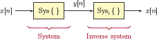
The output signal of the original system is
We require the inverse system to recover the original input signal x[n] from the output signal y [n], therefore
Combining Eqns. (8.273) and (8.273) yields
Let the original system under consideration be a DTLTI system with impulse response h[n], and let the inverse system be also a DTLTI system with impulse response hi[n] as shown in Fig. 8.46. For the output signal of the inverse system to be identical to the input signal of the original system we need the impulse response of the cascade combination to be equal to δ [n], that is,
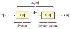
or, using the convolution summation
Corresponding relationship between the system functions is found by taking the z-transform of Eqn. (8.276):
Consequently, the system function of the inverse system is
Two important characteristics of the inverse system are causality and stability. We will first focus on causality. Consider again a rational system function in the standard form
The system function for the inverse system is
If the original system with system function H (z) is causal then M ≤ N as we have established in Section 8.5.5. By the same token, causality of the inverse system with system function H i (z) requires N ≤ M. Hence we need N = M if both the original system and its inverse are required to be causal.
To analyze the stability of the inverse system we will find it more convenient to write the system function H (z) in pole zero form. Using M = N we have
If the original system is both causal and stable, all its poles must be inside the unit circle of the z-plane (see Section 8.5.6), therefore
The system function of the inverse system, written in pole-zero form, is
For the inverse system to be stable, its poles must also lie inside the unit circle. The poles of the inverse system are the zeros of the original system. Therefore, for the inverse system to be stable, both zeros and poles of the original system must be inside the unit circle. In addition to Eqn. (8.282) we also need
A causal DTLTI system that has all of its zeros and poles inside the unit circle is referred to as a minimum-phase system. A minimum-phase system and its inverse are both causal and stable.
Example 8.40: Inverse of a system described by a difference equation
A DTLTI system is described by a difference equation
Determine if a causal and stable inverse can be found for this system. If yes, find a difference equation for the inverse system.
Solution: The system function is found by taking the z-transform of the difference equation and solving for the ratio of the z-transforms of the output signal and the input signal:
The zeros of the system function are at z1 = 0 and z2 = −0.5. Its two poles are at p1 = −0.8 and p2 = 0.9. Since all poles and zeros are inside the unit circle of the z-plane, H(z) is a minimum phase system. The system function for the inverse system is
which is clearly causal and stable. Its corresponding difference equation is
8.6 Implementation Structures for DTLTI Systems
Block diagram implementation of discrete-time systems was briefly discussed in Section 3.6 of Chapter 3. A method was presented for obtaining a block diagram from a linear constant-coefficient difference equation. Three types of elements were utilized; namely signal adder, constant-gain multiplier and one-sample delay. In this section we will build on the techniques presented in Section 3.6, this time utilizing the z-domain system function as the starting point.
8.6.1 Direct-form implementations
The general form of the z-domain system function for a DTLTI system is
For the sake of convenience we chose to write H (z) in terms of negative powers of z. X (z) and Y (z) are the z-transforms of the input and the output signals respectively.
The method of obtaining a block diagram from a z-domain system function will be derived using a third-order system, but its generalization to higher-order system functions is quite straightforward. Consider a DTLTI system for which M = 3 and N = 3. The system function H (z) is
Let us use an intermediate transform V (z) that corresponds to an intermediate signal v [n], and express the system function as
We will elect to associate V (z)/X (z) with the numerator polynomial, that is,
To satisfy Eqn. (8.287), the ratio Y (z)/V (z) must be associated with the denominator polynomial.
The relationships described by Eqns. (8.286) through (8.289) are illustrated in Fig. 8.47.
![]()
(a) DTLTI system with system function H (z), (b) cascade form using an intermediate function V (z).
Solving Eqn. (8.288) for V (z) results in
Taking the inverse z-transform of each side of Eqn. (8.290) and remembering that multiplication of the transform by z−k corresponds to a delay of k samples in the time domain, we get
The relationship between X (z) and V (z) can be realized using the block diagram shown in Fig. 8.48(a). The second part of the system will be implemented by expressing the output transform Y (z) in terms of the intermediate transform V (z). From Eqn. (8.289) we write
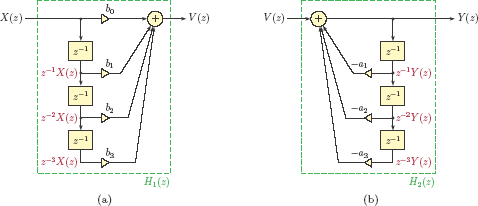
The corresponding time-domain relationship is
The relationship between V (z) and Y (z) can be realized using the block diagram shown in Fig. 8.48(b).
The two block diagrams obtained for H1 (z) and H2 (z) can be connected in cascade as shown in Fig. 8.49 to implement the system function H (z). This is the direct-form I realization of the system.

The block diagram in Fig. 8.49 represents the functional relationship between X (z) and Y (z), the z-transforms of the input and the output signals. If a diagram using time-domain quantities is desired, the conversion is easy using the following steps:
- Replace each transform X (z), Y (z) and V (z) with its time-domain version x [n], y [n] and v [n].
- Replace each block with the factor z −1 with one-sample time delay.
The resulting diagram is shown in Fig. 8.50.

Example 8.41: Direct-form type-I implementation of a system
Consider a causal DTLTI system described by the z-domain system function
Draw a direct-form I block diagram for implementing this system.
Solution: Let us multiply both the numerator and the denominator by z −4 to write the system function in the standard form of Eqn. (8.285):
We have
The block diagram is shown in Fig. 8.51.

Let us consider the direct-form I diagram in Fig. 8.49 again. The subsystem with system function H1 (z) takes X (z) as input, and produces V (z). The subsystem with system function H2 (z) takes V (z), the output of the first subsystem, and produces Y (z) in response. Since each subsystem is linear,2 it does not matter which one comes first in a cascade connection. An alternative way of connecting the two subsystems is shown in Fig. 8.52, and it leads to the block diagram shown in Fig. 8.53.
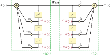
The middle part of the diagram in Fig. 8.53 has two delay lines running parallel to each other, each set containing four nodes. These two sets of nodes hold identical values W (z), z−1 W (z), z −2 W (z) and z −3 W (z). Consequently, the two sets of nodes can be merged together to result in the diagram shown in Fig. 8.54. This is the direct-form II realization of the system.
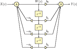
The block diagram in Fig. 8.54 could easily have been obtained directly from the system function in Eqn. (8.286) by inspection, using the following set of rules:
- Begin by ordering terms of numerator and denominator polynomials in ascending powers of z −1.
- Ensure that the leading coefficient in the denominator, that is, the constant term, is equal to unity. (If this is not the case, simply scale all coefficients to satisfy this rule.)
- Set gain factors of feed-forward branches equal to the numerator coefficients.
- Set gain factors of feedback branches equal to the negatives of the denominator coefficients.
- Be careful to account for any missing powers of z −1 in either polynomial, and treat them as terms with their coefficients equal to zero.
Example 8.42: Direct-form II implementation of a system
Draw a direct-form II block diagram for implementing the system used in Example 8.41.
Solution: The diagram obtained by interchanging the order of the two subsystems in Fig. 8.51 and eliminating the nodes that become redundant is shown in Fig. 8.55.

8.6.2 Cascade and parallel forms
Instead of simulating a system with the direct-form block diagram discussed in the previous section, it is also possible to express the system function as either the product or the sum of lower order sections, and base the block diagram on cascade of parallel combination of smaller diagrams. Consider a system function of order M that can be expressed in the form
One method of simulating this system would be to build a diagram for each of the subsections Hi (s) using the direct-form approach discussed previously, and then to connect those sections in cascade as shown in Fig. 8.56.
An easy method of sectioning a system function in the style of Eqn. (8.294) is to first find the poles and the zeros of the system function, and then use them for factoring numerator and denominator polynomials. Afterwards, each section may be constructed by using one of the poles. Each zero is incorporated into one of the sections, and some sections may have constant numerators. If some of the poles and zeros are complex-valued, we may choose to keep conjugate pairs together in second-order sections to avoid the need for complex gain factors in the diagram. The next example will illustrate this process.
Example 8.43: Cascade form block diagram
Develop a cascade form block diagram for the DTLTI system used in Example 8.41.
Solution: The system function specified in Example 8.41 has zeros at z1 = −3, z2 = 2, z3 = 1, and poles at p1 = −0.9, p2 = 0.3, p3, 4 = 0.8 ± j 0.5 (see MATLAB Exercise 8.9). It can be written in factored form as
The system function can be broken down into cascade sections in a number of ways. Let us choose to have two second-order sections by defining (see MATLAB Exercise 8.9)
and
so that
A cascade form block diagram is obtained by using direct-form II for each of H1 (z) and H2 (z), and connecting the resulting diagrams as shown in Fig. 8.57.
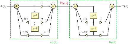
It is also possible to consolidate the neighboring adders in the middle although this would cause the intermediate signal W1 (z) to be lost. The resulting diagram is shown in Fig. 8.58.
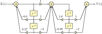
Software resources: |
See MATLAB Exercises 8.9 and 8.10. |
An alternative to the cascade form simulation diagram is a parallel form diagram which is based on writing the system function as a sum of lower order functions:
A simulation diagram may be constructed by implementing each term in Eqn. (8.295) using the direct-form approach, and then connecting the resulting subsystems in a parallel configuration as shown in Fig. 8.59.

A rational system function H (z) may be sectioned in the form of Eqn. (8.295) using partial fraction expansion. If some of the poles and zeros are complex-valued, we may choose to keep conjugate pairs together in second-order sections to avoid the need for complex gain factors in the diagram. This process will be illustrated in the next example.
Example 8.44: Parallel form block diagram
Develop a cascade form block diagram for the DTLTI system used in Example 8.41.
Solution: The system function has poles at p1 = −0.9, p2 = 0.3and p3, 4 = 0.8 ± j 0.5. Let us expand it into partial fractions in the form
Note that it is not necessary to divide H (z) by z before expanding it into partial fractions since we are not trying to compute the inverse transform. The residues of the partial fraction expansion are (see MATLAB Exercise 8.11)
and H (s) is
Let us combine the first two terms to create a second-order section:
The remaining two terms are combined into another second-order section, yielding
so that
The parallel form simulation diagram is shown in Fig. 8.60.
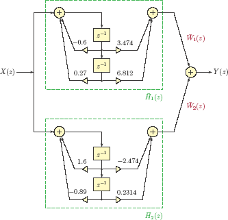
Software resources: |
See MATLAB Exercise 8.11. |
8.7 Unilateral z-Transform
It was mentioned in earlier discussion that the z-transform as defined by Eqn. (8.1) is often referred to as the bilateral z-transform. An alternative version, known as the unilateral z-transform, is defined by
We use the subscript “u” to distinguish the unilateral z-transform from its bilateral counterpart. It is clear from a comparison of Eqn. (8.296) with Eqn. (8.1) that the only difference between the two definitions is the lower index of the summation. In Eqn. (8.296) we start the summation at n = 0 instead of n = ∞. If x [n] is a causal signal, that is, if x [n]= 0 for n < 0, then the unilateral transform X u (z) becomes identical to the bilateral transform X (z). On the other hand, for a signal that is x [n] is not necessarily causal, the unilateral transform is essentially the bilateral transform of x [n] multiplied by a unit-step function, that is,
Because of the way X u (z) is defined, its region of convergence is always the outside of a circle, and does not have to be explicitly stated.
One property of the unilateral z-transform that differs from its counterpart for the bilateral z-transform is the time-shifting property. Consider the time-shifted signal x [n − 1]. In terms of the bilateral z-transform, we have proved the following relationship in earlier discussion:
The relationship in Eqn. (8.298) does not extend to the unilateral z-transform, that is, we cannot claim that Ƶ u{x [n − 1]} = z −1 Z u{x [n]}. The reason for this fundamental difference becomes obvious if we write the unilateral transform in open form:
The transform of the time-shifted signal is
The sample x [−1] is not part of Z u{x [n]} but appears in Z u{x [n − 1]}. Let us rewrite the latter by separating x [−1] from the rest of the terms:
Consequently, the unilateral z-transform of x [n − 1] can be expressed in terms of the transform of x [n] as
Through similar reasoning it can be shown that, for the signal x [n − 2], we have
and in the general case of a signal time-shifted by k > 0 samples
If the signal is advanced rather than delayed in time, it can be shown that (see Problem 8.44 at the end of this chapter)
for k > 0. The unilateral z-transform is useful in the use of z-transform techniques for solving difference equations with specified initial conditions. The next couple of examples will illustrate this.
Example 8.45: Finding the natural response of a system through z-transform
The homogeneous difference equation for a system is
Using z-transform techniques, determine the natural response of the system for the initial conditions
Recall that this problem was solved in Example 3.12 of Chapter 3 using time-domain solution techniques.
Solution: The first step will be to compute the unilateral z-transform of both sides of the homogeneous difference equation:
Using the linearity of the z-transform we can write
The unilateral z-transforms of the time-shifted versions of the output signal are
and
Substituting Eqns. (8.307) and (8.308) into Eqn. (8.306) we get
which can be solved for Y u (z) to yield
Now we need to find y [n] through inverse z-transform using partial fraction expansion. We will write Y u (z) as
The residues of the partial fraction expansion are
Thus, the partial fraction expansion for Y u (z) is
resulting in the homogeneous solution
This result is in perfect agreement with that found in Example 3.12.
Software resources: |
See MATLAB Exercise 8.13. |
Example 8.46: Finding the forced response of a system through z-transform
Consider a system defined by means of the difference equation
Determine the response of this system for the input signal
if the initial value of the output is y [−1] = 2.5. Recall that this problem was solved in Example 3.15 of Chapter 3 using time-domain solution techniques.
Solution: Let us begin by computing the unilateral z-transform of both sides of the difference equation.
In Example 8.15 we have found
Adapting that result to the transform of the input signal x [n] given, we get
The unilateral z-transform of the y [n − 1] term is
Substituting Eqns. (8.311) and (8.312) into Eqn. (8.309) we obtain
from which the unilateral z-transform of the output signal can be obtained as
We are now ready to determine y [n] using partial fraction expansion. Let
The residues are
and
The third residue, k3, can be computed in a similar manner, however, we will take a shortcut and recognize the fact that complex residues of a rational transform must occur in complex conjugate pairs provided that all coefficients of the denominator polynomial are real-valued. Consequently we have
It will be more convenient to express k2 and k3 in polar complex form as
The forced response of the system is
or equivalently
which is consistent with the answer found earlier in Example 3.15.
8.8 Further Reading
[1] U. Graf. Applied Laplace Transforms and Z-Transforms for Scientists and Engineers: A Computational Approach Using a Mathematica Package. Birkhäuser, 2004.
[2] D.G. Manolakis and V.K. Ingle. Applied Digital Signal Processing: Theory and Practice. Cambridge University Press, 2011.
[3] A.V. Oppenheim and R.W. Schafer. Discrete-Time Signal Processing. Prentice Hall, 2010.
[4] R.A. Schilling, R.J. Schilling, and P.D. Sandra L. Harris. Fundamentals of Digital Signal Processing Using MATLAB. Cengage Learning, 2010.
[5] L. Tan and J. Jiang. Digital Signal Processing: Fundamentals and Applications. Elsevier Science, 2013.
MATLAB Exercises
MATLAB Exercise 8.1: Three-dimensional plot of z-transform
In Fig. 8.3 the magnitude of the transform
Eqn. (8.9):
was graphed as a three-dimensional surface. In this exercise we will reproduce that figure using MATLAB, and develop the code to evaluate and display the transform on a circular trajectory z = re jΩ. The first step is to produce a set of complex values of z on a rectangular grid in the z-plane.
>> [zr, zi] = meshgrid ([-1.5:0.03:1.5], [-1.5:0.03:1.5]);
>> z = zr+j*zi ;
The next step is to compute the magnitude of the z-transform at each point on the grid. An anonymous function will be used for defining X (z). Additionally, values of magnitude that are greater than 12 will be clipped for graphing purposes.
>> Xz = @(z) z.*(z-0.7686)./(z.*z-1.5371*z+0.9025);
>> XzMag = abs (Xz (z));
>> XzMag = XzMag .*(XzMag <=12)+12.*(XzMag >12);
A three-dimensional mesh plot of |X (z)| plot can be generated with the following lines:
>> mesh (zr , zi , XzMag);
>> axis ([-1.5 , 1.5 , -1.5 , 1.5]);
The script listed below produces a mesh plot complete with axis labels and color specifications.
1 % Script : matex_8_1a.m
2 %
3 [zr , zi] = meshgrid ([-1.5:0.03:1.5] , [-1.5:0.03:1.5]);
4 z = zr+j*zi;
5 Xz = @(z) z .*(z -0.7686)./(z .*z -1.5371* z +0.9025); % Eqn .(8.9)
6 XzMag = abs (Xz(z));
7 XzMag = XzMag .*(XzMag <=12)+12.*(XzMag >12);
8 shading interp ; % Shading method : Interpolated
9 colormap copper ; % Specify the color map used.
10 m1 = mesh (zr ,zi , XzMag);
11 axis ([-1.5 ,1.5 , -1.5 , 1.5]);
12 % Adjust transparency of surface lines.
13 set (m1 , ’EdgeAlpha’ ,0.6’, ’ FaceAlpha ’ ,0.6);
14 % Specify x,y,z axis labels.
15 xlabel (’Re [z]’);
16 ylabel (’Im [z]’);
17 zlabel (’|X(z)| ’);
18 % Specify viewing angles.
19 view (gca ,[56.5 40]);
In line 10 of the script, the handle returned by the function mesh(..) is assigned to the variable m1 so that it can be used in line 13 for adjusting the transparency of the surface.
The DTFT X (Ω) is equal to the z-transform evaluated on the unit circle of the z-plane, that is,
Applying this relationship to the magnitudes of the two transforms, the magnitude of the DTFT is obtained by evaluating the magnitude of the z-transform on the unit circle. The script listed below demonstrates this.
1 % Script : matex_8_1b.m
2 %
3 [zr , zi] = meshgrid ([-1.5:0.03:1.5] ,[-1.5:0.03:1.5]);
4 z = zr+j*zi;
5 Xz = @(z) z .*(z -0.7686)./(z .*z -1.5371* z +0.9025); % Eqn. (8.9)
6 XzMag = abs (Xz(z));
7 XzMag = XzMag .*(XzMag <=12)+12.*(XzMag >12);
8 % Set the trajectory.
9 r = 1; % Radius of the trajectory.
10 Omega = [0:0.005:1]*2* pi;
11 tr = r* exp (j* Omega);
12 % Produce a mesh plot and hold it.
13 shading interp ; % Shading method : Interpolated
14 colormap copper ; % Specify the color map used.
15 m1 = mesh (zr ,zi , XzMag);
16 set (m1 , ’ EdgeAlpha ’ ,0.6’, ’ FaceAlpha ’ ,0.6);
17 hold on;
18 % Superimpose a plot of X(z) magnitude values evaluated
19 % on the trajectory using ’ plot3 ’ function.
20 m2 = plot3 (real (tr), imag (tr), abs (Xz(tr)), ’b -’,’ LineWidth ’ ,1.5);
21 % Show the unit - circle in red.
22 m3 = plot3 (real (tr), imag (tr), zeros (size (tr)), ’r- ’,’ LineWidth ’ ,1.5);
23 hold off ;
24 axis ([-1.5 ,1.5 , -1.5 ,1.5]);
25 % Specify x,y,z axis labels.
26 xlabel (’Re [z] ’);
27 ylabel (’Im [z] ’);
28 zlabel (’|X(z)| ’);
29 % Specify viewing angles.
30 view (gca ,[56.5 40]);
Software resources:
matex_8_1a.m
matex_8_1b.m
MATLAB Exercise 8.2: Computing the DTFT from the z-transform
The DTFT of a signal is equal to its z-transform evaluated on the unit circle of the z-plane.
Consider the z-transform
The first method of computing and graphing the DTFT of the signal is to use an anonymous function for X (z) and evaluate it on the unit circle. The magnitude |X (Ω)| is graphed using the following statements:
>> X = @(z) (z -0.7686)./(z.*z -1.5371* z +0.9025);
>> Omg = [-1:0.001:1]* pi ;
>> Xdtft = X(exp (j* Omg));
>> plot (Omg , abs (Xdtft)); grid ;
If the phase ∡X (Ω) is needed, it can be graphed using
>> plot (Omg , angle (Xdtft)); grid ;
The second method is to use MATLAB function freqz(..). Care must be taken to ensure that the function is used with proper arguments, or erroneous results may be obtained. The function freqz(..) requires that the transform X (z) be expressed using negative powers of z in the form
Vectors "num" and "den" to hold numerator and denominator coefficients should be entered as
>> num = [0 ,1 , -0.7686];
>> den = [1 , -1.5371 ,0.9025];
Afterwards the magnitude and the phase of the DTFT can be computed and graphed with the statements
>> Omg = [-1:0.001:1]* pi ;
>> [Xdtft , Omg] = freqz (num ,den , Omg);
>> plot (Omg , abs (Xdtft)); grid ;
>> plot (Omg , angle (Xdtft)); grid ;
Common mistake: Pay special attention to the leading 0 in the numerator coefficient vector. Had we omitted it, the function freqz(..) would have incorrectly used the transform
resulting in the correct magnitude |X (Ω)| but incorrect phase ∡X (Ω). This example demonstrates the potential for errors when built-in MATLAB functions are used without carefully reading the help information.
Software resources:
matex_8_2a.m
matex_8_2b.m
MATLAB Exercise 8.3: Graphing poles and zeros
Consider a DTLTI system described by the system function
Poles and zeros of the system function can be graphed on the z-plane by entering coefficients of numerator and denominator polynomials as vectors and then computing the roots.
>> num = [1 ,0 , -0.5 ,0.5];
>> den = [1 , -0.5 , -0.5 , -0.6 ,0.6];
>> z = roots (num);
>> p = roots (den);
To produce the graph we need
>> plot (real (z), imag (z),’o’, real (p), imag (p), ’x ’);
which uses "o" for azeroand "x" for a pole. The graph produced does not display the unit circle of the z-plane, and the aspect ratio may not be correct. These issues are resolved using the code below:
>> Omg = [0:0.001:1]*2* pi;
>> c = exp (j* Omg); % Unit circle
>> plot (real (z), imag (z),’o’, real (p), imag (p), ’x ’,real (c), imag (c), ’: ’);
>> axis equal
Alternatively, built-in function zplane(..) may be used for producing a pole-zero plot, however, caution must be used as in the previous MATLAB exercise. The function zplane(..) expects numerator and denominator polynomials to be specified in terms of negative powers of z. Using the vectors "num" and "den" as entered above and calling the function zplane(..) through
>> zplane (num , den);
would display an incorrect pole-zero plot with an additional zero at the origin. The correct use for this problem would be
>> num = [0 ,1 ,0 , -0.5 ,0.5];
>> den = [1 , -0.5 , -0.5 , -0.6 ,0.6];
>> zplane (num , den);
Software resources:
matex_8_3a.m
matex_8_3b.m
MATLAB Exercise 8.4: Using convolution function for polynomial multiplication
The function conv(..) for computing the convolution of two discrete-time signals was used in MATLAB Exercise 3.7 in Chapter 3. In Example 8.23 of this chapter we have discovered another interesting application of the conv(..) function, namely the multiplication of two polynomials. In this exercise we will apply this idea to the multiplication of the two polynomials
and
The problem is to determine the polynomial C (v)= A (v)B (v). We will begin by creating a vector with the coefficients of each polynomial ordered from highest power of v down to the constant term, being careful to account for any missing terms:
>> A = [5 ,7 ,0 ,3 , -2]; % Coefficients a_4 , ... , a_0
>> B = [8, 6 ,-3, 1, -4, 2]; % Coefficients b_5 , ... , b_0
For the convolution operation the coefficients are needed in ascending order starting with the constant term. MATLAB function fliplr(..) will be used for reversing the order.
>> tmpA = fliplr (A); % Coefficients a_0 , ... , a_4
>> tmpB = fliplr (B); % Coefficients b_0 , ... , a_5
>> tmpC = conv (tmpA , tmpB); % Coefficients c_0 , ... , a_9
>> C = fliplr (tmpC) % Coefficients c_9 , ... , c_0
C =
40 86 27 8 -11 -39 23 -14 14 -4
The product polynomial is
Software resources:
matex_8_4.m
MATLAB Exercise 8.5: Partial fraction expansion with MATLAB
Find a partial fraction expansion for the transform
Solution: We need to create two vectors "num" and "den" with the numerator and the denominator coefficients of X (z)/z and then use the function residue(..). The statements below compute the z-domain poles and residues:
>> num = [-0.2000 ,1.8200 , -3.5900 ,3.1826];
>> den = [1.0000 , -1.2000 ,0.4600 ,0.4520 , -0.5607 ,0];
>> [r,p,k] = residue (num , den)
r =
0.8539 + 0.0337 i
0.8539 - 0.0337 i
1.1111
2.8571
-5.6761
p =
0.5000 + 0.8000 i
0.5000 - 0.8000 i
0.9000 -0.7000
0
k =
[]
Based on the results obtained, the PFE is in the form
or, equivalently
Software resources:
matex_8_5.m
MATLAB Exercise 8.6: Developing a function for long division
In this exercise we will develop a MATLAB function named "ss_longdiv" to compute the inverse z-transform by long division. MATLAB function deconv(..) will be used for implementing each step of the long division operation. The utility function ss_longdiv_util(..) listed below implements one step of the long division.
1 function [q,r] = ss_longdiv_util(num ,den)
2 M = max (size (num)) -1; % The order of the numerator.
3 N = max (size (den)) -1; % The order of the denominator.
4 % Append the shorter vector with zeros.
5 if (M < N)
6 num = [num , zeros (1,N -M)];
7 elseif (M > N)
8 den = [den , zeros (1,M -N)];
9 end ;
10 [q ,r] = deconv (num , den); % Find quotient and remainder.
11 r = r (2: length (r)); % Drop first element of remainder
12 % which is 0.
13 end
To test this function, let us try the transform in Example 8.31.
The first sample of the inverse transform is obtained using the following:
>> num = [3 , -1 ,0];
>> den = [1,-3,3,-1];
>> [q,r] = ss_longdiv_util(num ,den)
q =
3
r =
8 -9 3
This result should be compared to Eqn. (8.208). The next step in the long division can be performed with the statement
>> [q,r] = ss_longdiv_util(r,den)
q =
8
r =
15 -21 8
and matches Eqn. (8.209). This process can be repeated as many times as desired. The function ss_longdiv(..) listed below uses the function ss_longdiv_util(..) in a loop to compute n samples of the inverse transform.
1 function [x] = ss_longdiv (num , den , n)
2 [q,r] = ss_longdiv_util(num , den);
3 x = q;
4 for nn = 2:n ,
5 [q,r] = ss_longdiv_util(r, den);
6 x = [x , q];
7 end;
8 end
It can be tested using the problem in Example 8.31:
>> x = ss_longdiv ([3 , -1 , 0] , [1 , -3 , 3 , -1] , 6)
x =
3 8 15 24 35 48
If a left-sided result is desired, the function ss_longdiv(..) can be still be used by simply reordering the coefficients in the vectors “num” and “den”. Refer to the transform in Example 8.32.
The left-sided solution is obtained by
>> num = fliplr ([1 , 1 , -2]);
>> den = fliplr ([1 , -2.5 , 1]);
>> x = ss_longdiv (num , den , 6)
x =
-2.0000 -4.0000 -7.0000 -13.5000 -26.7500 -53.3750
ss_longdiv.m
ss_longdiv_util.m
MATLAB Exercise 8.7: Computing frequency response of a system from pole-zero layout
The problem of obtaining the frequency response of a DTLTI system from the placement of its poles and zeros in the z-domain was discussed in Section 8.5.4. In this exercise we will use MATLAB to compute the frequency response for a system characterized by the system function
The system has one zero at z = −0.6 and one pole at z = 0.8. Suppose we need the frequency response of this system at the angular frequency of Ω = 0.3π radians, which is equal to the system function evaluated at z = ej0.3π:
Using vector notation, we have
where we have defined the vectors and for notational convenience. The script listed below computes the vectors and and uses them for computing the magnitude and the phase of the system function at ω = 0.3π:
1 % Script : matex_8_7a.m
2 %
3 Omega = 0.3* pi;
4 z = exp (j* Omega);
5 B = z +0.6;
6 A = z -0.8;
7 mag = abs (B)/ abs (A);
8 phs = angle (B)- angle (A);
This script computes the frequency response of the system at one specific frequency. It would be more interesting if we could use the same idea to compute the frequency response of the system at a large number of angular frequencies so that its magnitude and phase can be graphed as functions of Ω. Let us change the variable “Omega” into a vector by editing line 1 of the script:
1 Omega = [-1:0.004:1]* pi;
This change causes the variable “z” to become a complex vector with 501 elements. Also, in line 5, the standard division operator “/” needs to be changed to the element-by-element division operator “./” to read
5 mag = abs (B)./ abs (A);
The MATLAB script is listed below with these modifications and the addition of graphing statements:
1 % Script : matex_8_7b.m
2 %
3 Omega = [-1:0.004:1]* pi;
4 z = exp (j* Omega);
5 B = z +0.6;
6 A = z -0.8;
7 mag = abs (B)./ abs (A);
8 phs = angle (B)- angle (A);
9 clf;
10 subplot (2 , 1 , 1);
11 plot (Omega , mag);
12 title (’ Magnitude of the frequency response ’);
13 xlabel (’ Omega (rad)’); grid;
14 subplot (2 , 1 , 2);
15 plot (Omega , phs);
16 title (’ Phase of the frequency response ’);
17 xlabel (’ Omega (rad)’); grid;
Software resources:
matex_8_7a.m
matex_8_7b.m
MATLAB Exercise 8.8: Frequency response from pole-zero layout revisited
In MATLAB Exercise 8.7 we have explored a method of computing the frequency response of a DTLTI system based on the graphical interpretation of the pole-zero layout of the system function, discussed in Section 8.5.4. The idea can be generalized into the development of a MATLAB function ss_freqz(..) for computing the frequency response.
1 function [mag , phs] = ss_freqz (zrs ,pls , gain , Omega)
2 nz = length (zrs); % Number of zeros.
3 np = length (pls); % Number of poles.
4 nOmg = length (Omega); % Number of frequency points.
5 z = exp (j* Omega); % Get points on the unit - circle.
6 mag = ones (1, nOmg);
7 phs = zeros (1, nOmg);
8 if (nz > 0) ,
9 for n = 1: nz
10 mag = mag .* abs (z - zrs (n));
11 phs = phs + angle (z - zrs (n));
12 end;
13 end;
14 if (np > 0) ,
15 for n = 1: np
16 mag = mag ./ abs (z - pls (n));
17 phs = phs - angle (z - pls (n));
18 end;
19 end;
20 mag = mag * gain;
21 phs = wrapToPi (phs);
Line 21 of the function causes phase angles to be contained in the interval (−π, π). The script listed below may be used for testing ss_freqz(..) with the system function
1 % Script : matex_8_8.m
2 %
3 num = [1 , -0.7686];
4 den = [1 , -1.5371 ,0.9025];
5 zrs = roots (num); % Compute zeros.
6 pls = roots (den); % Compute poles.
7 Omg = [-1:0.001:1]* pi; % Vector of frequencies.
8 [mag , phs] = ss_freqz (zrs ,pls ,1, Omg);
9 clf;
10 subplot (2 ,1 ,1);
11 plot (Omg , mag); grid;
12 xlabel (’ Omega (rad)’);
13 subplot (2 ,1 ,2);
14 plot (Omg , phs); grid;
15 xlabel (’ Omega (rad)’);
Software resources:
ss_freqz.m
matex_8_8.m
MATLAB Exercise 8.9: Preliminary calculations for a cascade-form block diagram
In this exercise we will use MATLAB to help with the preliminary calculations for sectioning a system function into cascade subsystems to facilitate the development of a cascade-form block diagram.
Consider the system function first used in Example 8.41.
A cascade-form block diagram was obtained in Example 8.43. Two vectors “num” and “den” are created with the following statements to hold numerator and denominator coefficients in descending powers of z:
>> num=[1,0,-7,6];
>> den =[1 , -1 , -0.34 ,0.966 , -0.2403];
Poles and zeros of the system function are found as
>> z = roots (num)
z =
-3.0000
2.0000
1.0000
>> p = roots (den)
p =
-0.9000
0.8000 + 0.5000 i
0.8000 - 0.5000 i
0.3000
The returned vector “z” holds the three zeros of the system function that are all real-valued. The vector “p” holds the four poles. The first subsystem H1 (z) will be formed using zeros #1 and #3 along with poles #1 and #4. Using the function poly(..) for polynomial construction from roots, the numerator and denominator coefficients of H (z) are obtained as
>> num1 = poly ([z(1) , z (3)])
num1 =
1.0000 2.0000 -3.0000
>> den1 = poly ([p(1) , p (4)])
den1 =
1.0000 0.6000 -0.2700
corresponding to
The remaining zero will be combined with poles #2 and #3 to yield the numerator and the denominator of H2 (z):
>> num2 = [1,- z (2)]
num2 =
1.0000 -2.0000
>> den2 = poly ([p(2) , p (3)])
den2 =
1.0000 -1.6000 0.8900
The second subsystem is therefore
Software resources:
matex_8_9.m
MATLAB Exercise 8.10: Preliminary calculations for a cascade-form block diagram revisited
An alternative method of breaking up a system function into second-order cascade sections is to use MATLAB functions tf2zp(..) and zp2sos(..). Working with the same system function as in MATLAB Exercise 8.9 use the following set of statements:
>> num = [0 ,1 ,0 , -7 ,6];
>> den = [1 , -1 , -0.34 ,0.966 , -0.2403];
>> [z,p ,k] = tf2zp (num , den);
>> [sos ,G] = zp2sos (z ,p,k)
sos =
0 1.0000 3.0000 1.0000 0.6000 -0.2700
1.0000 -3.0000 2.0000 1.0000 -1.6000 0.8900
G =
1
It is important to remember that vectors “num” and “den” hold coefficients of numerator and denominator polynomials in terms of ascending negative powers of z. In general they need to be of the same length, hence requiring a zero-valued element to be added in front of the vector “num”. Second-order sections are in the form
Each row of the matrix “sos” holds coefficients of one second-order section in the order
The result obtained above corresponds to second-order sections
and
Software resources:
matex_8_10.m
MATLAB Exercise 8.11: Preliminary calculations for a parallel-form block diagram
This exercise is about using MATLAB to help with the preliminary calculations for sectioning a system function into parallel subsystems to facilitate the development of a parallel-form block diagram.
Consider again the system function first used in Example 8.41.
A parallel-form block diagram was obtained in Example 8.44. In order to obtain the subsystems and for the parallel-form implementation we will begin by creating vectors “num” and “den” to hold numerator and denominator coefficients in descending powers of z:
>> num=[1,0,-7,6];
>> den =[1 , -1 , -0.34 ,0.966 , -0.2403];
Residues are found using the function residue(..). Recall from the discussion in MATLAB Exercise 8.5 that there is also a function named residuez(..) specifically designed for z-domain residues. However, it utilizes a slightly different format than the conventions we have developed in Section 8.4.2 for the partial fraction expansion, and therefore will not be used here.
>> [r,p,k] = residue (num , den)
r =
-1.2371 + 1.7480 i
-1.2371 - 1.7480 i
-3.0709
6.5450
p =
0.8000 + 0.5000 i
0.8000 - 0.5000 i
-0.9000
0.3000
k =
[]
We will recombine the two terms with real poles (terms #3 and #4 in the lists of poles and residues computed by MATLAB) to obtain :
>> [num1 , den1] = residue (r (3:4) , p (3:4) ,[]);
>> H1 = tf (num1 , den1 , -1)
Transfer function :
3.474 z + 6.812
------------------
z ^2 + 0.6 z - 0.27
Sampling time : unspecified
The remaining terms (items #1 and #2) will be recombined for the second subsystem :
>> [num2 , den2] = residue (r (1:2) , p (1:2) ,[]);
>> H2 = tf (num2 , den2 , -1)
Transfer function :
-2.474 z + 0.2314
------------------
z ^2 - 1.6 z + 0.89
Sampling time : unspecified
so that
To see if this is indeed the case, let us add the two system functions:
>> H = H1 +H2
Transfer function :
z ^3 - 8.882 e -016 z ^2 - 7 z + 6
--------------------------------------------
z ^4 - z ^3 - 0.34 z^2 + 0.966 z - 0.2403
Sampling time : unspecified
Software resources:
matex_8_11.m
MATLAB Exercise 8.12: Implementing a system using second-order sections
In Section 8.6.2 cascade and parallel implementation forms of a rational system function H (z) were discussed using second-order sections.
The second-order rational system function
may be used as the basis of cascade and parallel implementations, and may be implemented using the direct-form II block diagram shown in Fig. 8.61.

We will develop a MATLAB function ss_iir2(..) for a generic implementation of this second-order system. The focus will be on making the function reusable within a larger block diagram implemented in either cascade or parallel form. For flexibility the function takes in one sample of the input signal at a time, and returns one sample of the output signal. The syntax of the function ss_iir2(..) is
[out , states] = ss_iir2 (inp , coeffs , states)
The scalar “inp” is the current sample of the input signal. The vector “coeffs” holds the coefficients of the second-order IIR filter stage in the following order:
Note that this is the same coefficient order used in MATLAB functions tf2sos, zp2sos and ss2sos. Finally, the input vector “states” holds values of the internal variables r1 and r2 set in the previous step:
The return variable “out” is the current output sample computed in response to the current input sample. The function also returns updated values of the internal variables r1 and r2 in the vector “states”. These will be needed the for processing the next input sample.
The listing for the function ss_iir2 is given below:
1 function [out , states] = ss_iir2 (inp , coeffs , states)
2 % Extract the filter states.
3 r1 = states (1);
4 r2 = states (2);
5 % Extract the coefficients.
6 b0 = coeffs (1);
7 b1 = coeffs (2);
8 b2 = coeffs (3);
9 a1 = coeffs (5);
10 a2 = coeffs (6);
11 % Compute the output sample.
12 r0 = inp - a1 *r1 - a2 * r2;
13 out = b0*r0+b1*r1+b2*r2;
14 % Update the filter states : r1 <-r0 , r2 <- r1
15 states (1) = r0;
16 states (2) = r1;
17 end
To test the function, we will use the DTLTI system used in Examples 8.43 and 8.44. The cascade form block diagram shown in Fig. 8.57 may be implemented with the following script that computes and graphs the unit-step response of the system:
1 % Script : matex_8_12a.m
2 %
3 states1 = [0 ,0];
4 states2 = [0 ,0];
5 coeffs1 = [1 ,2 , -3 ,1 ,0.6 , -0.27];
6 coeffs2 = [0 ,1 , -2 ,1 , -1.6 ,0.89];
7 x = ones (1 ,100);
8 y = zeros (1 ,100);
9 for n =1:100 ,
10 inp = x(n);
11 [w1 , states1] = ss_iir2 (inp , coeffs1 , states1);
12 [y(n), states2] = ss_iir2 (w1 , coeffs2 , states2);
13 end;
14 stem ([0:99] , y);
Similarly, the script listed below computes and graphs the unit-step response of the same system using the parallel form block diagram obtained in Example 8.44 and shown in Fig. 8.60.
1 % Script : matex_8_12b.m
2 %
3 states1 = [0 ,0];
4 states2 = [0 ,0];
5 coeffs1 = [0 ,3.474 ,6.812 ,1 ,0.6 , -0.27];
6 coeffs2 = [0 , -2.474 ,0.2314 ,1 , -1.6 ,0.89];
7 x = ones (1 ,100);
8 y = zeros (1 ,100);
9 for n =1:100 ,
10 inp = x(n);
11 [w1 , states1] = ss_iir2 (inp , coeffs1 , states1);
12 [w2 , states2] = ss_iir2 (inp , coeffs2 , states2);
13 y(n) = w1+w2;
14 end;
15 stem ([0:99] , y);
Software resources:
ss_iir2.m
matex_8_12a.m
matex_8_12b.m
MATLAB Exercise 8.13: Solving a difference equation through z-transform
In Section 8.7 two examples of using the unilateral z-transform for solving difference equations with specified initial conditions were given. In this exercise we will use the symbolic processing capabilities of MATLAB to solve the problem in Example 8.45. The functions ztrans(..) and iztrans(..) are available for symbolic computation of the forward and inverse z-transform. They both assume that the time-domain signal involved is causal. In effect they implement the unilateral variant of the z-transform.
Consider the homogeneous difference equation explored in Example 8.45
with the initial conditions
Unilateral z-transforms of y[n − 1] and y[n − 2] are
The following script can be used for solving the problem:
1 % Script : matex_8_13.m
2 %
3 syms z n Yz
4 Y1 = 19+ z ^(-1)* Yz; % z - transform of y[n -1]
5 Y2 = 53+19* z ^(-1)+ z ^(-2)* Yz; % z - transform of y[n -2]
6 Yz = solve (Yz -5/6* Y1 +1/6* Y2 ,Yz); % Solve for Y(z)
7 yn = iztrans (Yz) % Inverse z- transform of Y(z)
In line 3 we declare three symbolic variables. The variable “Yz” corresponds to the yet unknown transform Yu (z). Line 6 of the script uses the function solve(..) to solve the equation
for Yu (z). Line 7 generates the response
yn =
2*(1/2)^ n + 5*(1/3)^ n
which is in agreement with the solution found in Example 8.45. If desired, the symbolic expression in MATLAB variable “yn” may be numerically evaluated and graphed with the following statements:
>> n = [0:10];
>> y = eval (yn);
>> stem (n ,y);
Software resources:
matex_8_13a.m
matex_8_13b.m
Problems
8.1. Using the definition of the z-transform, compute X (z) for the signals listed below. Write each transform using non-negative powers of z. In each case determine the poles and the zeros of the transform, and the region of convergence.
- 8.2. For each transform X (z) listed below, determine whether the DTFT of the corresponding signal x[n] exists. If it does, find it.
- 8.3. Pole-zero diagrams for four transforms are shown in Fig. P.8.3. For each, determine the ROC if it is known that the DTFT of x[n] exists.
- 8.4. Determine the z-transforms of the signals given below. Indicate the ROC for each.
- 8.5. Find the z-transform of the signal

Also indicate the ROC.
- 8.6. Consider the signal g[n] specified as
- Determine the transform G(z) and its ROC.
- Let a new signal x[n] be obtained from g[n] through the relationship x[n] = g[2n]. Determine the transform X (z) and its ROC from the transform G (z) using the development outlined in Example 8.11.
- Determine the transform X (z) and its ROC by direct application of the z-transform definition to the signal x[n]. Compare to the result obtained in part (b).
- 8.7. Determine the z-transform of each signal listed below, and indicate the ROC. Use linearity, time shifting and time reversal properties of the z-transform when needed.
- x[n] = δ[n + 2]
- x[n] = δ[n − 3]
- x[n] = (3)n u[−n − 1]
- x[n] = (3)n u[−n +1]
- 8.8. Consider the signal
- Express x[n] as the sum of a causal signal xR[n] and an anti-causal signal xL[n]. Find an analytical expression for each component, and sketch each component.
- Determine the transforms XR(z) and XL(z) corresponding to the signals xR[n] and xL[n] respectively. Also determine the ROC for each transform.
- Use linearity of the z-transform to express X(z) and to determine its ROC.
- 8.9. Use the time reversal property of the z-transform to determine X(z) for the signals listed below. Indicate the ROC for each.
- x[n] = u[−n]
- x[n] = u[−n − 1]
- x[n] = u[−n] −u[−n − 5]
- x[n] = n u[−n]
- x[n] = cos(Ω0n) u[−n]
- 8.10. Use the differentiation property of the z-transform to find the transform of each signal below. Also indicate the ROC for each.
- 8.11. Transforms of several causal signals are listed below. Use the initial value property of the z transform to determine x[0] for each case.
- 8.12.
Use the correlation property of the z-transform to determine the autocorrelation function for
Hint: Write X (z) in polynomial form.
Generalize the result in part (a) to find the autocorrelation function for
using z-transform techniques.
- 8.13. Use the correlation property of the z-transform to determine the cross correlation function for the signals
and
Hint: Write X (z) and Y (z) in polynomial form.
- 8.14. Prove that the cross correlation of signals x[n] and y[n] is equal to the convolution of x[n] and y[−n], that is,
- Using direct application of the convolution sum
- Using correlation and time reversal properties of the z-transform
- 8.15. Let x[n] = an u[n]. A signal w[n] is defined in terms of x[n] as
- Determine X (z). Afterwards determine W (z) from X (z) using the summation property of the z-transform.
- Determine w[n] from the transform W (z) using partial fraction expansion.
- Determine w[n] directly from the summation relationship using the geometric series formula and compare to the result found in part (b).
8.16. Using the summation property of the z transform prove the well-known formula
Hint: Use x [n] = n u [n] and .
8.17. Consider the z-transforms listed below along with their ROCs. For each case determine the inverse transform x [n] using partial fraction expansion.
8.18. The transform X (z) is given by
The ROC is not specified.
- Construct a pole-zero plot for X (z) and identify all possibilities for the ROC.
- Express X (z) using partial fractions and determine the residues.
- For each choice of the ROC, determine the inverse transform x [n].
8.19. The transforms listed below have complex poles. Each is known to be the transform of a causal signal. Determine the inverse transform x [n] using partial fraction expansion.
8.20. The transforms listed below have multiple poles. Express each transform using partial fractions, and determine the residues.
8.21. The difference equation that represents the remaining balance on a car loan was derived in Chapter 3 as
where c is the monthly interest rate,x [n] is the payment made in month n, and y [n] is the balance remaining.
Treat the loan repayment system as a DTLTI system and find its system function H (z).
Let A and B represent the initial amount borrowed and the monthly payment amount respectively. Sincewewould liketotreat thesystemas DTLTI we cannot use an initial value for the difference equation. Instead, we can view the borrowed amount as a negative payment made at n = 0, and monthly payments can be viewed as positive payments starting at n = 1. With this approach the input to the system would be
Find the transform X (z).
Find the transform Y (z) of the output signal that represents remaining balance each month.
- We would like to have the loan fully paid back after N payments, that is,y [N] = 0. Determine the amount of the monthly payment B in terms of parameters A, c and N.
8.22. Consider again the transforms listed in Problem 8.19. Find the inverse of each transform using the long division method. In each case carry out the long division for 8 samples.
8.23. Refer to the transform X (z) in Problem 8.18 for which the ROC is not given. For each possible choice of the ROC, determine the inverse transform using long division. Carry out the long division operation to compute significant samples of x [n]in the interval −5 ≤ n ≤ 5.
8.24. Assume that the transforms listed below correspond to causal signals. Find the inverse of each transform for n = 0,..., 5 using long division.
8.25. For each transform given below with its ROC, find the inverse transform using long division. For each, obtain x [n] in the range n = − 4,..., 4.
Compare with the analytical results found in Problem 8.17 parts (d) and (e).
8.26. Find the system function H (z) for each causal DTLTI system described below by means of a difference equation. Afterwards determine the impulse response of the system using partial fraction expansion.
8.27. Several causal DTLTI systems are described below by means of their system functions. Find a difference equation for each system.
8.28. A causal DTLTI system is described by the difference equation
- Find the system function H (z).
- Determine the impulse response h [n] of the system.
- Using z-transform techniques, determine the unit-step response of the system.
- Using z-transform techniques, find the response of the system to a time-reversed unit-step signal x [n] = u [−n].
8.29. Repeat Problem 8.28 for an anti-causal DTLTI system is described by the difference equation
8.30. A causal DTLTI system is characterized by the system function
Using z-transform techniques, determine the response of the system to the causal sinusoidal signal
Determine the response of the system to the non-causal sinusoidal signal
This is the steady-state response of the system. Refer to the discussion in Section 8.5.3.
- Compare the responses in parts (a) and (b). Approximately how many samples does it take for the response to the causal sinusoidal signal in part (a) to be almost equal to the steady-state response found in part (b)?
8.31. The impulse response of a DTLTI system is
- Determine the system function H (z) and indicate its ROC.
- Draw the pole-zero plot for the system function and determine its stability.
- Write a difference equation for this system.
- Determine the unit-step response of the system using z-transform techniques.
8.32. Input and output signal pairs are listed below for several DTLTI systems. For each case, determine the system function H (z) along with its ROC. Also indicate if the system considered is stable and/or causal.
8.33. Consider the feedback control system shown in Fig. P.8.33.
- Determine the overall system function H (z) in terms of the system functions H1 (z) and H2 (z) of the two subsystems.
- Let the impulse responses of the two subsystems be h1[n] = u[n] and h2[n] = K δ [n − 1] where K is a constant gain parameter. Determine the system functions H1 (z) and H2 (z). Afterwards determine the overall system function H (z).
- Determine the range of K for which the system is stable.
- Let K = − 3/2. If the input signal is a unit step, find the signal e [n] and the output signal y [n].
8.34. The impulse response h [n] of a DTLTI system is real-valued. Let the system function evaluated at some point z = z0 be expressed in the form
where
and
Show that the value of the system function at the point is the complex conjugate of its value at the point z = z0, that is,
Hint: Apply the z-transform definition to h [n], evaluate the resulting expression at , and manipulate the result to complete the proof.
8.35. A DTLTI system has the system function
Find the steady-state response of the system to each of the following signals:
- x[n] = (0.8)n ej0.4πn
- x[n] = (0.9)n cos (0.3πn)
8.36. A DTLTI system has the system function
- Draw a pole-zero diagram to show poles and zeros of the system function as well as the unit circle of the z-plane.
- Using the graphical method discussed in Section 8.5.4 determine the magnitude and the phase of the system function at the angular frequency Ω = π/6.
- Repeatpart (b) at Ω = π/4.
8.37. For each function H (z) given below, determine if it could be the system function of a causal and stable system. In each case provide the reasoning behind your answer.
8.38. Several causal DTLTI systems are described below by their difference equations. For each system, determine the system function H (z). Draw a pole-zero diagram for the system and indicate the ROC for the system function. Determine if the system is stable.
8.39. Consider again the car loan repayment system discussed in Problem 8.21.
- Show that the loan repayment system is unstable for any practical setting. You may find it helpful to draw a pole-zero diagram.
- Find two examples of bounded input signals |x[n]| < ∞ that result in unbounded output signals.
- Can a bounded input signal be found that produces an output signal with a non-zero constant steady-state value? What type of a payment scheme does this represent?
8.40. A first-order allpass filter section is characterized by the system function
Show that the phase characteristic of the system is
Hint: First find H (Ω) by substituting z = ejΩ. Afterwards express H (Ω) in Cartesian form as
8.41. Develop a direct-form II block diagram for each system specified below by means of a system function. Assume that each system is causal and initially relaxed.
8.42. Develop a cascade-form block diagram for each system specified below by means of a system function. Assume that each system is causal and initially relaxed. Use first- and second-order cascade sections and ensure that all coefficients are real.
8.43. Develop a parallel-form block diagram for each system specified in Problem 8.42. Assume that each system is causal and initially relaxed. Use first and second-order parallel sections and ensure that all coefficients are real.
8.44. Let Xu (z) be the unilateral z-transform of x [n].
Using the definition of the unilateral z-transform show that the transform of x [n + 1] is
Show that the transform of x [n + 2] is
Generalize the results of parts (a) and (b), and show that for k > 0
8.45. Using the unilateral z-transform determine the natural response of each system with the homogeneous difference equation and initial conditions given below:
8.46. Consider the difference equations given below with the specified input signals and initial conditions. Using the unilateral z-transform determine the solution y [n] for each.
8.47. The Fibonacci sequence is a well-known sequence of integers. Fibonacci numbers start with the pattern
They follow the recursion relationship
with F0 = 0 and F1 = 1. In simplest terms, each number in the sequence is the sum of the two numbers before it. In this problem we will use difference equations and the unilateral z-transform to study some properties of the Fibonacci sequence.
Construct a homogeneous difference equation to represent the recurrence relationship of the Fibonacci sequence. Select y[n] = Fn+2 with initial conditions y [−1] = F1 = 1 and y [−2] = F0 = 0.
Find the solution y[n] of the homogeneous difference equation using the unilateral z-transform.
It can be shown that, for large n, the ratio of consecutive Fibonacci numbers converges to a constant known as the golden ratio, that is,
Using the solution y [n] found in part (b) determine the value of φ.
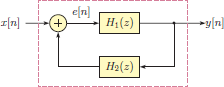
MATLAB Problems
8.48. The signal x[n] is given by
- Find X (z). Determine its poles and zeros. Manually construct a pole-zero diagram.
- Write a MATLAB script to evaluate the magnitude of X (z) at a grid of complex points in the z-plane. Use the function meshgrid(..) to generate the grid of complex points within the ranges −1.5 < Re {z} < 1.5 and − 1.5 < Im {z} < 1.5 with increments of 0.05 in each direction.
- Use the function mesh(..) to produce a three-dimensional mesh plot of |X (z)|.
- Evaluate the z-transform for z = ejΩ and use the function plot3(..) to plot it over the three-dimensional mesh plot.
-
Repeat Problem 8.48 with the signal
Repeat Problem 8.48 with the signal
8.50. Refer to the system in Problem 8.30.
Construct a system object for H (z) using the function zpk(..).
Compute the response of the system to the input signal
for n = 0,..., 49 using the function dlsim(..). Compare the first few samples of the response to the result of hand calculations in Problem 8.30.
8.51. Refer to the system in Problem 8.31.
- Write a MATLAB script to find the impulse response of the system by iteratively solving the difference equation found in Problem 8.31 part (c). Compute h[n] for n = 0,..., 10. Does it match the expected answer?
- Modify the script written in part (a) so that the unit-step response of the system is computed by iteratively solving the difference equation. Compare the result to that found in Problem 8.31 part (d).
- Construct a system object for H (z) using the function tf(..). Afterwards compute the impulse response and the unit-step response of the system using functions dimpulse(..) and dstep(..) respectively. Compare to the answers obtained in previous parts.
8.52. Refer to the DTLTI system in Problem 8.35.
- Write a MATLAB script to compute and graph the magnitude and the phase of the frequency spectrum for the system. Your script should also mark the points critical for the two input signals used in Problem 8.35.
- Graph the steady-state response to each of the two input signals specified.
8.53. Develop a script to compute the phase response of a first-order allpass filter with a real pole at p = r + j0 for parameter values r = 0.2, 0.4, 0.6, 0.8. Graph the four phase responses on the same coordinate system for comparison.
8.54. Develop a script to compute the phase response of a second-order allpass filter with a complex conjugate poles at
- In your script set θ = π/ 6 radians. Compute the phase response for r = 0.4, 0.6, 0.8, and graph the results superimposed for comparison.
- Set r = 0.8. Compute the phase response for θ = π/ 6, π/4, π/3 radians, and graph the results superimposed for comparison.
8.55. Refer to Problem 8.45.
- For each difference equation given, write a script to find the solution for sample indices n = 0,..., 10 using the iterative solution method with the specified initial conditions.
- For each difference equation given, write a script to find the analytical solution using symbolic mathematics capabilities of MATLAB.
MATLAB Project
8.56. In Problem 1.51 of Chapter 1 the generation of DTMF signals was explored using MATLAB's trigonometric functions. In this project we will explore alternative means to sinusoidal tone generation.
In some applications we may wish to use inexpensive processors that may either have no support for trigonometric functions or may be too slow in computing them. An alternative method of computing the samples of a sinusoidal signal is to use a discrete-time system the impulse response of which is sinusoidal, and to apply an impulse signal to its input. Recall that the z-transform of a discrete-time sine signal was found in Example 8.16 as
which could be used as the basis of a second-order system as shown in Fig. P.8.56(a). DTMF signals that correspond to digits on a keypad can be generated by using two systems of this type in parallel as shown in Fig. P.8.56(b) by adjusting the coefficients properly.
Develop a MATLAB function ss_dtmf2(..) to generate samples of the DTMF signal for a specified digit for a specified duration. The syntax of the function should be as follows:
x = ss_dtmf2 (digit,fs,n)The first argument “digit” is the digit for which the DTMF signal is to be generated. Let values digit = 0 through digit = 9 represent the corresponding keys on the keypad. Map the remaining two keys “*”and “#” to values digit = 10 and digit = 11 respectively. Finally, the value digit = 12 should represent a pause, that is, a silent period. The arguments “fs” and “n” are the sampling rate (in Hz) and the number of samples to be produced respectively. Internally you may want to use the function ss_iir2(..) that was developed in MATLAB Exercise 8.12.
Develop a function named ss_dtmf(..) with the syntax
x = ss_dtmf (number ,fs ,nd ,np)The arguments for the function ss_dtmf(..) are defined as follows:
number: The phone number to be dialed, entered as a vector. For example, to dial the number 555-1212, the vector “number” would be entered as
number = [5 ,5 ,5 ,1 ,2 ,1 ,2]fs: The sampling rate (in Hz) used in computing the amplitudes of the DTMF signal.
nd: Number of samples for each digit.
np: Number of samples for each pause between consecutive digits.
The function ss_dtmf(..) should use the function ss_dtmf2(..) to produce the signals for each digit (and the pauses between digits) and append them together to create the signal x[n].
- Write a script to test the function ss_dtmf(..) with the number 555-1212. Use a sampling rate of fs = 8000 Hz. The duration of each digit should be 200 milliseconds with 80 millisecond pauses between digits.
- Play back the resulting signal x[n]using the sound(..) function.
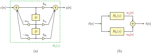
2 Remember that, for linearity, each subsystem must be initially relaxed. All initial values must be zero. In Fig. 8.50, for example, we need x [−1] = x [−2] = x [−3] = y [−1] = y [−2] = y [−3] = 0.