19.1 The introductory physics approach

The reader may be getting impatient to see some examples of real problems that can be solved without error, not just fiendishly clever challenges thought up by mathematicians. The behavior of a pendulum is one of the first dynamics problems introduced in any physics course, so start with that.

Unfortunately, it simply is not true. The restoring force is not proportional to the displacement. A pendulum is not a harmonic oscillator. Larger swings take longer than small ones, as anyone who has ever used a playground swing knows. Applying the wave equation to a pendulum is one of the “little lies” that sneak into the teaching of physics. The myth stems from the powerful desire to use the elegant analytical tools we have at our disposal and get results that look like elementary functions, even when … they do not quite fit the problem. A pendulum is approximately a harmonic oscillator the same way the earth is approximately flat, not round.

There is a theoretical solution for the true behavior of a pendulum, but it involves mathematics so ghastly that only a few undergraduate physics majors ever are exposed to it, and when you look at the “solution” it provides no insight into what is going on. There are many ways to express the exact description of pendulum motion, but all of them require combining an infinite number of elementary functions.

19.2 The usual numerical approach

Suppose that the pendulum swing starts with the pendulum held at an angle –60° from vertical, for a mass m on a string of length L.

The usual approach to simulating physical dynamics with a computer is to march through time steps, by performing the following steps repeatedly:

• Use the position to estimate the force on the mass.

• Use the force to estimate the acceleration.

• Use the acceleration and the present velocity to estimate the future velocity.

• Use the velocity to estimate the future position.

Each estimate is subject to sampling error because position, force, and velocity all vary within a time step. There are many sophisticated methods that try to be clever, say, by using an interpolation between past, present, and future accelerations and velocities to get closer to the truth, but they all commit sampling errors.

When performed with floating point numbers, the calculations accumulate rounding errors as well. Because of both sampling and rounding errors, the computed physics simulation drifts farther and farther from reality. And you have no idea how far the answer has drifted because all the errors are silent and invisible. Traditional numerical analysis also states the sampling error for time step methods with another deeply unsatisfying error bound like the ones for numerically computing the area under a curve. The amount of sampling error is written in terms of unknown quantities that could be infinite.

The ubox method is fundamentally different, and treats the time dimension simply as one more ubox dimension. Each ubox in the two-dimensional space of position and time must

• conserve energy,

• preserve continuity (no teleportation to a new point in space), and

• have no instantaneous changes in the velocity, since that would require an infinite amount of force.

Say the starting position is angle x = –60° as shown in the figure. Envision it as a child weighing 25 kilograms on a swing 2 meters long. Suppose for the moment that all values are exact, including the force of gravity as 9.8 meters per second squared.

The potential energy is mass m times gravity g times relative height h, or m g h. Here, the relative height is the distance to the bottom of the arc of the swing, which for a displacement angle θ is L (1 - cos(θ)). At the starting position, all the energy is potential energy because the velocity is zero. For this swing, the total energy is always 245 joules. (We can ignore air resistance, and assume someone is giving the child a slight push at the end of each cycle to keep the amplitude at ±60 °.)

Kinetic energy is 12my2, where v is velocity. It is the total energy minus the potential energy, since the total amount of energy is conserved.

That means velocity can be derived from the position. The velocity is in meters per second along the arc of motion, so the angular velocity in degrees must be scaled by ττL180o to find the velocity of the suspended mass M. The following formula infers the velocity from the kinetic energy; notice that this requires kinetic energy to be nonnegative, or else the velocity will be an imaginary number!

We can also determine the acceleration from the position. It is simply gravity times the negative sine of the deflection angle. (First-year physics approximates sin(θ) with θ to make things easier, albeit wrong.)

Problems like pendulum dynamics are called nonlinear ordinary differential equations. The convenient situation where position, velocity, and acceleration are related by simple linear equations does not happen nearly as often in real-world problems as it does in physics courses. Traditional numerical methods offer guesses about the solution to such nonlinear problems, but no guaranteed bounds for the answer to the simple question, “Where is the mass at any point in time?”

19.3 Space stepping: A new source of massive parallelism

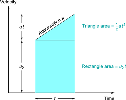
This diagram is a reminder that much of physics does not require calculus. Distance is velocity times time. If speed varies with time, then distance is the area under the function that describes the velocity. It does not take integral calculus to find the area if acceleration is constant; we only need elementary geometry for the area of a triangle and a rectangle.

Why not simply use χnew=χ01d+u0t+12 a t² with traditional interval arithmetic, using bounds on velocity u₀ and acceleration a to bound the value of x_new? Because doing so creates a chicken-and-egg problem: You do not know the range of possible accelerations and velocities until you know the range of possible positions in the time step. And you do not know the possible positions in the time step until you find out the range of possible accelerations and velocities. In the case of the pendulum, during the first quarter-period the velocity goes as low as zero and the acceleration also goes as low as zero, which means interval arithmetic predicts that the pendulum might not move at all, but just hang there having a Wile E. Coyote moment.

Instead, we treat time as a function of location. Within a location range, there is a rigorous bound on the velocity and the acceleration. (This happens for many types of dynamics problems, not just the pendulum.) From the bounds on velocity and acceleration, we can derive rigorous bounds on the time interval spent traversing each location range using elementary geometry, as we will show in a bit. This might make you uncomfortable because space stepping is backwards from the usual way we think about motion, where the location is a function of time. But consider this fact:

That is a stunning result, because it means we not only get rigorous bounds on the physical behavior, but we can use as many processors as we have in a computer system to get any desired answer quality. Nature may operate a pendulum as a serial function of time, but that does not mean we have to compute its behavior serially as well.

When people seek excuses not to use parallel computing to solve problems, they often point to problems that seem inherently serial, where things apparently have to be computed in sequential order (each step depends on the previous one). Pendulum simulation is a perfect example, and so is the problem of calculating an orbital trajectory. For many years, computer users have misused Amdahl’s law as an excuse not to apply parallel programming, asserting that doing so would have very limited benefit. Similarly, the time dependency of physical simulations has been misused as an excuse not to change existing serial software to run in parallel. It is now time to retire that excuse, also.

Each calculated traversal time will be off by some number of ULPs, and when we line all the times up to create the graph of where the mass is at any range of time, the ULPs accumulate. The unum environment should be selected so that the accumulated ULP error is about the same size as the accumulated theoretical bound between the slowest and fastest time, which can be made as small as we like by using more space steps. This is very different from rounding error and sampling error; it eliminates both sources of error in the numerical calculation, replacing them with guaranteed bounds.

Here is a simple example of how to bound the amount of time spent in an angle range. Start with the entire range from the start time at –60° to the point where the°. (After that the behavior is symmetrical, so calculating a quarter-period suffices to calculate the entire period of the swing.) The angle subscripts denote physical values at particular angles, so a_{-60 °} means the acceleration when the pendulum is at –60°, for example:

The purple curve shows the correct velocity as a function of time. We do not know what that velocity function is, but we do know what its physical limits can be. The maximum it can be is if it increases with the maximum acceleration a_{-60 °} up to the time when it reaches the maximum velocity v₀°, which is the curve shown in red. Notice the red dot where the maximum acceleration changes; that will help with visualization when we use the velocity to find the location.

The minimum, shown in blue, would be if the velocity accelerated only enough to get it to the maximum. Why can it not be even lower than that, and perhaps curve up toward the right? Because the acceleration is decreasing in this angle range. It cannot curve up anywhere, since that would mean acceleration is increasing.

The corner where the top curve hits the maximum velocity is when time is equal to v₀° /a_-60 °. With that, we have the coordinates of every point needed to find the formula for the area under the red curve and under the blue curve, both of which represent the distance traveled. But remember, we are not computing the distance traveled. We know the distance traveled; what we do not know is the time it takes to go through that part of the pendulum swing.

Adding up the area of the triangle and the rectangle under the red curve gives the minimum time to traverse the angle range, since that is the maximum velocity.

Solving this equation for t_min tells us the following:

For this particular pendulum, t_min evaluates to 0.733896 … seconds as the minimum possible time, which is interesting because the harmonic oscillator model says the period is 0.709613 … seconds! We just proved that the usual model derived from calculus is false, and did it with elementary geometry and algebra.

Now for the lower bound, the blue curve, which tells us the maximum time to traverse the angle range since it is the slowest possible speed. This one is simpler because the distance traveled is simply the area of a triangle:

Solving this for t_max tells us this:

That gives an upper bound on the time of 0.94632 … seconds. If the ubox bounds in time and space are calculated with a {2, 3 } environment (at most eight bits of precision in the fraction), the bounded solution is still tight enough to exclude the first-year physics solution, shown in amber on the graph below.

The dot on the red curve corresponds to the dot on the velocity curve in the previous plot. It shows when the acceleration changes, which is hard to see otherwise because the curve is smooth there. The plot shows a cyan ubound at the start and one at the end, but information about the bounds on the acceleration and velocity mean we have parabolic trajectories bounding the time and position in between. Notice that the starting ubound is exact in both dimensions, because we know the time is exactly zero and the location is exactly –60° (though the angle is plotted as position on the arc of the swing).

The final ubound is exact in the position because we know the position is exactly zero, and inexact for time. The unum bounds for the two red acceleration-velocity pairs and the single blue acceleration-velocity pair yield a rigorous bound for the trajectory using finite-precision arithmetic.

You can guess what comes next: Split the space region in two. Evaluate the acceleration and velocity at –30°, a -30°, and “pin” the bounding regions and slopes to those values. The shape bounds get more interesting:

A glance at the graph shows that this is already a much tighter bound on the unknown purple velocity curve. Plus, two processors can calculate the bounds on the two time periods in parallel. For this new subdivision of angle space, the area bounds work out to the following:

• Time spent going from –60° to –30 °: 0.50486 … to 0.55291 … seconds.

• Time spent going from –30° to –0 °:0.24595 … to 0.25494 … seconds.

That makes the total time from –60° to 0° somewhere in the interval 0.7508… to 0.8079… seconds, which is almost four times as tight as the bound we computed before, 0.7338 … to 0.9463 … seconds:

The computation at the midpoint angle adds a new ubound at exactly –30°. With the general technique defined for computing changes in time, try bounding the pendulum time using space steps of 10° arcs. The graphs are so precise that we have to use thinner lines to make the minimum time distinguishable from the maximum time. The first-year physics answer is so far off that it is easy to distinguish.

The cyan ubox bounds are almost too small to see, but they are exact in the vertical dimension and have a tiny range in the horizontal dimension that accumulates from the leftmost ubox (where we know the starting time exactly) to the rightmost one. The range is the result of both unum ULP widths and the variation in the velocity in each position range. If we had used higher-precision unums to reduce ULP widths, the final time range would be 0.759494 … to 0.768758 … seconds, a width of about 0.009 seconds. Recall that we used a {2, 3 } unum environment, so the largest possible fraction is only 2³ = 8 bits. This causes an additional information loss at each step, so the resulting bound is between 0.773438 … to 0.753906 … seconds, a range of about 0.02 seconds. This indicates a good match between the space step discretization and the unum precision, since neither one is using “overkill” to get the answer more accurate. If we had used, say, a {2, 4 } unum environment that could have up to 2⁴ = 16 bits in the fraction, that would have merited decomposing the problem into more space steps, staying in balance.

With a total of only six independent space steps, we calculated the pendulum behavior to almost three decimals of accuracy and with a provable bound. Furthermore, the most complicated math we used was grade school algebra. Without deep human thought but with brute force computing, we can bound the solution to any desired accuracy. In other words, we just “solved” a nonlinear differential equation without using any calculus.

This shows why it may be time to overthrow a century of numerical analysis. The classical way of solving a dynamics problem is either to substitute a different problem that has a tidy-looking solution involving only elementary functions, or to perform an error-filled time-stepping simulation that cannot run in parallel and has no rigorous bound on the numerical guesses it makes.

By combining space stepping with uboxes and unum arithmetic, we can obtain a bound that can be as tight as we want and can be computed using as many processor cores as we have at our disposal.

19.4 It’s not just for pendulums

The approach works whenever the kinetic and potential energy of a mass depend only on its position along a known path, allowing us to compute the velocity and the force as a function of position in space instead of time. It can, for example, bound the solution for a true harmonic oscillator (like a mass on an ideal spring). Many simulations of electric circuits that compute current and voltage in time steps can be rewritten to compute the time from the change in the circuit state, again applying energy conservation.

The pendulum example shows the promise of a general technique, one worth building a set of tools for. The technique requires that the force on a mass, and its velocity, are determined by the position of the mass. That would cover, say, the motion of a ball rolling down a slide with a complicated shape. It would not apply to something like a rocket, which decreases its mass as it burns fuel. (The popular expression “It’s rocket science” stems from the challenge of solving equations where the physics depends on both the position and the history of the rocket.)

Here is a general type of dynamics problem: A mass moves from point x₁ to point x₂. Its velocity at x₁ is v₁; its velocity at x₂ is v₂, and between x₁ and x₂ the velocity never goes outside that range. Similarly, the acceleration is a₁ at point x₁ and a₂ and point x₂, and never goes outside that range. What range of time t is required for the mass to make the trip? Notice we do not require that v₁ ≤ v₂ or a₁ ≤ a₂.

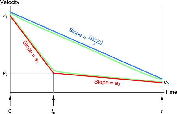
The graph on the next page indicates subtleties about velocity ranges when a₁ > a₂, with red indicating the maximum velocity and blue indicating the minimum velocity:

First, notice that the v₁ and v₂ are shown as inexact to remind us that they are computed values that will generally be represented with a ubound; that is, there is a gap between the red and blue lines at the left and right endpoints.

The first red slope is the upper bound of the calculated acceleration a₁ and the second red slope is the lower bound a₂. Actual physical behavior is mathematically bounded. Also, notice the two green curves. The bottom one starts out with a slope of a₁ as required, but almost immediately takes on a slope close to that of the line connecting the start and end points. Just before it gets to the end time t, it curves down just enough to match the slope of a₂, the acceleration at the end time. The lower bound shown as a blue line bounds the lowest possible velocity at any time. The upper green line takes on the higher acceleration a₁ for as long as it can, but at some time t_c it has to switch to acceleration a₂ or it cannot reach the final velocity v₂. Since instantaneous changes in velocity are impossible (it would take an infinite amount of force), the upper green line shows a rounded elbow at t_c.

The minimum travel time occurs when the velocity is maximum; the maximum time occurs when the velocity is minimum. The area under the blue line is the distance traveled, x = x₂ - x₁. If we were lazy, we could just say the minimum velocity is v₂ and the maximum velocity is v₁, so

The simple bound made it easy to invert the problem to solve for t as a function of x. The problem is that the minimum velocity could be zero, in which case the bound on the travel time is infinity, and that does not provide a useful answer.

The area under the blue line is easy to compute: x = χ=12(y1+y2)tmax, which inverts to tmax=2xv↑+v2. The area under the two red line segments is much more complicated, because we first have to find the point of intersection and the area is a second-degree polynomial in the time t, which means that inverting to solve for t requires solving a quadratic equation. Brace for algebra.

The two red lines intersect when

The area under the left red line segment is 12(y1+yC)tc and the area under the right red line segment is 12(yC+y2)(t-tc). After expanding those products and collecting terms, we get the total area:

Solving for t gives the minimum time, a complicated expression but nothing a computer cannot handle. With expressions for t_min and t_max, we can directly compute the range of possible times:

The minimum can also be computed using the solveforub function described in the previous chapter instead of using the quadratic equation, if a tightest-possible bound is needed. The situation is different if a₁ < a₂:

In this case, the equations for t_min and t_max are interchanged and we need the other ± case of the quadratic formula. We also need to handle the case where a₁ or a₂ is zero, and the trivial case where both are zero (that is, velocity is constant).

The implementation function delt below derives elapsed time from acceleration bounds, velocity bounds, and distance and is careful to account for the cases where either acceleration is zero. It was used to produce the preceding plots and is shown below. Its arguments are the acceleration bounds a1 and a2, the velocity bounds v1 and v2, and the distance to be traversed, x. A unum version of delt was used to do the ubox calculations of the pendulum behavior.

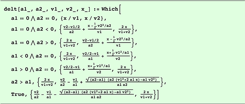
If our computer resources involve processors that can work in parallel, delt is the task that each processor can perform independently to solve this type of space-stepping problem. The only limit to the parallelism is how much precision is justified in the final answer. For instance, if we only know g = 9.80 to three decimals, it makes little sense to compute pendulum behavior to ten decimals of accuracy. The value of g ranges from 9.78036 at the equator to 9.83208 at the poles, and it also varies with altitude. If you use the following formula for g in meters per second squared, where p is the latitude and h is the altitude in kilometers, and the pendulum has little air resistance, then you might be justified calculating to seven decimals:

The adding of the times to reach any desired accumulated time can be done in parallel with a reduction operation like a binary tree sum collapse. Summing n values takes log₂ (n) passes with that method, a big improvement over doing it on one processor in n steps. Besides parallel summation being fast, the availability of a fused sum means there is no difference in the answer no matter how the time intervals are added.

With just a little added complexity to the sum collapse, the prefix sum can be calculated in about the same time, producing the partial sums t₁, t₁ + t₂, t₁ + t₂ + t₃, as well as complete sum. That restores the space-parallel answer to the usual way we think about simulations: Position (or some other quantity) as a function of time.

This chapter started with the sinusoidal plot of the classical solution to the pendulum problem. Here is the plot again, along with a plot of the rigorous ubox time bounds for the coarse 10º angle spacing. It may initially look like a small difference between the two results in the horizontal (time) dimension, but look at the difference in the displacement value for times toward the right part of the graph. For instance, when the pendulum is actually passing through 0º for the fourth time, the classical sinusoidal solution shows the pendulum around –40º, a huge error.

Since the uncertainty in the ubox method accumulates as the ranges of elapsed time accumulate from left to right, it is possible to see the spread of minimum time (red) and maximum time (blue). Decreasing the space step to 116 º not only makes the spread too small to show on the graph, it also fills in all the gaps in the plot. Since the maximum time is plotted after the minimum time, the blue plot covers the red plot.

What are the limits of applying ubounds and space-stepping to numerical physics? The chapters that follow show that the technique is certainly not limited to nonlinear ordinary differential equations.