D.1 ULP manipulation functions

To manipulate multidimensional ubounds (that is, uboxes), we need support functions that promote and demote the fraction size and exponent size. These must be used with care since they affect the ULP size, but they are useful when we can determine which end of the ULP-wide interval moves and which end stays put. Since the first two routines require exact unums as input, nothing will happen to the value they represent; they simply decompress the fraction field or exponent field by one bit. The reason it is more complicated to promote the exponent field is because subnormals behave differently from normals, and there is also the possibility that exponent promotion causes a subnormal to be expressible as a normal.

With floats, addition and subtraction are done by first lining up the binary point. An analogous operation is useful with unums, where two exact unums with different utag contents are promoted such that they both have the same exponent size and fraction size, using the previous two routines. That makes it easy to compare bit strings.

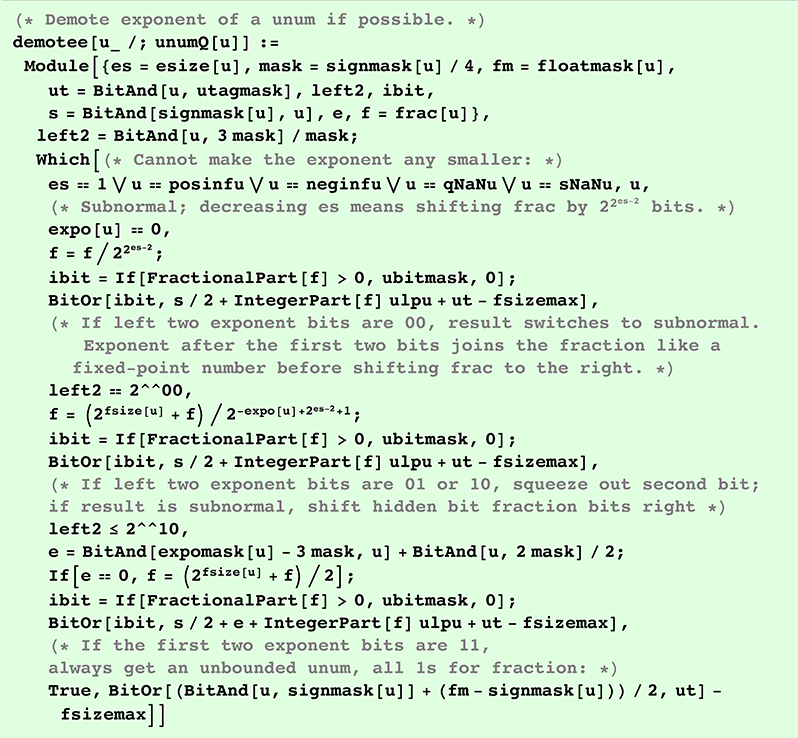
Some ubox routines need to intentionally coarsen a result. Demoting (reducing the length of) the bit fields for fraction or exponent can easily turn an exact unum into an inexact one, but it will remain a valid bound for the original value. The more complex field demotion routine is the one for the exponent, demotee:

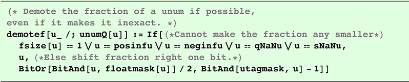
By comparison, fraction demotion (demotef) is very simple:

D.2 Neighbor-finding functions

Before finding neighbors on either side of a unum, we need three support functions The ulphi function finds the width of the ULP just to its right of an exact unum, taking into account its sign:

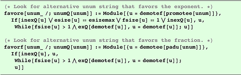
The favore and favorf helper functions prevent confusion stemming from unums that have more than one legitimate (shortest bit string) form.

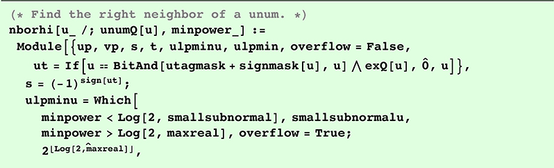
The nborhi function is surprisingly complicated, mainly because it allows a preferred minimum ULP size. If it were not for that, an unwanted level of detail might ensue, say, when crossing zero. In future versions, it should be possible to express preferred ULP sizes as relative widths, not just absolute widths. The following version suffices for the examples in this text. (Continues on next page.)

Fortunately, the only thing that has to be done to create the counterpart function nborlo is to negate the argument, use nborhi, and negate again. The real number line is conveniently symmetrical. Unfortunately, “negative zero” introduces a tiny asymmetry in the logic, so that exception is handled here:

The findnbors routine works in any number of dimensions to find all the nearest neighbor unums in the dimensions of a ubox set, using preferred minimum ULP sizes customized to each dimension from the minpowers list:

D.3 Ubox creation by splitting

The easiest way to create a list of one-dimensional uboxes that tile a range is to use uboxlist, which accepts a ubound and a preferred minimum ULP width expressed as an integer, the log base 2 of the preferred width. They will be larger than this request if the minimum ULP size is larger than the request, and they will be smaller near any endpoint that does not fall on an even boundary of 2^minpower.

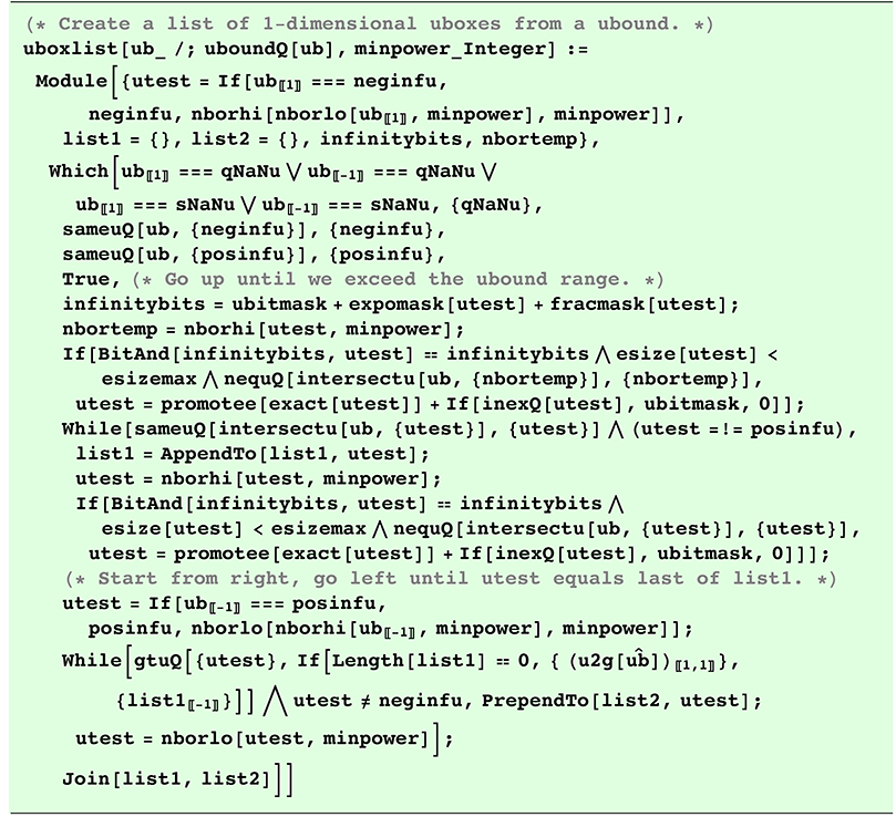
For some purposes (like the display of pixels on a screen), we can leave out the unums that are zero in any dimension. The uboxlistinexact routine is like uboxlist, but only produces unums that have nonzero width.

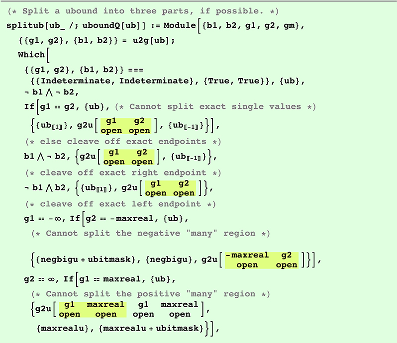
The next two routines are so similar that they probably should be consolidated. They both seek to split a range of values into smaller values representable in the u-layer, with a preference for the coarsest ULP resolution. The splitub routine prioritizes splitting off exact endpoints, so that repeated calls to it will eventually be given open intervals larger than an ULP. It then prioritizes the coarsest-possible ULP.

The bisect routine is a g-layer function that checks for infinite endpoint values, but for finite-valued endpoints it looks for the coarsest-possible integer power of 2 near the mean value.

D.4 Coalescing ubox sets

There are several ways to put sets of uboxes back together, and the prototype has a few primitive approaches for doing this in one and two dimensions. They are the most in need of algorithmic efficiency improvement of any of the routines here, since they are doing things in an order n² way that could be done in order n time. They also need to be more robust in handling overlapping uboxes. For example, the following pair of uboxes would not be coalesced.

The coalescepass routine examines a set for the occurrence of adjacent inexact-exact-inexact unum triples, since those can sometimes be replaced by a single inexact unum of twice the ULP width.

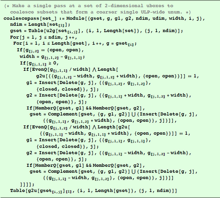
The coalesce routine (it really should be called coalesce2D) calls coalescepass until no more consolidation is possible.

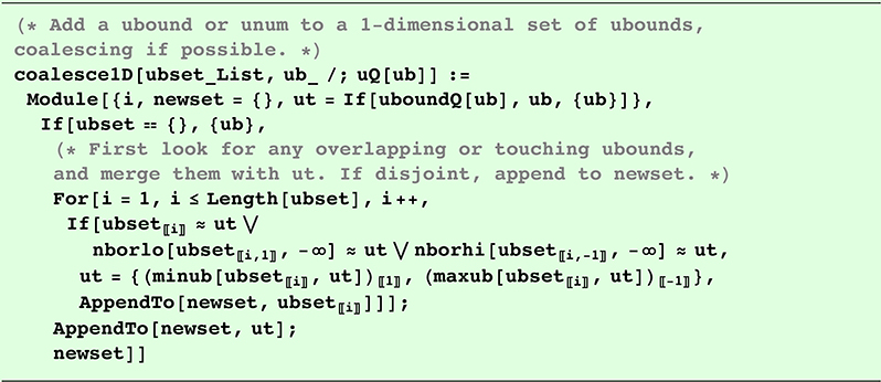
The next two routines are for one-dimensional ubox sets. The coalesce1D routine makes fewer assumptions about an existing ubox list ubset, attempting to merge an input argument ubound ub with that set if its ranges overlap or touch.

The ubinsert routine works in conjunction with the try-everything approach, and works very well when it starts out empty and can preserve ordering with each new candidate to add to the solution set. The commented Print statements can be un-commented to produce a monitoring of the progress of the solution-finding algorithm.

The hollowout routine is a little like consolidation; it removes interior points and leaves only the boundary. Sometimes that can be the most efficient way to operate with a multidimensional shape.

D.5 Ubox bounds, width, volumes

The minub and maxub functions find the leftmost and rightmost points on the real number line described by two ubounds, taking into account their open-closed states to break ties and to record the result.

The width and volume routines do just what they sound like they should do, with width returning the (real-valued) width of a unum or ubound, and volume returning the total multidimensional volume of a set of uboxes (following page):

D.6 Test operations on sets

The setintersectQ function has other uses, though; it tests if a ubound ub inter-sects any ubound in a set of ubounds, set:

The gsetintersectQ test does the equivalent for general intervals instead of ubounds:

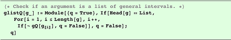
For safe programming practice, a function requiring a set of general intervals can be checked with glistQ to make sure every member of the set is a general interval.

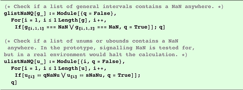
Since all it takes is one NaN to make an entire calculation a NaN, glistNaNQ can be called to return True if any entry is a NaN, otherwise False. The ulistNaNQ does the equivalent test for u-layer values.

The ulistQ test returns True if every member of the set is a unum or ubound.

D.7 Fused polynomial evaluation and acceleration formula

The routines for loss-free evaluation of polynomials use several support functions. The polyTg function uses a finite Taylor expansion to relocate the argument from powers of x (as a general interval) to powers of (x- x₀):

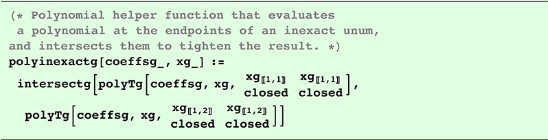
The polyinexactg function evaluates a polynomial using each endpoint as an x₀ in the polyTg function. The correct answer lies in the intersection of the resulting general interval; if this intersection is between the values of the polynomial evaluated at the exact endpoints, then there is no need for further refinement.

The polyexactg function takes an exact general interval xg and evaluates it exactly in the g-layer, using Horner’s rule. A fused multiply-add would work as the loop kernel also, but since the routine takes place entirely in the g-layer, there is no difference between fused operations and separate ones.

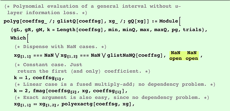
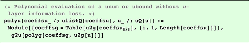
The polyg routine evaluates the polynomial of a general interval xg, using a set of general interval coefficients coeffsg (one for each power of xg from 0 to n), without information loss at the u-layer level of accuracy. The technique here should work for functions other than polynomials, if the equivalent of a polyTg function can be derived. (Continues to following page.)

The polyu function is the u-layer version of polyg. Unlike most u-layer functions, it does not tally the numbers and bits moved since its iterative nature makes it difficult to compare to a conventional polynomial evaluation. It clearly does more operations than the naïve method of evaluating the polynomial of an interval, but it is worth it to produce a result that completely eliminates the dependency error.

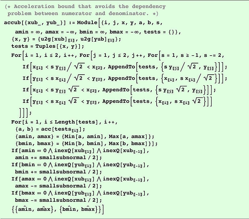
The accub function is shown here as an example of how to craft library functions that eliminate dependency error by fusing the operations. It was used in the chapter on gravitational dynamics. Because x and y appear in both the numerator and denominator of the formula for the acceleration,

there is some information loss when x and y are inexact. While numerical calculus is “considered evil” in Chapter 21, symbolic calculus is incredibly useful for finding the minima and maxima of functions in library function design. We can evaluate functions of inexact values by evaluating them at their endpoints and at any local extrema that lie within their range of uncertainty. By differentiating the acc function above with respect to x and y, we discover extrema along the lines y = ±2 x and x = ±2 y. So if we have a two-dimensional ubox for x and y, it always suffices to calculate acc at its corners and at any points in the range that intersect the lines y = ±2 x and x = ±2 y.

D.8 The try-everything solver

The solveforub [domain ] solver requires a conditionQ[ub] Boolean function to be defined by the user. Since it takes some practice to get the question right (see Chapter 17 for examples), the following code has some debugging-style Print statements that have been commented out. They can be un-commented to help discover why a routine is running too slowly or producing trivial-looking results because the wrong question was asked by conditionQ. A better version of solveforub would include a minpower parameter that prevents the solver from examining the real number line below a certain ULP size of 2^minpower, similar to nborhi and uboxlist. The function below will go to the limits of the settings of setenv, and will produce the c-solution for an initial search space of domain, where domain is a list of ubounds. In the worst case, it will iterate as many times as there are representable values in the environment, so it is best to set the environment low initially.

D.9 The guess function

As described in Chapter 18, the guessu [x ] function turns a unum, ubound, or general interval into an exact value that is as close as possible to the mean of its endpoints. When there is a tie between possible values that are as close as possible, the routine selects the one with the shorter unum bit string, which is the equivalent of “rounding to nearest even” for floats. This enables unums and ubounds to duplicate any algorithms that are known to be successful with floats, such as Gaussian elimi-nation and stable fixed-point methods. If the guess is to satisfy a condition, the guess can be checked by testing the condition using exact unum arithmetic. If it passes, then it is a provable solution, but there is no guarantee that it is a complete solution of all possible values that satisfy the condition. If the solution set is known to be connected, then the paint bucket method of Chapter 15 can be used to find a c-solution, using the guess as a seed.