
![]()
Testing of Hypothesis
You should now have an understanding of the basics of SAS and the fundamentals of statistics. You’ve mostly used descriptive statistics to explain the data and get some quick insights without applying any advanced techniques. One advanced technique you’ll learn to apply in this chapter is how to test your hypotheses. Learning how to test a hypothesis is important for analysts because they will use the process in many situations, such as when testing correlation, testing regression coefficients, testing parameter estimates in time-series analysis, testing the goodness of fit in logistic regression, and so on. You’ll learn about those topics in the coming chapters.
In this chapter, the focus is on testing of hypothesis and the important concepts involved in doing so. Specifically, you will learn about the null hypothesis, the alternate hypothesis, the process of testing a hypothesis, different types of tests to use, and finally the possibility of errors in the overall testing process.
Testing: An Analogy from Everyday Life
Let’s use a simple real-life example to conduct a test. Say you want to buy a 50-pound cake for a big party. You walk into a cake shop and ask for one. The store manager says it’s ready, and she shows it to you. You might get suspicious about its taste and quality. Fifty pounds is a giant cake, and obviously you don’t want to take any risks, even if the store manager assures you that it’s the best quality. In fact, you may want to test the cake. In other words, you would like to test the statement made by the store manager that the cake is of good quality. Obviously, you can’t eat the whole cake and claim you are just testing. So, you will ask the manager to cut a small piece out of the cake give it to you for testing. You might want to cut this test sample randomly from the cake. The following are the possibilities that might result from your test:
- The test piece is awesome and tastes like the best cake you have ever had. It may be an instant buy decision.
- The test piece is contradictory to your expectations. You will definitely not buy it in that case.
- The quality is not the best, but it is still satisfactory. You may want to buy it if nothing better is available.
You had an assumption to begin with, you then took a sample to test it, and you made a conclusion based on a simple test. In statistical terms, you made an inference on the whole population based on testing a random sample. This process was the essence of the testing of hypothesis, in other words, the science of confirmatory data analysis.
Let’s consider one more example. A giant e-commerce company claims that half of its customers are male and another half female. To test this statement, you take a random sample of 100 customers and count how many of them are male. Again, the following three scenarios may arise:
- Exactly 50 percent are males, and the other 50 percent are females.
- One gender dominates. For example, almost 90 percent are males, and only 10 percent are females.
- One gender is near 50 percent. For example, 52 percent are males in the sample.
In the first scenario, you agree to the statement made by the e-commerce company that the count of male and female customers is the same. In the second scenario, you simply reject the company’s claim. In the third scenario, you may tend to agree with the claim. Once again, you are making an inference on the whole population based on the sample measures.
These are reasonably good examples of the process of testing a hypothesis. It is summarized as follows:
- You start with an assumption.
- a. The whole cake is good in the first example.
- b. Overall, the gender ratio is 50 percent in the second example.
- You take a sample that represents the population.
- c. You try a piece of cake in the first example.
- d. You look at 100 customers in the second example.
- You do some kind of test on the sample gathered in step 2.
- e. You test the piece of cake by putting it in your mouth.
- f. You actually count the number of male and female customers in the sample.
- You make a final interpretation and inference based on the testing of random samples.
- g. You make a decision about whether the cake is good or bad.
- h. You make an inference about whether the gender ratio is really 50 percent or not.
What Is the Process of Testing a Hypothesis?
Testing a hypothesis is a process similar to the examples discussed in the previous section. Using this process you make inferences about the overall population by conducting some statistical tests on a sample. You are making statistical inferences on the population parameter using some test statistic values from the sample. You can refer to Chapter 5 for more about population, parameters, samples, and statistics, but here is a quick recap (see also Figure 8-1):
- Population: Population is the totality, the complete list of observations, or the complete data about the subject under study. Examples are all the credit card users or all the employees of a company.
- Sample: A sample is a subset of a population or a small portion collected from a population. Examples are credit card users between 20 and 30 years old and employees who are part of the HR team.
- Parameter: Any measure that is calculated on the population is a parameter. Examples are the average income of all credit card users and the average income of all the employees in your company.
- Statistic: Any measure that is calculated on the sample is a statistic. Examples are the average income of a sample from credit card users (users between 20 and 30 years old) and the average income of HR team employees.

Figure 8-1. Parameter and statistic
In inferential statistics, you make an assumption about the population. That assumption is called the hypothesis (the null hypothesis to be precise). You take a sample and calculate a test statistic, and you expect this test statistic to fall within certain limits if the null hypothesis is true.
Table 8-1 contains a few more examples involving the process of testing a hypothesis.
Table 8-1. Examples of Testing a Hypothesis

Up to now, we’ve talked about framing the null hypotheses, taking a random sample, sampling the distribution, calculating the probability, and finally making an inference on the population. Figure 8-2 illustrates the main steps involved in the process of testing a hypothesis.

Figure 8-2. An overview of steps involved when testing a hypothesis
Here are the steps again:
- State the null hypothesis on the population. Start with an assumption or hypothesis.
- Select the sample and sampling distribution.
- Calculate the test statistic value.
- Make a final inference based on the test statistic results.
Here’s a short business case study to help you understand the process of testing a hypothesis. A soap production company claims that the average weight of soap is 250 grams, and the population has a standard deviation of 5 grams. You want to test this by taking a sample of 50 bars of soap. You need to note that the soaps are priced based on the assumption that they weigh 250 grams. Anything more than 250 grams is a loss to the company. If the average weight is significantly less than 250 grams, then the company loses its customers; if it is greater than 250 grams, then the company is pricing its soap too low. In this case study, you can test a hypothesis to verify that the average weight of the bars of soap is 250 grams. Imagine that you take a sample of 50 soap bars and the sample average weight is 260 grams. Now the question is, should you accept or reject the null hypothesis?
The flowchart in Figure 8-3 shows the approach of testing the example hypothesis.
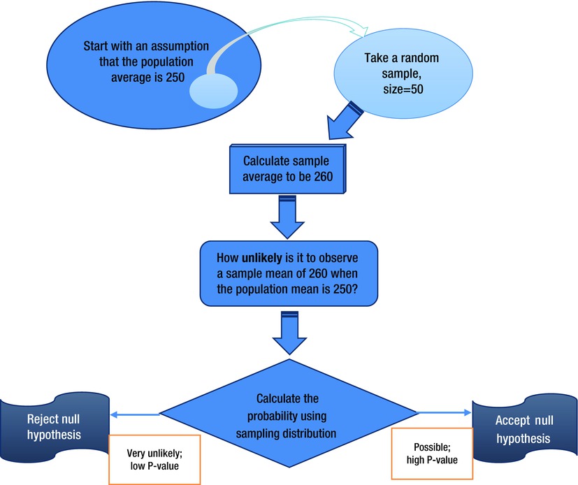
Figure 8-3. Testing a hypothesis for the soap example
Figure 8-4 shows all the steps involved in the process of test of hypothesis.

Figure 8-4. Establishing the null hypothesis, the first step
State the Null Hypothesis on the Population: Null Hypothesis (H0)
The null hypothesis is a statement or the initial assumption or claim about the overall population. A null hypothesis is generally denoted by H0 (pronounced “H not”). You need to be careful while stating the null hypothesis because you are going to perform the rest of the testing based on the assumption that the null hypothesis is true. In other words, you consider all the scenarios and measures based on the initial assumption of the null hypothesis. The null hypothesis is the simplest form of hypothesis. You will tend to agree all the statements in the null hypothesis unless you get some substantial evidence to not accept it.
The null hypothesis, H0, characterizes a theory, which is given either because it is thought to be true or because later it will be used as a basis for argument, but so far it has not been proved.
Here are some examples of null hypotheses:
- H0: Our customer base is 50 percent male.
- H0: The average height of the country’s female population is 5.5 feet.
- H0: Vaccination and flu are independent of each other.
- H0: The drug has no significant side effects.
- H0: This coin is unbiased or fair (the probability of heads equals the probability of tails, 0.5).
An alternative hypothesis is the second hypothesis that is a substitute to the null hypothesis. After the testing, if you are rejecting the null hypothesis, then you may consider accepting the alternative hypothesis. In most of the inferences (but not all), the alternative hypothesis is the opposite of the null hypothesis. Most of the time, you either accept or reject the null hypothesis, and the alternate hypothesis may not come into the picture at all. For ease of understanding, people use “rejecting the null hypothesis” as the same as “accepting the alternative hypothesis.” In short, you may not need alternative hypotheses for all types of tests. Alternate hypotheses for the examples in the previous section (for the null hypotheses) are shown here:
- H1: The percentage of male customers is not equal to 50 percent.
- H1: The average height of the country female population is not equal to 5.5 feet.
- H1: Vaccination and flu are dependent on each other.
- H1: The drug has significant side effects.
- H1: This coin is biased (the probability of heads and the probability of tails are not equal to 0.5).
The null and alternative hypotheses the soap example would be as follows:
- H0: The average weight of the soap is 250 grams.
- H1: The average weight of the soap is not equal to 250 grams.
Once you have defined the null hypothesis, you need to take a sample and calculate a statistic. Even before calculating the statistic, you should have a clear idea about what the distribution of the sample statistic will be. This is also known as the sampling distribution (Figure 8-5).
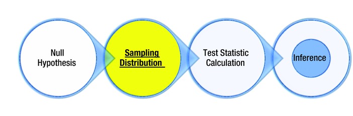
Figure 8-5. Sample distribution, the second step
A sampling distribution is the distribution of the statistic on simple random sampling with replacement (SRSWR). In the soap example, imagine there are a million bars of soap in the population. What will the sampling distribution of the average weight be when you take the average weight from multiple samples? You simply take a sample of 50 soaps and find the average weight; let’s say it’s 260 grams. What will the distribution of the values of the average weight be if you repeat this same sampling exercise?
![]() Note While dealing with multiple samples in SRSWR method, you take a sample and replace it in the population before taking any other sample.
Note While dealing with multiple samples in SRSWR method, you take a sample and replace it in the population before taking any other sample.
Figure 8-6 shows that the overall population size is 1,000,000 and the overall average is 250 grams. Now you take a random sample of 50 soaps, find the average weight, and replace them in the population. You take another random sample of 50 soaps and again calculate the average weight. If you repeat this process of simple random sampling with replacement and find the average weight for each sample, what will the distribution of weights be? Read on to get the answers!
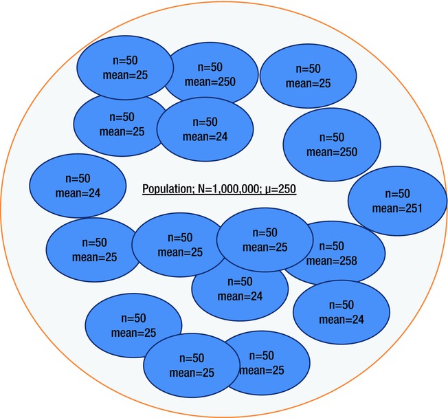
Figure 8-6. Multiple random samples in the soap example
If you repeat this sampling infinite times and find the average weight of each sample, the probability distribution of average weight is called the sampling distribution. Figure 8-7 shows an imaginary frequency distribution for this example, when you take 3,000 simple random samples with replacement. From this frequency distribution, you can get an idea of how the probability distribution will look. The probability distribution, as discussed earlier, will require an infinite number of samples to be taken.

Figure 8-7. Frequency distribution of the sample mean in the soap example
Figure 8-7 probably answers all of the previous questions. Your understanding will further develop as you read about the central limit theorem in the following section.
You can see from the frequency distribution that for most of the samples you get a sample mean of 250 or a value near to it. Rarely you get a sample with a high deviation from the overall population mean.
The example discussed in Figure 8-7 is still not sufficient for you to get an understanding of the exact sampling distribution (the probability distribution of sample mean) of a sample mean. A frequency distribution of 3,000 test cases is not sufficient; you want to get the sampling distribution when you infinitely repeat the process of simple random sampling with replacement. The central limit theorem, discussed next, helps you in understanding the distribution of the sample mean.
To understand the philosophy behind the process of testing a hypothesis, you need to understand the central limit theorem. The following statement is a simplified form of the central limit theorem:
The distribution of the means of large samples tends to be normal, regardless of the distribution of the parent population.
We’ll now elaborate on this theorem. Imagine that a large number of random observations are taken from a population and an arithmetic mean of these observed values is computed. If you repeat this procedure a number of times and get a large number of such computed arithmetic means, the central limit theorem states that these computed means will be distributed as per an approximate normal distribution (the bell curve), regardless of the distribution of the underlying parent population.
The central limit theorem has three subtheorems:
- The mean of the sample means distribution is always equal to the mean of the parent population.

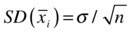
- The standard deviation of the sample means distribution is always equal to the standard deviation of the parent population divided by the square root of the sample size.
- The distribution of the sample means will increasingly approximate a normal distribution as the size, n, of samples increases.
Use of Central Limit Theorem When Testing a Hypothesis
You use the central limit theorem to test whether the population mean is equal to μ (the population arithmetic mean). To test the population mean, you take the sample mean, ![]() . The central limit theorem states that the sample mean follows the normal distribution. You try to quantify the probability of getting a sample mean of
. The central limit theorem states that the sample mean follows the normal distribution. You try to quantify the probability of getting a sample mean of ![]() or more. If that probability is much less, then you reject the null hypothesis.
or more. If that probability is much less, then you reject the null hypothesis.
In Figure 8-8, you can see the sample distribution of the mean values of the samples.
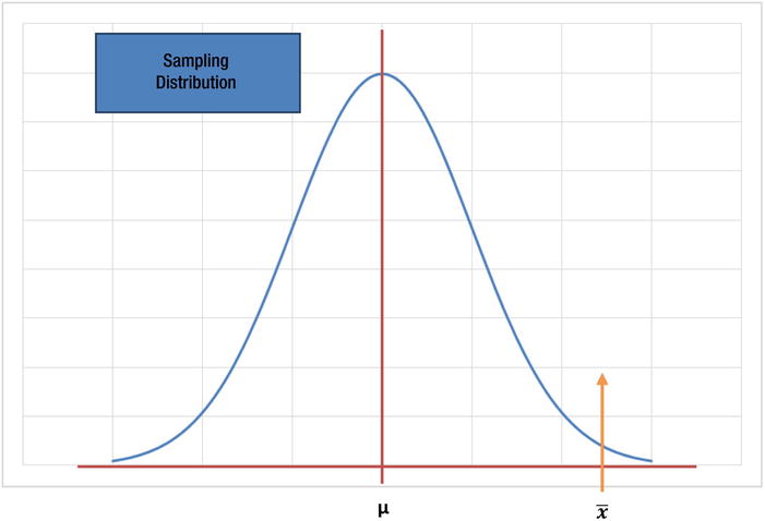
Figure 8-8. Sample distribution of the mean values of the samples
The mean of the sample means distribution is same as the population mean; it’s in accordance with the central limit theorem. Here you try to find the probability of getting a sample mean of ![]() or more if it is really taken from a population of mean μ. You accept or reject the null hypothesis based on the resultant probability. If the resultant probability is much less, then you reject the null hypothesis. Here, you are basically trying to test whether the sample is really coming from a population of mean μ.
or more if it is really taken from a population of mean μ. You accept or reject the null hypothesis based on the resultant probability. If the resultant probability is much less, then you reject the null hypothesis. Here, you are basically trying to test whether the sample is really coming from a population of mean μ.
In simple terms, if your calculations show that the probability of getting a specific value of sample mean (or worse) is much less and you still get that value of mean from your sample, then something is fishy. It simply means, with a reasonably accuracy, that the sample is not coming from the population for which it is claimed. In the soap example, the population mean is claimed to be 250 grams, and the sample mean is 260. Now you calculate the probability of getting a sample mean of 260 (or more) when the sample is taken from a population of mean 250. If this probability is much less (less than a predetermined threshold value), then with a reasonable confidence you can reject the null hypothesis that the population mean is 250.
Sampling distribution of the mean values of samples follows normal distribution. The sample mean follows normal distribution, but you can’t use the same theorem for all sample statistics. Sample variance doesn’t follow normal distribution. If the sample size is less than 30, then the sampling distribution is not normal. Table 8-2 contains some more examples of hypotheses, samples, and their corresponding distributions.
Table 8-2. Examples: Samples and Their Corresponding Distributions

In the soap example, you are also testing the population mean only, so you can apply the central limit theorem. The sampling distribution for the soap example looks like Figure 8-9.

Figure 8-9. Sampling distribution for soap example
Now you need to decide whether a sample mean value of 260 is far or near to the population mean of 250. How far is really far? You need to answer the question, how likely is it to get a 260 sample mean when the sample is taken from a parent population of mean 250? You need to measure the probability of getting a sample mean of 260 or more when its parent population has a mean of 250. You need to calculate and transform the statistic to find the probability and then accept or reject the hypothesis.
A test statistic (Figure 8-10) is the measure that is calculated from the sample. Sometimes the sample statistic alone might not be directly useful for finding the probability, but you can transform it and find the probability.

Figure 8-10. Test statistic, the third step
The test statistic selection will depend on the assumed probability distribution and the null hypothesis. Most of the time, it’s simply the sample statistic value. In the soap example, the sample mean is the test statistic value. The sample mean follows the normal distribution. Sometimes, to find normal distribution probabilities, you need to transform normal distribution to a standard normal variate. Table 8-3 shows a few examples of test statistics. The test statistic here is chosen based upon the type of problem.
Table 8-3. Examples of Test Statistic

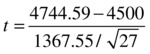
In the soap example, the test statistic is the mean value of the sample, that is, 260 grams. To find the probability, you transform it to the standard normal distribution. Instead of calculating probabilities directly from the given sampling normal distribution, you are converting the statistic to the standard normal distribution. This way it is easy to calculate the probability, and standard normal probability tables are available in several documents and tools. ![]() follows the normal distribution with mean 250, and the population standard deviation is given as 5 grams. The following formula is the test statistic for the sample means (when the sample size is more than 30):
follows the normal distribution with mean 250, and the population standard deviation is given as 5 grams. The following formula is the test statistic for the sample means (when the sample size is more than 30):

The formula will use the following values:
 = 260 is the mean value of the sample.
 = 250 is the population mean, which is the null hypothesis
- S = 5 is the population standard deviation.
- N = 50 is the sample size.


![]()
Now that the test statistic is ready, you need to give your inference; that is, you need to accept or reject the null hypothesis.
Now you know the exact test statistic value. Is it near to the null hypothesis? Or is it far away from the null hypothesis parameter? You can accept or reject the null hypothesis based on this test statistic point and its distance from the null hypothesis parameter. The acceptance or rejection of hypothesis is called inference.
Inference
Inference is the last step in the process of testing a hypothesis (Figure 8-11).

Figure 8-11. Inference, the fourth step
In this step, you decide whether you should accept or reject the null hypothesis. You accept the null hypothesis if the test statistic is within the permissible limits. If it is beyond the permissible limits, then you reject it. You can decide by looking at the P-value, or the probability value.
The P-value is the most important measure when testing a hypothesis. As discussed, you consider a sample and then calculate a test statistic. For example, if you are testing the population mean and if the sample mean is far away from the hypothesized mean, you reject the null hypothesis. But how far is really far? If the null hypothesis says the mean is 250 and your sample gives a value of 260, is it really far from 250? Are you OK with 251 as a sample mean? Is 252 fine? What are the actual boundaries you should have? To decide these boundaries, you need to understand sampling distribution.
When testing the sample, you got a sample mean of 260. Now you can actually find the probability of getting a sample mean of 260 or more when the sample is coming from a population having a mean value of 250. This is called the P-value.
- The P-value tells you what the probability is of observing this current test statistic value, or worse, when the sample is coming from a population that is complying with the null hypothesis.
- Imagine that your null hypothesis is true (the population mean equals 250). You can’t expect every sample statistic (sample mean) to have the same value as the population parameter. It can be higher or lower than the population parameter. Fortunately, the P-value gives you the probability of such an event. For example, you are drawing a sample from a population that really has a mean of 250. Obviously, you can’t expect every sample to have exactly a 250 mean. By chance if you get a mean of 260, the P-value will tell you what the probability is of getting a sample mean of 260 or more when the sample is drawn from a population of mean 250.
- What is the probability of observing the current statistic or an extreme value? The P-value is the answer to this question.
- The P-value is the measure of likelihood of obtaining a test statistic (as much or more) when H0 is true.
Figure 8-12 illustrates the definition of a P-value.

Figure 8-12. P-value explained
In Figure 8-12, imagine the null hypothesis states that the population has a mean of μ and the observed sample mean is t. The P-value is the area under the probability curve from t and above P(x>=t). The probability can be easily calculated by getting help from the sampling distribution properties. Here is a summary of the P-value:
- You start with a null hypothesis.
- You take a sample and calculate a statistic to test the null hypothesis.
- If the null hypothesis is true, then the statistic is expected to follow certain probability distribution.
- If it follows a particular probability distribution, then you can find the probability of getting the test statistic or beyond. This is the P-value.
After understanding the P-value, it’s not too difficult to comprehend its practical applications. If the P-value is high, then t is very close to μ, which means you may accept the null hypothesis. If the P-value is low, then t is very far from μ, which means you may have to reject the null hypothesis. Generally 5 percent is taken as an industry standard for the P-value. If the P-value (the probability) is more than 5 percent, then the null hypothesis is accepted. For a P-value less than 5 percent, the null hypothesis is rejected. If the P-value is less than 5 percent, then the sample statistic, t, is said to be significantly different from the population parameter.
Figure 8-13 shows a high P-value of around 25 percent. The sample statistic is also seen close to the population parameter.

Figure 8-13. P-value close to 25 percent
The graph in Figure 8-14 shows a low P-value of around 1 percent.

Figure 8-14. P-value close to 1 percent
The sample statistic is far from the population parameter, which means the statistic value is significantly different from the population parameter. If the sample is really coming from the population of mean μ, it should not be significantly different. In other words, the sample value should be near μ, which is not the case, so you reject the null hypothesis.
In the soap example, you got a sample mean of 260, when the population mean is 250. To see the probability of getting a sample mean of 260 or more (P-value), you used a standard Z-value normal probability curve that gave you the P-value.
In the “Test Statistic” section earlier in this chapter, we had calculated the z value for this example.
![]()
Now, what is the probability of getting a Z-value greater than or equal to 14.14?
P(z>=14.14)=?
From the standard normal tables, you can find the previous probability value of Z>=14.14,
P(z>=14.14)=1.54*(10-44)
which means P(z>=14.14) < 0.000000000000000000000000000000001.
Figure 8-15 shows the P-value for the soap example.

Figure 8-15. P-value for the soap example
Generally, if the P-value is less than 5 percent, then you reject the null hypothesis. Here, the P-value is not only less than 0.05, it is even less than 0.0000000000000001. Hence, you reject the null hypothesis. Here is another way of looking at this P-value:
- The null hypothesis states that the population mean is 250. If the sample is coming from a population of mean 250, then its sample mean should be nearly 250. In this exercise, you found the probability of getting 260. The sample doesn’t seem to come from a parent population of mean 250. You got a sample mean of 260. The probability of such a chance is less than 0.000000000000001. Hence, you reject the null hypothesis. If it would have been greater than 5 percent (2.5 percent on either side), you would have accepted the null hypothesis.
- The null hypothesis states that the population mean is 250, and you got a sample mean of 260. How far is it from the hypothesized mean of 250? Given the P-value, it looks very far. If the sample statistic would have been near to the population parameter of 250, then the P-value should have been 20 percent, 25 percent, 30 percent, or at least 5 percent (the least acceptable value). But in this example, the P-value is less than 0.0000000000000001.
- Based on the P-value, you can conclude that the null hypothesis is not correct, and you should reject it. Let’s consider another example. What is the probability of a football team winning 144 matches (with equal opposition) successively? You see that it is nearly equal to getting a sample mean of 260 when it is coming from a population mean of 250. The following bullets quantify these two probabilities:
- Probability of a football team winning 144 consecutive matches = 4.48*(10-44)
- Probability of getting a sample mean of 260 when the population mean is 250 = 1.48*(10-44)
Both these probabilities are extremely low. In fact, both these events are almost impossible; hence, you reject the null hypothesis.
Critical Values and Critical Region
Critical values are the boundaries between the acceptance and rejection regions. The critical region is the rejection region beyond these values (Figure 8-16). You have a 5 percent probability region where you reject the null hypothesis that is the critical region. Before the start of test, you decide this critical region for 5 percent or 10 percent or 1 percent.
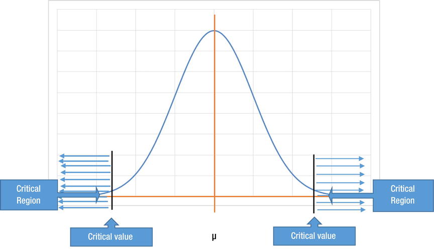
Figure 8-16. Critical value and critical region
If a test statistic value falls in the critical region, then the null hypothesis will be rejected.
A 5 percent tolerance means 2.5 percent on the either side of the null hypothesis value. Similarly, 10 percent means 5 percent on both sides, and so on. Generally, the P-value is sufficient to make a decision on accepting or rejecting the null hypothesis.
In the soap example, you got a Z-statistic value of 14.14. It falls within the rejection region or critical region. For a 5 percent critical region, on either side of null hypothesis mean, the critical values (based on standard normal probability tables) are -1.96 and 1.96 (Figure 8-17).
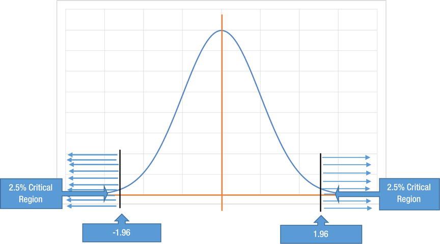
Figure 8-17. Critical value and critical region – the actual values
The test statistic value is in the critical region; it is beyond 1.96. Hence, the null hypothesis is rejected.
The confidence interval gives an estimate of the interval of values that a population parameter is likely to be in. The lower and upper limits of the confidence interval are called confidence limits. The confidence interval gives you an idea of the acceptable null hypothesis based on the test statistic. If you have fixed the level of significance as 5 percent (in other words, if 5 percent is the rejection region), the remaining 95 percent will be a nonrejection region. In that case, 95 percent will be calculated as the confidence interval.
You have to put the original null hypothesis aside for some time while dealing with confidence limits or the confidence interval, which is calculated solely based on the test statistic. It has nothing to do with the original null hypothesis.
In Figure 8-18, you can see the original distribution based on the null hypothesis (the solid line).

Figure 8-18. Confidence intervals
The dotted line shows a distribution based on the calculated sample statistic. The confidence interval in this example includes the null hypothesis. So, there is a higher chance to accept the null hypothesis.
If you get a test statistic of Z, then the confidence interval will be given by two limits of Z-l, and Z+l. The number l represents the confidence limits on both sides of Z. These are the two limits within which any null hypotheses will be accepted.
Let’s look at another example of working with confidence intervals. Say a health program in a preschool involves checking the weight of all the students. The school claims that the average weight of the students is 30 pounds. You need to test this claim and will use the following hypotheses:
- The null hypothesis: H0=30 (the average weight of students is 30 pounds)
- Alternative hypothesis H1≠30 (the average weight of students is not 30 pounds)
Since you don’t know the population standard deviation and you are testing the sample mean, you will use a T-test. (See Table 8-8 later in this chapter for more details.) The choice of test depends upon the null hypothesis and the sampling distribution of the test statistic.
We will explain the details of the SAS code and testing procedure later in the chapter. For now just consider the confidence interval for the output (Table 8-4).
Table 8-4. Confidence Interval for the School’s Health Check Data
|
Mean |
95% CL Mean | |
|---|---|---|
|
40.3796 |
38.9624 |
41.7967 |
Table 8-4 shows that the sample mean is 40.37. And the 95 percent confidence limits around the mean are 38.96 and 41.79. This mean is based on the sample statistic.
Figure 8-19 illustrates this scenario.

Figure 8-19. The population and sample mean values for school health check data
You can expect the population mean to be between 38.96 and 41.76 almost 95 percent of the time. If the null hypothesis is beyond these limits or beyond this interval, you can reject it. So, the null hypothesis of H0 = 30 will be rejected in this case.
Table 8-5 summarizes some facts about the process of testing a hypothesis. We are using the example discussed earlier about a company claiming that there are 50 percent males in its customer population.
Table 8-5. Summary of Facts for the Process of Testing a Hypothesis Using an Example
|
Sr No |
Testing of Hypothesis Facts |
Example Claim: 50 Percent Male Population in the Customer Base |
|---|---|---|
|
1 |
If the null hypothesis is true, then you expect the sample statistic to be within certain limits. |
If the overall population has a 50 percent gender ratio, then you expect the sample also to have a gender ratio of 50 percent. |
|
2 |
By chance if the sample statistic falls beyond the expected limits, then you calculate the probability of that chance or how likely that event is, called the P-value. |
If the proportion is not 50 percent in the sample and if you get, say, 70 percent males by chance in the sample, then you use sampling distribution to calculate the probability of observing 70 percent or worse. |
|
3 |
If it is very unlikely to witness what you observed in the sample, then you reject the null hypothesis or if the probability of that rare event is less than a predefined threshold value, then you reject the null hypothesis. |
If you have a sample with a 70 percent male population (the event) when the sample is taken from a population where there are 50 percent male and if you see that the probability of such an event is extremely low or lower than 5 percent, then you reject the null hypothesis. |
Tests
The type of test depends upon the sample statistic and the distribution of the sample statistic. If your sample statistic is a sample mean for a large sample, then you use a Z-test. If you are dealing with the sample mean of a small sample or if you don’t know the standard deviation of the population, then you use a T-test. Let’s look at a T-test for mean and some other example tests.
You use a T-test for the mean to test the null hypothesis, which may be something like the mean of a population being equal to a certain value. You use a T-test when the sample size is small. When the sample size is large, the sampling distribution is normal. But when the sample size is small, then the sample mean does not follow a normal distribution. The sample mean for small samples (less than 30) follows T-distribution with n-1 degrees of freedom (where n is the sample size). The T-distribution is similar to a normal distribution. As the sample size increases, the T-distribution tends toward a normal distribution. You use a T-test when the sample size is small or when the population standard deviation is not available.
![]() Note Degree of freedom, in simple terms, is the number of observations that can be chosen independently to form one particular T-distribution. You will further deal with degree of freedom in the following case study. The test statistic for a T-test is also the same as the test statistic for the Z-test, except that you don’t know this standard deviation of the population in a T-test.
Note Degree of freedom, in simple terms, is the number of observations that can be chosen independently to form one particular T-distribution. You will further deal with degree of freedom in the following case study. The test statistic for a T-test is also the same as the test statistic for the Z-test, except that you don’t know this standard deviation of the population in a T-test.

Let’s look at a brief case study to apply the concepts discussed so far.
Case Study: Testing for the Mean in SAS
Imagine a business scenario in which the city marketing manager of a smart TV company wants to devise a marketing strategy for its new TV model. She wants to have an effective strategy to reach the customers. For this, she needs to get an idea of the average monthly expenses of customer households in her city. An average estimate of expenses given by a local market research company is $4,500. The manager is not really confident about the accuracy of this figure. She wants to validate this figure before using it to devise her marketing strategy. She advises one of her teammates to collect some sample data on the expenses of a few randomly chosen families. Table 8-6 contains the sample data for 27 families.
Table 8-6. Monthly Expense Data for a Sample of Households
|
Sr No |
Expense |
|---|---|
|
1 |
4650 |
|
2 |
4248 |
|
3 |
4961 |
|
4 |
3200 |
|
5 |
4438 |
|
6 |
4993 |
|
7 |
4620 |
|
8 |
1100 |
|
9 |
4237 |
|
10 |
4991 |
|
11 |
4533 |
|
12 |
4457 |
|
13 |
4663 |
|
14 |
4613 |
|
15 |
4484 |
|
16 |
4997 |
|
17 |
5027 |
|
18 |
4807 |
|
19 |
4435 |
|
20 |
4503 |
|
21 |
9000 |
|
22 |
3950 |
|
23 |
4972 |
|
24 |
4983 |
|
25 |
8300 |
|
26 |
4516 |
|
27 |
4426 |
You are trying to test whether the population really has $4,500 as their average monthly expenses. You are testing the population mean, and the sample size is small, so you use a T-test. Here are the steps that you follow:
- State the null hypothesis.
The null hypothesis (H0): The average expense is equal to $4,500.
The alternative hypothesis (H1): The average expense is not equal to $4,500.
- Decide the sampling distribution and level of significance.
You are testing the sample mean for a small sample; hence, you will use T-distribution. And the level of significance is the same as the industry standard, in other words, 5 percent. So, the sampling distribution is a T-distribution with 26 degrees of freedom. T-distribution is not the same for all types of sample sizes. The T-distribution needs to be mentioned along with the degrees of freedom, which are equal to the sample size-1 (n-1). To reiterate, degree of freedom for a T-distribution is the number of observations that can be chosen independently to form one particular T-distribution.
- Test the statistic.

- Make an inference.
To make an inference on the overall population, you need to calculate the P-value using T-distribution with 26 degrees of freedom.
P = Probability of (t>0.93)
You can use distribution tables or a T-distribution probability value in any tool to get the previously mentioned probability. The value of P is as follows:
P = 0.361
The final inference is that the P-value is much more than 0.05; hence, you don’t have much evidence to reject the null hypothesis. You agree with the null hypothesis, in other words, that the value of the average expenses given by the market research team is correct or that there is not much evidence to prove that the values given by the market research team are wrong.
You can also use the following SAS code to perform the same test:
proc ttest data =Expenses H0 = 4500;
var expense;
run;
- The H0 option in the SAS code refers to the population hypothesized mean.
- The variable name in the data set is expense.
- The data set name is Expenses.
Table 8-7 shows the output of this code.
Table 8-7. Output of proc ttest (Data =Expenses)(the T-test Procedure; Variable: expense)

The output gives the sample size, sample mean, sample standard deviation, and minimum and maximum values of the variable expenses.
The third table in Table 8-7 is the most important one for the inference. It shows the T-statistic value. The T-statistic value is calculated from the test statistic equation. The P-value of the previous test is 0.3613. Based on the P-value, you accept the null hypothesis.
In the second table of the output tables in in Table 8-7, 95 percent confidence limits for the mean are given. The interval (4203.6 to 5285.6) has a 95 percent chance to contain the population mean.
Other Test Examples
Table 8-8 contains examples of other types of tests, including a Z-test, Chi-square test, and more.
Table 8-8. Some More Test Examples
|
Scenario |
Null Hypothesis |
Test |
|---|---|---|
|
Testing sample mean with large sample |
Population mean = X1. |
Z-test |
|
Testing sample mean with small sample |
Population mean = X2. |
T-test |
|
Testing the independence of two variables |
The two variables are independent. |
Chi-square test |
|
Testing correlation between two variables |
Correlation The correlation between two variables is zero. |
Person correlation test |
|
Testing the significance of an independent variable on a dependent variable |
Coefficient The coefficient of independent variable is zero in the regression model. |
Test for Beta |
|
Testing the difference in variance of two populations |
There is no difference in the variance between two populations. |
F-test |
|
Testing the proportion of a particular class in a variable in population |
The population proportion = P1. |
Z- test for proportion |
Two-Tailed and Single-Tailed Tests
In some cases of testing the hypothesis, in the critical region, the opposite of the null hypothesis defines the alternative hypothesis and is called the nondirectional alternative hypothesis. Up until now we have discussed only the nondirectional alternative hypothesis. There is a directional alternative hypothesis as well. Let’s look at the details in more depth.
The types of tests done with the nondirectional hypothesis are called two-tailed tests because the decision-making critical regions are on the two extreme tails of the distribution. In the case of a nondirectional alternate hypothesis, the critical region can be on the either side of the central tendency (Figure 8-20). For example, in soap weight example, the null hypothesis is that the average weight of soap is 250 grams; the alternative hypotheses says that the soap weight is not equal to 250 grams. You draw a sample of 50 bars of soap to test this hypothesis. You may want to reject the null hypothesis if you get a sample average much higher than 250 or two much less than 250. You are making a decision independent of the direction of the value. Figure 8-20 is an example for the nondirectional alternative hypothesis.

Figure 8-20. Example for nondirectional alternative hypothesis
The following are some familiar examples of nondirectional hypotheses:
- General hypothesis
- Null hypothesis H0: The population mean =

- Alternative hypothesis H1: The population mean

- Null hypothesis H0: The population mean =
- Soap weight example
- Null hypothesis H0: The average weight of soap = 250 grams
- Alternative hypothesis H1: The average weight of soap ≠ 250 grams
- Gender ratio example
- Null hypothesis H0: The preparation of male = 50 percent
- Alternative hypothesis H1: The preparation of male ≠ 50 percent
There will be two critical values on either side of null hypothesis; the critical region will be split into two parts. If the test statistic falls in any of the two critical regions, you will reject the null hypothesis. If you are deciding the minimum significance level for accepting the null hypothesis as 5 percent, then it will be split into two parts of 2.5 percent, each on both sides of null hypothesis.
In a single-tailed test, the alternate hypothesis is on only one side of the null hypothesis. If the alternative hypothesis is defined in a particular direction, then you may have to make the acceptance or rejection decision based on one direction only. In the soap weight example, if you define the alternative hypothesis as a directional one, then it will look something like this:
- Null hypothesis H0: The average weight of soap = 250 grams
- Alternative hypothesis H1: The average weight of soap > 250 grams
The test associated with directional hypothesis will have only one critical value and only one critical region, only on one side. The critical region will look like Figure 8-21.

Figure 8-21. Critical value and critical region for directional alternate hypothesis (right-tailed test)
The minimum significance level probability (the generally accepted value is 5 percent) will be considered on only one side of the distribution. If the test statistic falls in that 5 percent of the critical region, you reject the null hypothesis. The single-tail test depicted in Figure 8-21 is a right-tailed test because the critical region falls on the right side. Similarly, you can have a single-tail test in which the critical region falls on the left side (Figure 8-22). In the same soap example, the following alternative hypothesis will result in a left-tailed test:
- Null hypothesis H0: The average weight of soap = 250 grams
- Alternative hypothesis H1: The average weight of soap < 250 grams

Figure 8-22. Critical value and critical region for directional alternate hypothesis (left-tailed test)
Here are more examples of a directional hypothesis:
- General hypothesis (right-tailed test)
- Null hypothesis H0: The population mean = μ
- Alternative hypothesis H1: The population mean > μ
- General hypothesis (left-tailed test)
- Null hypothesis H0: The population mean = μ
- Alternative hypothesis H1: The population mean < μ
- Gender ratio example (right-tailed test)
- Null hypothesis H0: The proportion of male = 50 percent
- Alternative hypothesis H1: The proportion of male > 50 percent
- Gender ratio example (left-tailed test)
- Null hypothesis H0: The proportion of male = 50 percent
- Alternative hypothesis H1: The proportion of male < 50 percent
Defining the alternative hypothesis will depend on the business objective and type of problem you are handling. For example, consider a machine that cuts bolts exactly 50mm each. Cutting the bolts significantly less than 50mm or significantly more than 50mm will not be appropriate. So, you can go for a nondirectional alternative hypothesis.
The only change in the single-tail test when compared to the two-tail test occurs while making the decision. Consider the example given in Table 8-9.
Table 8-9. Decision Making Based on P-value for One-Tail and Two-Tailed Tests

![]() Note You can’t have “population mean greater than μ” as the null hypothesis, because you don’t know what the distribution of the sample mean will be when the null hypothesis is “population mean greater than μ.” The central limit theorem works only for the null hypothesis - the population mean is equal to μ.
Note You can’t have “population mean greater than μ” as the null hypothesis, because you don’t know what the distribution of the sample mean will be when the null hypothesis is “population mean greater than μ.” The central limit theorem works only for the null hypothesis - the population mean is equal to μ.
When testing a hypothesis, you are always taking a sample and making an inference about the population. There is always an element of error in doing so. If the population size is really large, then it may not be possible to get 100 percent accurate results. In other words, it’s not always easy to infer something about a huge population just by taking a sample from it. Consider the following two examples:
- In the cake example, you are making a decision on the whole cake by tasting a small sample. It might happen that only the piece you tried is not good and the rest of the cake is good. In that case, you will make a wrong inference on the whole cake. Or it can happen the other way around. Only the sample piece of cake is good, but the rest is not good. You may go ahead and buy the cake, which will be a wrong decision anyway.
- In the soap weight example, it might so happen that the population average weight is not equal to 250, but you will end up accepting the null hypothesis if your sample shows 250 as the average weight by chance. It might happen the other way around as well. You might end up rejecting the null hypothesis if you get a sample with an average weight far away from what is assumed in the null hypothesis.
Yes, there is a chance to wrongly reject the null hypothesis, and also there is a chance to wrongly accept the null hypothesis. Refer to Table 8-10 for more details.
Table 8-10. Errors in Accepting or Rejecting the Null Hypothesis
|
NULL HYPOTHESIS IS TRUE |
NULL HYPOTHESIS IS FALSE | |
|---|---|---|
|
Reject the null hypothesis |
Type 1 error |
Right inference |
|
Accept the null hypothesis |
Right inference |
Type 2 Error |
Type 1 Error: Rejecting the Null Hypothesis When It Is True
Sometimes your sample might deceive you. By looking at the test statistic that is calculated from the sample, you may end up rejecting the null hypothesis wrongly. If you reject a null hypothesis when it needed to be accepted, then it is called a Type 1 error. As you will appreciate in the following text, a Type 1 error is decided by the analysts well before the start of testing.
What is the maximum value of P that you want to reject? The probability of a Type 1 error, also known as the level of significance, is denoted by α. Yes! You may actually reject the null hypothesis wrongly, in fact, generally 5 percent of the time. It is similar to a lottery example. There is a positive probability to win a countrywide lottery four years consecutively, but that probability is very small. It’s probably less than 0.00000000000000000001; hence, you reject the null hypothesis. So, you will not a buy a lottery ticket if you don’t see at least 5 percent significance. Therefore, for all tests, the level of significance is fixed at 5 percent at the beginning. Sometimes it can be 1 percent or 10 percent depending on the type of variable.
Figure 8-23 shows the distribution of the test statistic. The distribution shows that there can be values beyond C, but the probability of getting C or more is less than 5 percent. Hence, you reject the null hypothesis if a value falls beyond C, even when the null hypothesis is true.
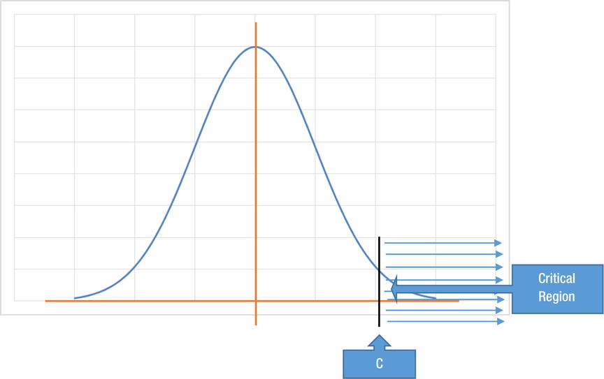
Figure 8-23. Critical region for Type 1 error
The following bullets further clarify the level of significance. The level of significance is
- The probability of Type 1 error.
- Also known as the probability of rejection error.
- Also known as the size of the test.
- Predefined probability to wrongly reject the null hypothesis.
- Minimum P-value required for accepting the null hypothesis.
Every test will begin with a level of significance, generally fixed as 5 percent, 10 percent, or 1 percent.
Type 2 Error: Accepting the Null Hypothesis When It Is False
A Type 2 error is when you wrongly accept the null hypothesis. It is also known as an acceptance error. The probability of a Type 2 error is denoted by β. For example, falling for a typical sales trap is an example of a Type 2 error. Say a salesman tries to sell you a defective product. He says that the product is really good (say the null hypothesis). If you go ahead and buy that item, then you are accepting a wrong null hypothesis. This is a Type 2 error. The probability of a Type 2 error, or β, is used for calculating the power of the test.
The following bullets clarify further the power of the test:
- 1- β
- 1-P (accepting H0 wrongly)
- 1-P (accepting H0 when H0 is false)
- P (rejecting H0 when H0 is false)
Which Error Is Worse: Type 1 or Type 2?
We simply can’t state, in general, which error is worse. It depends on the null hypothesis and the problem under consideration. Consider the two scenarios demonstrated in Table 8-11. In the first scenario, the Type 1 error is dangerous, and in the second scenario, the Type 2 error is dangerous.
Table 8-11. Which Error Is Bad? Example Scenarios
|
Scenario and Null Hypothesis |
Type 1 Error |
Type 2 Error |
|---|---|---|
|
Testing whether a drug is poison or not H0: Drug is poisonous |
The Type 1 error is rejecting the null hypothesis (saying that the drug is not poisonous) when it is really poisonous. Stating that the drug is safe might yield serious consequences. |
The Type 2 error is accepting the null hypothesis (saying that the drug is poisonous) when it is really not poisonous. Stating that the good drug is unsafe might not cause a big damage. |
|
Testing whether a customer is good or bad before giving a huge personal loan H0: Customer is good |
The Type 1 error is rejecting the null hypothesis (saying the customer is bad) when the customer is really good. You might lose one good customer and the profits associated with that customer. |
The Type 2 error is accepting the null hypothesis (saying the customer is good) when the customer is bad. If you approve one bad loan, that one bad customer could eat up 100 good customers’ profits by running away with the loan amount. |
![]() Note Though we are using the phrase “accepting the null hypothesis,” when really testing, you don’t really accept a null hypothesis. You either reject a null hypothesis or fail to reject the null hypothesis. We used “accepting the null hypothesis” to make it easier to understand.
Note Though we are using the phrase “accepting the null hypothesis,” when really testing, you don’t really accept a null hypothesis. You either reject a null hypothesis or fail to reject the null hypothesis. We used “accepting the null hypothesis” to make it easier to understand.
Conclusion
This chapter discussed one of the most applicable statistical concepts called testing a hypothesis. This concept is used even in court trials. The central limit theorem and similar theorems that explain the sampling distribution about the sampling statistic are the keys when testing a hypothesis. The P-value helps in final inference. Significance tests are used in many other statistical concepts such as regression, correlation, testing independence, testing the impact of independent variable on the dependent variable, and so on.
So far, you’ve read chapters about basic descriptive statistics, data cleaning techniques, and testing the statistical significance. In the coming chapters, you’ll learn some predictive modeling techniques such as linear regression, logistic regression, time-series forecasting, and so on.