![]()
Discovering Windowing Functions
The windowing functions, sometimes called window or windowed functions, are the most exciting features added to T-SQL over the past several versions. Starting with SQL Server 2005, the window functions, which have nothing to do with the Windows operating system, enable T-SQL developers to solve complex queries in new and innovative ways. Window functions perform calculations over a “window” or set of rows. They allow the developer to solve problems in easier and frequently better performing ways. This chapter will explain the ranking and window aggregate functions added with SQL Server 2005 and the many enhancements and new analytic functions that are part of SQL Server 2012.
What Is a Windowing Function?
Windowing functions operate on the set of the data that is returned to the client. They might perform a calculation like a SUM over all the rows without losing the details, rank the data, or pull a value from a different row without doing a self-join. For each row of the results of a query, the windowing function will perform a calculation over a window of rows. That window is defined with the OVER clause. The OVER clause is required whenever you use windowing functions.
Windowing functions are allowed only in the SELECT and ORDER BY clauses. It is important to keep this in mind as you use them in your queries. To get around this limitation, you can take advantage of CTEs to separate out the logic and filter in the outer query. The windowing functions can be divided into several types that you will learn about in the sections of this chapter:
- Ranking functions: This type of function adds a ranking for each row or divides the rows into buckets.
- Window aggregates: This function allows you to calculate summary values in a nonaggregated query.
- Accumulating aggregates: Enables the calculation of running totals.
- Analytic functions: Several new scalar functions, four of which are almost magical!
Ranking Functions
The ranking functions—ROW_NUMBER, RANK, DENSE_RANK, and NTILE—were added to SQL Server as part of SQL Server 2005. The first three assign a ranking number to each row in the result set. The NTILE function divides a set of rows into buckets.
Defining the Window
As previously mentioned, the OVER clause defines the window for the ranking function. In this case, the OVER clause must specify the order of the rows, which then determines how the function is applied to the data. The ORDER BY inside the OVER clause is not related or linked to an ORDER BY clause for the entire query.
Here is the syntax for the ROW_NUMBER, RANK, and DENSE_RANK functions, respectively:
SELECT [<col1>,][<col2>,] ROW_NUMBER() OVER(ORDER BY <col1>[,<col2>]) AS RowNum
FROM <table>;

SELECT [<col1>,][<col2>,] RANK() OVER(ORDER BY <col1>[,<col2>]) AS RankNum
FROM <table>;

SELECT [<col1>,][<col2>,] DENSE_RANK() OVER(ORDER BY <col1>[,<col2>]) AS DenseRankNum
FROM <table>;
These functions differ in how they process ties or duplicates in the ORDER BY columns. If the values of the column or combination of columns chosen are unique, then these three functions will return identical results. Type in and run the code in Listing 8-1 to learn how to use these functions.
Listing 8-1. Using the Ranking Functions
--1
SELECT CustomerID,
    ROW_NUMBER() OVER(ORDER BY CustomerID) AS RowNum,
    RANK() OVER(ORDER BY CustomerID) AS RankNum,
    DENSE_RANK() OVER(ORDER BY CustomerID) AS DenseRankNum,
    ROW_NUMBER() OVER(ORDER BY CustomerID DESC) AS ReverseRowNum
FROM Sales.Customer
WHERE CustomerID BETWEEN 11000 AND 11200
ORDER BY CustomerID;

--2
SELECT SalesOrderID, CustomerID,
    ROW_NUMBER() OVER(ORDER BY CustomerID) AS RowNum,
    RANK() OVER(ORDER BY CustomerID) AS RankNum,
    DENSE_RANK() OVER(ORDER BY CustomerID) AS DenseRankNum
FROM Sales.SalesOrderHeader
WHERE CustomerID BETWEEN 11000 AND 11200
ORDER BY CustomerID;
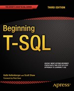
The ORDER BY option in the OVER clause of query 1 is on the CustomerID column of the Sales.Customer table. Because CustomerID is the primary key and, therefore, unique, the first three functions return the same values. The last function applies the row numbers in reverse order, which brings up an important point. The order specified in the OVER clause does not have to match the ORDER BY of the query itself.
Query 2 also has the CustomerID as the ORDER BY option, but it is not unique in the Sales.SalesOrderHeader table. Notice in Figure 8-1 that when a customer has more than one purchase, in other words the CustomerID is duplicated, the RANK and DENSE_RANK functions produce different values. After the duplicate, RANK catches up with ROW_NUMBER, while DENSE_RANK continues on with the next value.
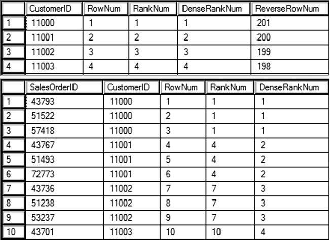
Figure 8-1. The partial results of using the ranking functions
An interesting thing to note is that ROW_NUMBER will always return a unique value within the window. RANK and DENSE_RANK will also return unique values if the ORDER BY option is unique.
Dividing the Window into Partitions
If you have a window with a view to the outside world near you, it may be divided into two or more panes. You can also divide the window used by your function into sections called partitions. This sounds a lot like the GROUP BY clause in aggregate queries, but it is very different. When you are grouping, you end up with one row in the results for each unique group. When partitioning in the OVER clause, you retain all the detail rows in the results.
For the ranking functions, partitioning means that the row or rank number will start over for each partition. When using ROW_NUMBER, the value returned will be unique within the partition. Listing 8-2 demonstrates using the PARTITION BY option of the OVER clause.
Listing 8-2. Using PARTITION BY
SELECT SalesOrderID, OrderDate, CustomerID,
    ROW_NUMBER() OVER(PARTITION BY CustomerID ORDER BY OrderDate) AS RowNum
FROM Sales.SalesOrderHeader
ORDER BY CustomerID;
Figure 8-2 shows the partial results of running this code. The row numbers start over for each customer.
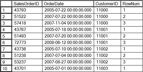
Figure 8-2. The partial results of using PARTITION BY
Using NTILE
The NTILE function works differently from other ranking functions. It assigns a number to sections of rows, evenly dividing the data into buckets. Here is the syntax for NTILE:
SELECT <col1>,NTILE(<number of buckets>) OVER([PARTITION BY <col2>] ORDER BY <col3>)
FROM <table>;
One obvious difference is that there is a required argument, the number of buckets, specified. Otherwise, the OVER clause has the same rules as the other ranking functions. The ORDER BY column is required, and the PARITION BY column is optional. Listing 8-3 shows two examples of the NTILE function.
Listing 8-3. Using the NTILE Function
SELECT SP.FirstName, SP.LastName,
    SUM(SOH.TotalDue) AS TotalSales,
    NTILE(4) OVER(ORDER BY SUM(SOH.TotalDue)) AS Bucket
FROM [Sales].[vSalesPerson] SP
JOIN Sales.SalesOrderHeader SOH ON SP.BusinessEntityID = SOH.SalesPersonID
WHERE SOH.OrderDate >= '2007-01-01' AND SOH.OrderDate < '2008-01-01'
GROUP BY FirstName, LastName
ORDER BY TotalSales;

--2
SELECT SP.FirstName, SP.LastName,
        SUM(SOH.TotalDue) AS TotalSales,
        NTILE(4) OVER(ORDER BY SUM(SOH.TotalDue)) * 1000 AS Bonus
FROM [Sales].[vSalesPerson] SP
JOIN Sales.SalesOrderHeader SOH ON SP.BusinessEntityID = SOH.SalesPersonID
WHERE SOH.OrderDate >= '2007-01-01' AND SOH.OrderDate < '2008-01-01'
GROUP BY FirstName, LastName
ORDER BY TotalSales;
Listing 8-3 is a very interesting example. It shows that you can use windowing functions in an aggregate query. In fact, an aggregate expression is used as the ORDER BY expression. Query 1 divides the salespeople into four buckets based on the 2007 sales. The salespeople with the lowest sales end up in bucket 1. The salespeople with the highest sales end up in bucket 4.
Query 2 multiplies the bucket number in each row by 1000. In this example, the manager has calculated the bonus due to each salesperson based on sales. Figure 8-3 shows the complete results of query 1 and a few of the rows from query 2. Notice that each bucket has four rows except for bucket 1, which has five rows. The NTILE function divides the data as evenly as it can. If there were 18 rows in the results, bucket 2 would also have an extra row.
Figure 8-3. The partial results of using NTILE
Complete Exercise 8-1 to practice what you have learned about the ranking functions.
Use the AdventureWorks database to complete this exercise. You can find the solutions at the end of the chapter.
- Write a query that assigns row numbers to the Production.Product table. Start the numbers over for each ProductSubCategoryID and make sure that the row numbers are in order of ProductID. Display only rows where the ProductSubCategoryID is not null.
- Write a query that divides the customers into ten buckets based on the total sales for 2005.
Summarizing Results with Window Aggregates
Also introduced with SQL Server 2005, window aggregates allow you to add aggregate expressions to nonaggregate queries. For example, you may want to see an overall total of sales along with the details of those sales.
Window aggregate functions require the OVER clause and support PARTITION BY. They do not, however, support the ORDER BY option. Listing 8-4 demonstrates how to use window aggregates.
Listing 8-4. Using Window Aggregates
--1
SELECT SalesOrderID, CustomerID,
    COUNT(*) OVER() AS CountOfSales,
    COUNT(*) OVER(PARTITION BY CustomerID) AS CountOfCustSales,
    SUM(TotalDue) OVER(PARTITION BY CustomerID) AS SumOfCustSales
FROM Sales.SalesOrderHeader
ORDER BY CustomerID;

--2
SELECT SalesOrderID, CustomerID,
    COUNT(*) OVER() AS CountOfSales,
    COUNT(*) OVER(PARTITION BY CustomerID) AS CountOfCustSales,
    SUM(TotalDue) OVER(PARTITION BY CustomerID) AS SumOfCustSales
FROM Sales.SalesOrderHeader
where SalesOrderId > 55000
ORDER BY CustomerID;
Figure 8-4 shows the partial results of running this code. Notice that the aggregate functions COUNT and SUM have been added to the query but there is no GROUP BY clause. In addition, the detail rows are returned along with the results of the aggregate functions. The empty OVER clause performs the calculation over the entire set of rows. The window defined by the empty parentheses () is the entire set of results. Notice that query 1 returns 31465 for the count of rows, while query 2 returns only 20123 rows. This is just another reminder that the aggregate functions, and all the windowing functions, operate after the WHERE clause.
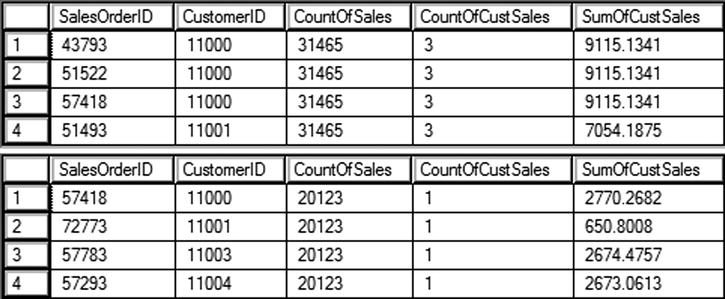
Figure 8-4. The partial results of using window aggregate expressions
When adding the PARTITION BY option to the OVER clause, the window for each calculation is now defined by the column or columns specified.
Complete Exercise 8-2 to practice what you have learned about window aggregates.
Use the AdventureWorks database to complete this exercise. You can find the solutions at the end of the chapter.
- Write a query returning the SalesOrderID, OrderDate, CustomerID, and TotalDue from the Sales.SalesOrderHeader table. Include the average order total over all the results.
- Add the average total due for each customer to the query you wrote in question 1.
Defining the Window with Framing
Starting with SQL Server 2012, you can further define the window for certain window functions with frames. You’ll see an example of how this is used in the next section. Each row in the results will have a different window for the calculation.
To understand framing, you must first learn the three key phrases UNBOUNDED PRECEDING, UNBOUNDED FOLLOWING, and CURRENT ROW. To understand what these mean and how they work, take a look at the examples in Table 8-1. Imagine that you have 100 rows in the results and you are viewing the rows from the perspective of row 10. Remember that each row in the results has its own window.
Table 8-1. Framining Examples
|
Frame Definition |
Rows in Frame for Row 10 |
|---|---|
|
ROWS BETWEEN UNBOUNDED PRECEDING AND CURRENT ROW |
Rows 1–10 |
|
ROWS BETWEEN CURRENT ROW AND UNBOUNDED FOLLOWING |
Rows 10–100 |
|
ROWS BETWEEN UNBOUNDED PRECEDING AND UNBOUNDED FOLLOWING |
Rows 1–100 |
In each of the examples in Table 8-1, the CURRENT ROW is row 10. The phrase UNBOUNDED PRECEDING means every row up to row 10. The phrase UNBOUNDED FOLLOWING means every row greater than row 10. When using framing, the ORDER BY option of the OVER clause is critical in determining which row is the first row and so on.
You can also specify an offset, or the actual number of rows removed from the current row. Table 8-2 shows how this works. Again, these examples are from the perspective of row 10 within a 100 row result set.
Table 8-2. Using Row Number Offsets
|
Frame Definition |
Rows in Frame for Row 10 |
|---|---|
|
ROWS BETWEEN 3 PRECEDING AND CURRENT ROW |
Rows 7–10 |
|
ROWS BETWEEN CURRENT ROW AND 5 FOLLOWING |
Rows 10–15 |
|
ROWS BETWEEN UNBOUNDED PRECEDING AND 5 FOLLOWING |
Rows 1–15 |
|
ROWS BETWEEN 3 PRECEDING AND 5 FOLLOWING |
Rows 7–15 |
Remember that each row in the results has its own frame. When looking at the frame from the perspective of row 9, the frame will shift to the left one row.
This section covered framing with the keyword ROWS. There is another keyword, RANGE, that can be used in place of ROWS. For the most part, they do the same thing, however, there are some differences. Window functions are part of the ANSI standards for the SQL language. Microsoft has not fully implemented everything that the ANSI standards have come up with for RANGE, so, at this time, it is much better to specify ROWS. See the section “Understanding the Difference Between ROWS and RANGE” later in the chapter to learn the differences.
Calculating Running Totals
By adding an ORDER BY clause to a window aggregate expression, you can calculate a running total. This functionality was added with SQL Server 2012. If you had tried to add the ORDER BY to a window aggregate function in an earlier version, you would have gotten an error message. The window aggregate functions require a frame, but it is RANGE BETWEEN UNBOUNDED PRECEDING AND CURRENT ROW by default if you don’t specify anything different.
Listing 8-5 shows how to calculate running totals using window functions.
Listing 8-5. Using Window Functions to Calculate Running Totals
--1
SELECT SalesOrderID, CustomerID, TotalDue,
    SUM(TotalDue) OVER(PARTITION BY CustomerID
        ORDER BY SalesOrderID)
        AS RunningTotal
FROM Sales.SalesOrderHeader
ORDER BY CustomerID, SalesOrderID;

--2
SELECT SalesOrderID, CustomerID, TotalDue,
    SUM(TotalDue) OVER(PARTITION BY CustomerID
        ORDER BY SalesOrderID
        ROWS BETWEEN CURRENT ROW AND UNBOUNDED FOLLOWING)
        AS ReverseTotal
FROM Sales.SalesOrderHeader
ORDER BY CustomerID, SalesOrderID;
Figure 8-5 shows the results for the first two customers. By adding ORDER BY to the OVER clause, the window aggregate function now accumulates the totals instead of calculating a discrete total for each row. The results are partitioned by the CustomerID column, so the running total is calculated for each customer. In query 1, the frame is not specified so the default is used. In query 2, a different frame is specified so that the reverse running total is calculated instead.
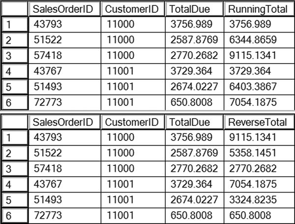
Figure 8-5. The partial results of calculating running totals
Understanding the Difference Between ROWS and RANGE
As mentioned, frames defined with ROWS and RANGE provide the same results most of the time. Besides not fully implementing RANGE, there is a difference in how these two operators work. ROWS is a physical operator, while RANGE is a logical operator. To see the difference, Listing 8-6 demonstrates how these two operators can return different results when the ORDER BY column is not unique.
Listing 8-6. Demonstrate the Difference Between ROWS and RANGE
SELECT SalesOrderID, OrderDate,CustomerID, TotalDue,
    SUM(TotalDue) OVER(PARTITION BY CustomerID
        ORDER BY OrderDate
        ROWS BETWEEN UNBOUNDED PRECEDING AND CURRENT ROW)
        AS ROWS_RT,
        SUM(TotalDue) OVER(PARTITION BY CustomerID
        ORDER BY OrderDate
        RANGE BETWEEN UNBOUNDED PRECEDING AND CURRENT ROW)
        AS RANGE_RT
FROM Sales.SalesOrderHeader
WHERE CustomerID = 29837;
Figure 8-6 shows the results of this code. Customer 29837 was chosen because it has multiple orders on the same date. By changing the ORDER BY column in the OVER clause to the nonunique OrderDate, the results of using RANGE are obvious. The ROWS operator returns a running total based on the physical position of the rows. The RANGE operator treats duplicate values the same. Because it is calculating based on the logical value, the results do not produce a true running total.
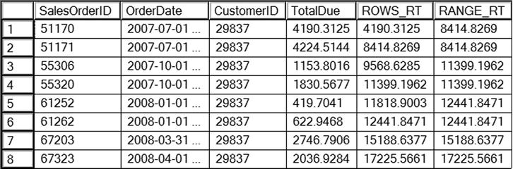
Figure 8-6. The difference between ROWS and RANGE
Notice that on 2007-07-01, two orders were placed. The ROWS_RT column adds the TotalDue as expected. The RANGE_RT treats these as logically the same, so the window for row 1 is the same as the window for row 2.
There are two things to learn from this. First, make sure that you always use a unique column or combination of columns for the ORDER BY option in the OVER clause. You should also understand that, by default, RANGE will be used if no framing option is specified. Second, make sure you always specify ROWS and don’t rely on the default value. There is also a performance difference between the two. You’ll learn more about this in the “Thinking About Performance” section later in the chapter.
Complete Exercise 8-3 to practice what you have learned about using ROWS and RANGE.
Use the AdventureWorks database to complete this exercise. You can find the solutions at the end of the chapter.
- Write a query that returns the SalesOrderID, ProductID, and LineTotal from Sales.SalesOrderDetail. Calculate a running total of the LineTotal for each ProductID. Be sure to use the correct frame.
- Explain why you should specify the frame where it is supported instead of relying on the default.
Using Window Analytic Functions
Microsoft added eight new window analytic functions with SQL Server 2012. Four of the functions deal with percentage calculations and the other four allow you to pull data from other rows.
LAG and LEAD
The two new functions LAG and LEAD are simply amazing. These functions allow you to “take a peek” at a different row. Previous to SQL Server 2012, you would have had to write poorly performing self-joins to achieve the same results. The LAG function lets you pull any column from a previous row. The LEAD function allows you to pull any column from a following row. The performance of these two functions is fantastic and framing is not supported, but partitioning is. Here is the syntax for LAG and LEAD:
SELECT <col1>[,<col2>], LAG(<column to view>) OVER(ORDER BY <col1>[,<col2>]) AS <alias>
FROM <table>;

SELECT <col1>[,<col2>], LAG(<column to view>[,<number of rows>][,<default value>]
    OVER(ORDER BY <col1>[,<col2>]) AS <alias>
FROM <table>;

SELECT <col1>[,<col2>], LEAD(<column to view>) OVER(ORDER BY <col1>[,<col2>]) AS <alias>
FROM <table>;

SELECT <col1>[,<col2>], LEAD(<column to view>[,<number of rows>][,<default value>]
    OVER(ORDER BY <col1>[,<col2>]) AS <alias>
FROM <table>;
Listing 8-7 demonstrates how to use LAG and LEAD.
Listing 8-7. Using LAG and LEAD
--1
SELECT SalesOrderID, OrderDate,CustomerID,
    LAG(OrderDate) OVER(PARTITION BY CustomerID ORDER BY SalesOrderID) AS PrevOrderDate,
    LEAD(OrderDate) OVER(PARTITION BY CustomerID ORDER BY SalesOrderID) AS FollowingOrderDate
FROM Sales.SalesOrderHeader;

--2
SELECT SalesOrderID, OrderDate,CustomerID,
    DATEDIFF(d,LAG(OrderDate,1,OrderDate)
            OVER(PARTITION BY CustomerID ORDER BY SalesOrderID), OrderDate)
            AS DaysSinceLastOrder
FROM Sales.SalesOrderHeader;
Figure 8-7 shows the partial results of running this code. Query 1 shows the default behavior of LAG and LEAD. You must specify which column you wish to see as an argument, in this case OrderDate. The ORDER BY option is required; PARTITION BY is optional. When looking at the very earliest order that was placed (Row 1 in the results), the LAG function returns NULL because there is no earlier order.
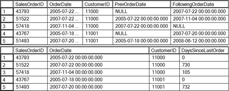
Figure 8-7. Using LAG and LEAD
Query 2 demonstrates how to use the two optional arguments. You can specify how many rows to go backward or forward, with the default of 1. The third argument is a default value to replace any NULL values. In this case, the OrderDate for the current row is specified. Query 2 also nests the LAG function within the DATEDIFF function used to calculate the number of days since the previous order.
FIRST_VALUE and LAST_VALUE
The FIRST_VALUE and LAST_VALUE functions work similarly to LAG and LEAD, but instead pull values from the very first row or very last row of the window. In this case, framing is supported. By default the frame is RANGE BETWEEN UNBOUND PRECEDING AND CURRENT ROW. Be sure to specify ROWS instead of relying on the default. When using LAST_VALUE, while you won’t get an error message with the default frame, it will not work as you expect because the default frame only goes up to the current row.
At first, this functionality seems similar to the MAX and MIN aggregate functions. They are very different, however. Instead of finding the maximum or minimum value in a set of results, they retrieve any column from the first or last row. Just like LAG and LEAD, writing a query with older techniques would have required self-joins and performed poorly. Here is the syntax:
SELECT <col1>[,<col2>], FIRST_VALUE(<column to view>)
    OVER(ORDER BY <col1>) [frame specification]
FROM <table>;

SELECT <col1>[,<col2>], LAST_VALUE(<column to view>)
    OVER(ORDER BY <col1>) frame specification
FROM <table>;
Listing 8-8 demonstrates how to use FIRST_VALUE and LAST_VALUE.
Listing 8-8. Using FIRST_VALUE and LAST_VALUE
SELECT SalesOrderID, OrderDate,CustomerID,
    FIRST_VALUE(OrderDate) OVER(PARTITION BY CustomerID ORDER BY SalesOrderID
        ROWS BETWEEN UNBOUNDED PRECEDING AND CURRENT ROW) AS FirstOrderDate,
    LAST_VALUE(OrderDate) OVER(PARTITION BY CustomerID ORDER BY SalesOrderID
        ROWS BETWEEN CURRENT ROW AND UNBOUNDED FOLLOWING) AS LastOrderDate,
        LAST_VALUE(OrderDate) OVER(PARTITION BY CustomerID ORDER BY SalesOrderID)
            AS DefaultFrame
FROM Sales.SalesOrderHeader
ORDER BY CustomerID, SalesOrderID;
Figure 8-8 shows the partial results of running this code. Notice that to get the LAST_VALUE function to work as expected, the frame must be specified. If the frame is not specified, as shown in the DefaultFrame column, the value returned in each row matches the OrderDate value for that row. That is because the default frame doesn’t go past the current row and the current row is the last value.
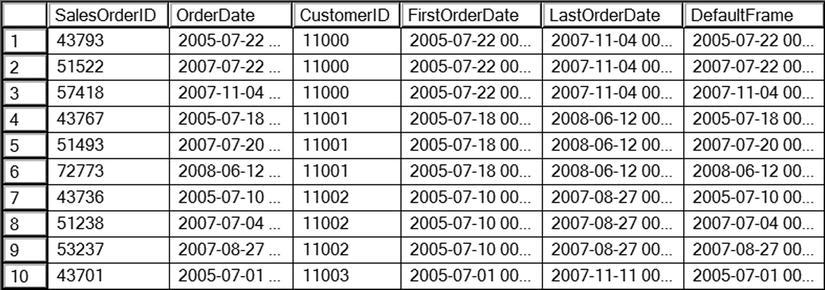
Figure 8-8. The partial results of using FIRST_VALUE and LAST_VALUE
PERCENT_RANK and CUME_DIST
The PERCENT_RANK and CUME_DIST functions are useful for statistical applications. Each of these returns a ranking over the window. For example, remember those standardized tests you took in school? The results usually gave you a ranking that showed how your score compared with the score of other students in your state or country. The ORDER BY clause is required, PARTITION BY is optional, and framing is not supported. Here is the syntax:
SELECT <col1>[,<col2>], PERCENT_RANK() OVER(ORDER BY <column or expression>)
FROM <table>;

SELECT <col1>[,<col2>], CUME_DIST() OVER(ORDER BY <column or expression>)
FROM <table>;
Type in and run Listing 8-9 to learn how to use these functions.
Listing 8-9. Using PERCENT_RANK and CUME_DIST
SELECT COUNT(*) NumberOfOrders, Month(OrderDate) AS OrderMonth,
     PERCENT_RANK() OVER(ORDER BY COUNT(*)) AS PercentRank,
     CUME_DIST() OVER(ORDER BY COUNT(*)) AS CumeDist
FROM Sales.SalesOrderHeader
GROUP BY Month(OrderDate);
Figure 8-9 shows the partial results of running this code. Notice that the two functions give slightly different results, how each month compares based on number of sales. Take a look at the sixth row in the results, January. That month had 2483 sales. The month ranked better than 45 percent of the other months. It was actually positioned at 50 percent, in other words its sales were equal to or better than 50 percent of the total sales.
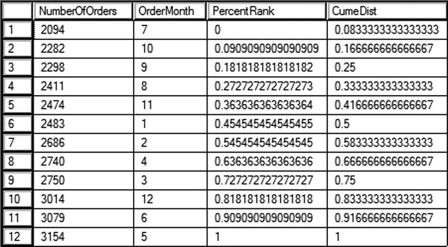
Figure 8-9. The results of using PERCENT_RANK and CUME_DIST
Another example I like to give pertains to my grandson, Thomas. He is a tall seven-year-old at the 90th percentile according to his pediatrician. That means, if I had 100 kids his age lined up by height, he would be at position 90, the cumulative distribution. He is taller than 89 kids, the percentage rank.
PERCENTILE_CONT and PERCENTILE_DISC
The PERCENTILE_CONT and PERCENTILE_DISC functions have the opposite functionality of the previously discussed two. Given a percentage rank, they figure out which value is at that position. There is also an additional clause, WITHIN GROUP, required with these functions. PERCENTILE_CONT stands for percentile continuous and PERCENTILE_DISC stands for percentile discrete. Here is the syntax:
PERCENTILE_CONT (<numeric_literal> )
    WITHIN GROUP ( ORDER BY <order_by_expression> [ ASC | DESC ] )
    OVER ( [ <partition_by_clause> ] )

PERCENTILE_DISC ( <numeric_literal> )
    WITHIN GROUP ( ORDER BY <order_by_expression> [ ASC | DESC ] )
    OVER ( [ <partition_by_clause> ] )
Another interesting thing to note is that the OVER clause does not contain the ORDER BY option. It is found in the WITHIN GROUP clause. Listing 8-10 shows how to use these functions.
Listing 8-10. Using PERCENTILE_CONT and PERCENTILE_DISC
SELECT COUNT(*) NumberOfOrders, Month(OrderDate) AS OrderMonth,
     PERCENTILE_CONT(0.5) WITHIN GROUP(ORDER BY COUNT(*)) OVER() AS PercentileCont,
     PERCENTILE_DISC(0.5) WITHIN GROUP(ORDER BY COUNT(*)) OVER() AS PercentileDisc
FROM Sales.SalesOrderHeader
GROUP BY Month(OrderDate);
Figure 8-10 shows the results of running this code. Given a set of values and a rank, these functions return the value at that rank. The difference between the two functions is that PERCENTILE_CONT will calculate the exact value if the actual value is not part of the list. In this example, if one of the months is left out so there is an odd number of rows, PERCENTILE_CONT will return the exact value in the middle of the list. The PERCENTILE_DISC function will always return an actual value from the set, the one that is closest to the rank. The results show which value is at 50 percent.
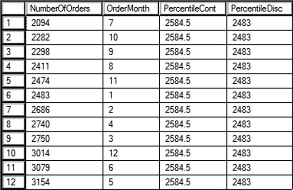
Figure 8-10. Using PERCENTILE_CONT and PERCENTILE_DISC
Complete Exercise 8-4 to learn how to use PERCENTILE_CONT and PERCENTILE_DISC.
Use the AdventureWorks database to complete this exercise. You can find the solutions at the end of the chapter. Run the following script that creates a table holding stock market data.
CREATE TABLE #Stock (Symbol VARCHAR(4), TradingDate DATE,
    OpeningPrice MONEY, ClosingPrice MONEY);
INSERT INTO #Stock(Symbol, TradingDate, OpeningPrice, ClosingPrice)
VALUES ('A','2014/01/02',5.03,4.90),
    ('B','2014/01/02',10.99,11.25),
    ('C','2014/01/02',23.42,23.44),
    ('A','2014/01/03',4.93,5.10),
    ('B','2014/01/03',11.25,11.25),
    ('C','2014/01/03',25.15,25.06),
    ('A','2014/01/06',5.15,5.20),
    ('B','2014/01/06',11.30,11.12),
    ('C','2014/01/06',25.20,26.00);
- Write a query using a window analytic function that calculates the difference in the closing price from the previous day.
- Modify the query written in question 1 so that the NULL values in the calculation are replaced with zeros. Use an option in the window analytic function.
Applying Windowing Functions
The purposes of most of the functions introduced in this chapter are obvious. When I present this topic at events like PASS Summit or SQL Saturdays, the audience is pretty excited when they see what can be done, especially with LAG, LEAD, FIRST_VALUE, and LAST_VALUE functions. I’ve heard a few say that they now have a great argument for upgrading to SQL Server 2012 or 2014 sooner rather than later. I’m not exaggerating when I talk about how powerful these functionalities are.
You may be wondering, however, about the ranking functions. Why would you ever need to use a function like ROW_NUMBER? What I have found is that I discover new reasons to use ROW_NUMBER and the other windowing functions all the time. In fact, whenever I have a difficult query to write, I often just add ROW_NUMBER and then look for patterns. Using these functions has helped me approach T-SQL from a set-based mindset instead of an iterative mindset. In this section, I’ll show you a couple of examples where these functions can help solve a tricky problem.
Removing Duplicates
One of the applications of ROW_NUMBER is to remove duplicate rows from data. The ROW_NUMBER function returns a unique number for each row in the window or set of rows returned. By adding a row number, you can turn data with duplicates into unique rows temporarily. By partitioning on all the columns, you start the numbering over for each unique combination of columns. That means that each unique row will have a row number of 1, and you can delete the rows with row numbers greater than 1. Listing 8-11 shows how to remove duplicate rows using ROW_NUMBER.
Listing 8-11. Using ROW_NUMBER() to Remove Duplicate Rows
--1
CREATE TABLE #Dupes (
    COL1 INT, Col2 INT, Col3 INT);

INSERT INTO #Dupes (Col1, Col2, Col3)
VALUES (1,1,1),(1,1,1),(1,2,3),(1,2,2),(1,2,2),
    (2,3,3),(2,3,3),(2,3,3),(2,3,3);

--2
SELECT Col1, Col2, Col3,
    ROW_NUMBER() OVER(PARTITION BY Col1, Col2, Col3 ORDER BY Col1, Col2, Col3) AS RowNum
FROM #Dupes;

--3
WITH Dupes AS (
        SELECT Col1, Col2, Col3,
          ROW_NUMBER() OVER(PARTITION BY Col1, Col2, Col3 ORDER BY Col1, Col2, Col3) AS RowNum
    FROM #Dupes)
SELECT Col1, Col2, Col3, RowNum
FROM Dupes
WHERE RowNum = 1;

--4
WITH Dupes AS (
        SELECT Col1, Col2, Col3,
          ROW_NUMBER() OVER(PARTITION BY Col1, Col2, Col3 ORDER BY Col1, Col2, Col3) AS RowNum
    FROM #Dupes)
DELETE Dupes
WHERE RowNum > 1;

--5
SELECT Col1, Col2, Col3
FROM #Dupes;
Figure 8-11 shows the results of running this code. Code section 1 creates a table and then populates it with several rows, many are duplicated. Query 2 shows the data along with a row number that is partitioned by the combination of every column. This causes the row numbers to start over for each unique row. Statement 4 removes all of the rows with row numbers over 1. Each unique set of rows has a row number 1. Because we want to keep just one row for each unique combination, deleting the rows with row numbers greater than 1 removes unneeded rows. Because it is not possible to filter on the row number directly, a CTE is used. Finally, query 5 demonstrates that the duplicates were removed.
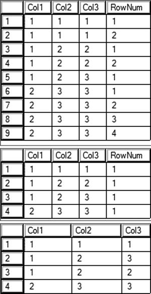
Figure 8-11. Using ROW_NUMBER() to remove duplicates
Solving an Islands Problem
The islands problem is a classic example that is difficult to solve. The purpose is to identify the boundaries of a series of data. For example, say you had the numbers 1, 2, 3, 5, 8, 9, 10, 11. The islands would be 1-3, 5, and 8-11. The gaps in the numbers are the boundaries of the islands. This technique is often used with dates, but to keep it very simple, the following example will use integers instead. Type in and run Listing 8-12 to learn this technique.
Listing 8-12. Solving an Island Problem
--1
CREATE TABLE #Island(Col1 INT);

INSERT INTO #Island (Col1)
VALUES(1),(2),(3),(5),(6),(7),(9),(9),(10);

--2
SELECT Col1, DENSE_RANK() OVER(ORDER BY COl1) AS RankNum,
       Col1 - DENSE_RANK() OVER(ORDER BY COl1) AS Diff
FROM #Island;

--3
WITH islands AS (
    SELECT Col1, Col1 - DENSE_RANK() OVER(ORDER BY COl1) AS Diff
    FROM #Island)
SELECT MIN(Col1) AS Begining, MAX(Col1) AS Ending
FROM islands
GROUP BY Diff;
Figure 8-12 shows the results of running this code. Code section 1 creates and populates a temp table. Query 2 displays the data along with the DENSE_RANK function. The DENSE_RANK function was used in this case because there are duplicates in the data. Notice that there is a pattern. Within every island, the difference between the rank and the original number is the same. For 1, 2, and 3, the first island, the difference is 0. For 5, 6, and 7, the second island, the difference is 1. Using this pattern, you can then group by the differences. The minimum and maximum values in the groups are the boundaries of the islands.
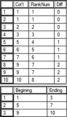
Figure 8-12. Solving an island problem
Besides making it easier for T-SQL developers to write queries, the windowing functions have been touted as having great performance over more traditional techniques. Unfortunately, you will not always see that performance boost unless you keep a few things in mind. In this section, you will learn what you need to know to get the best performance from these functions.
Indexing
Although index tuning is beyond the scope of this book, be aware that a specific type of index can help the performance of most queries that use windowing functions. This index is composed of the PARTITION BY and OVER BY columns from the OVER clause in that order. Additionally, if there are other columns listed in the SELECT list, add those as included columns to the index. Add any columns listed in the WHERE clause as index keys in front of the PARTITION BY columns.
Of course, you shouldn’t add an index to a table for every query you write, but if you do need to tune a query that contains a windowing function, this is the information you will need. The benefit of the index is to eliminate expensive sort operations.
![]() Note A debt of gratitude from the author is owed to T-SQL guru Itzik Ben-Gan for his work in educating the SQL Server community on how to get the best performance from windowing functions.
Note A debt of gratitude from the author is owed to T-SQL guru Itzik Ben-Gan for his work in educating the SQL Server community on how to get the best performance from windowing functions.
The Trouble with Window Aggregates
Window aggregate expressions are great ways to add summary calculations while retaining the details. They are very easy to write. Unfortunately, the performance is worse than when using traditional techniques. Turn on the Actual Execution Plan setting and run Listing 8-13 to see the difference.
Listing 8-13. The Difference Between Using Window Aggregates and Traditional Techniques
--1
SELECT CustomerID, SalesOrderID, TotalDue,
    SUM(TotalDue) OVER(PARTITION BY CustomerID) AS CustTotal
FROM Sales.SalesOrderHeader;

--2
;WITH Totals AS (
   SELECT CustomerID, SUM(TotalDue) AS CustTotal
   FROM Sales.SalesOrderHeader
   GROUP BY CustomerID)
SELECT Totals.CustomerID, SalesOrderID, TotalDue, CustTotal
FROM Sales.SalesOrderHeader AS SOH
INNER JOIN Totals ON SOH.CustomerID = Totals.CustomerID;
Query 1 uses the window aggregate technique to calculate a total for each customer. Query 2 uses a common table expression to first get a list of all customers and their totals. It then joins to the Sales.SalesOrderHeader table to display the same results as query 1. When you take a look at the execution you’ll see that query 1 doesn’t perform as well as query 2. While adding an index as described in the previous section can improve performance, the performance will always be worse than that for the technique used in query 2.
You can also turn on Statistics IO to see the difference. Query 1 has over 140,000 logical reads, while query 2 has about 1400 logical reads.
This doesn’t mean that you should avoid using window aggregates. It’s a fantastic technique that can make your code easy to write and maintain. It is important, however, to keep the performance penalty in mind so they can be avoided when performance is critical.
Framing
In addition to the logical differences described in the section “Understanding the Difference between ROWS and RANGE,” there is also a performance difference between ROWS and RANGE. Turn off the Actual Execution Plan, which will be identical for these queries. Run Listing 8-14 to see the differences.
Listing 8-14. Performance Differences Between ROWS and RANGE
--1
SET STATISTICS IO ON;
GO
SELECT SalesOrderID, TotalDue, CustomerID,
    SUM(TotalDue) OVER(PARTITION BY CustomerID ORDER BY OrderDate) AS RunningTotal
FROM Sales.SalesOrderHeader;

--2
SELECT SalesOrderID, TotalDue, CustomerID,
    SUM(TotalDue) OVER(PARTITION BY CustomerID ORDER BY OrderDate
            ROWS BETWEEN UNBOUNDED PRECEDING AND CURRENT ROW) AS RunningTotal
FROM Sales.SalesOrderHeader;
Query 1 calculates the running total for each customer without specifying the frame. By default, the frame will be RANGE BETWEEN UNBOUNDED PRECEDING AND CURRENT ROW. Because the ORDER BY clause is unique, there will not be any issues with the values returned. Query 2 specifies the framing clause, substituting ROWS instead of RANGE. Figure 8-13 shows the Statistics IO message, which shows that RANGE has much worse performance than ROWS. The difference has to do with how the database engine implements the worktable used to perform the calculations.
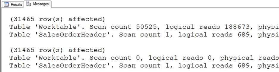
Figure 8-13. The performance difference between ROWS and RANGE
Summary
Beginning with SQL Server 2005, windowing functions have been fantastic additions to the T-SQL language. The more you work with T-SQL, the more frequently you will find reasons to use these functions.
Be sure to keep in mind the lessons found in the “Thinking About Performance” section so you can get the best performance possible from your queries.
In chapter 9 you will learn more about the WHERE clause including pattern matching and full text search.
Answers to the Exercises
This section provides answers to the exercises on writing queries using windowing functions.
Solutions to Exercise 8-1: Ranking Functions
Use the AdventureWorks database to complete this exercise.
- Write a query that assigns row numbers to the Production.Product table. Start the numbers over for each ProductSubCategoryID and make sure that the row numbers are in order of ProductID. Display only rows where the ProductSubCategoryID is not null.
SELECT ProductID, ProductSubcategoryID,
ROW_NUMBER() OVER(PARTITION BY ProductSubCategoryID
ORDER BY ProductID) AS RowNum
FROM Production.Product
WHERE ProductSubcategoryID IS NOT NULL; - Write a query that divides the customers into ten buckets based on the total sales for 2005.
SELECT CustomerID, SUM(TotalDue) AS TotalSales,
NTILE(10) OVER(ORDER BY SUM(TotalDue)) AS CustBucket
FROM Sales.SalesOrderHeader
WHERE OrderDate BETWEEN '2005/1/1' AND '2005/12/31'
GROUP BY CustomerID;
Solutions to Exercise 8-2: Summarizing Results with Window Aggregates
Use the AdventureWorks database to complete this exercise.
- Write a query returning the SalesOrderID, OrderDate, CustomerID, and TotalDue from the Sales.SalesOrderHeader table. Include the average order total over all the results.
SELECT SalesOrderID, OrderDate, TotalDue, CustomerID,
AVG(TotalDue) OVER() AS AvgTotalF
FROM Sales.SalesOrderHeader; - Add the average total due for each customer to the query you wrote in question 1.
SELECT SalesOrderID, OrderDate, TotalDue, CustomerID,
AVG(TotalDue) OVER() AS AvgTotal,
AVG(TotalDue) OVER(PARTITION BY CustomerID) AS AvgCustTotal
FROM Sales.SalesOrderHeader;
Solutions to Exercise 8-3: Understanding the Difference Between ROWS and RANGE
Use the AdventureWorks database to complete this exercise.
- Write a query that returns the SalesOrderID, ProductID, and LineTotal from Sales.SalesOrderDetail. Calculate a running total of the LineTotal for each ProductID. Be sure to use the correct frame.
SELECT SalesOrderID, ProductID, LineTotal,
SUM(LineTotal) OVER(PARTITION BY ProductID
ORDER BY SalesOrderID
ROWS BETWEEN UNBOUNDED PRECEDING AND CURRENT ROW)
AS RunningTotal
FROM Sales.SalesOrderDetail; - Explain why you should specify the frame where it is supported instead of relying on the default.
By default, the frame will be RANGE BETWEEN UNBOUNDED PRECEDING AND CURRENT ROW. This will introduce logic differences when the ORDER BY column is not unique. ROWS also performs much better than RANGE.
Solutions to Exercise 8-4: Using Window Analytic Functions
Use the AdventureWorks database to complete this exercise. Run the following script that creates a table holding stock market data.
CREATE TABLE #Stock (Symbol VARCHAR(4), TradingDate DATE,
    OpeningPrice MONEY, ClosingPrice MONEY);
INSERT INTO #Stock(Symbol, TradingDate, OpeningPrice, ClosingPrice)
VALUES ('A','2014/01/02',5.03,4.90),
    ('B','2014/01/02',10.99,11.25),
    ('C','2014/01/02',23.42,23.44),
    ('A','2014/01/03',4.93,5.10),
    ('B','2014/01/03',11.25,11.25),
    ('C','2014/01/03',25.15,25.06),
    ('A','2014/01/06',5.15,5.20),
    ('B','2014/01/06',11.30,11.12),
    ('C','2014/01/06',25.20,26.00);
- Write a query using a window analytic function that calculates the difference in the closing price from the previous day.
SELECT Symbol, TradingDate, OpeningPrice, ClosingPrice,
ClosingPrice - LAG(ClosingPrice)
OVER(PARTITION BY Symbol ORDER BY TradingDate)
AS ClosingPriceChange
FROM #Stock; - Modify the query written in question 1 so that the NULL values in the calculation are replaced with zeros. Use an option in the window analytic function.
SELECT Symbol, TradingDate, OpeningPrice, ClosingPrice,
ClosingPrice - LAG(ClosingPrice,1,ClosingPrice)
OVER(PARTITION BY Symbol ORDER BY TradingDate)
AS ClosingPriceChange
FROM #Stock;