![]()
Writing Advanced Queries
In Chapter 10 you learned how to manipulate data. In this chapter you will learn some advanced query techniques. For example, you will learn more about common table expressions (CTEs), how to write a pivot query, and more. As a beginning T-SQL developer, you may or may not need this information right away. This chapter doesn’t contain any exercises, but I encourage you to experiment and come up with your own examples for any of the features that you are interested in. Consider the information in this chapter as a head start in becoming an expert T-SQL developer.
In Chapter 6 you learned to use CTEs as one of the ways to combine the data from more than one table into one query. CTEs allow you to isolate part of the query logic or do things you could not ordinarily do, such as use an aggregate expression in an update. In these cases, you could use derived tables (see the “Using Derived Tables” section in Chapter 6), but now you will learn that CTEs are much more versatile. You can do several things with CTEs that are not possible with derived tables, such as write a recursive query. This section covers these advanced CTE features.
![]() Caution The keyword WITH appears in many other statement types. Because of this, a statement containing a CTE must be the first statement in the batch, or the previous statement must end with a semicolon. At this point, Microsoft recommends using semicolons to end T-SQL statements, but it is not required yet. Some developers start all CTE definitions with a semicolon to avoid errors. The semicolon will be required in a future version of SQL Server, so you should start using it now.
Caution The keyword WITH appears in many other statement types. Because of this, a statement containing a CTE must be the first statement in the batch, or the previous statement must end with a semicolon. At this point, Microsoft recommends using semicolons to end T-SQL statements, but it is not required yet. Some developers start all CTE definitions with a semicolon to avoid errors. The semicolon will be required in a future version of SQL Server, so you should start using it now.
Alternate CTE Syntax
Throughout the book when I have demonstrated CTEs, I have shown one particular way to name the columns, within the CTE definition. You can also specify the column names up front in a column list. When you use this method, the specified column names in the column list must be used in the outer SELECT. The list overrides the column names within the CTE definition. Here is the syntax:
;WITH <ctename> (<col1>,<col2>)
AS (SELECT <col3>,<col4) FROM <table>
SELECT <col1>,<col2>
FROM <ctename>;
Listing 11-1 demonstrates this alternate method. Type in and execute the code to learn more.
Listing 11-1. Naming Columns
;WITH myCTE ([First Name], [Last Name], [Full Name])
AS(
    SELECT FirstName, LastName, CONCAT(FirstName, ' ', LastName)
        FROM Person.Person
)
SELECT [First Name], [Last Name], [Full Name]
FROM myCTE;
In this example, the column names for the CTE are found in the column list. Notice that the third column is an expression using the CONCAT function. An alias for the expression is not required because the alias will come from the column specification. If the column list was not used, then an alias within the CTE definition would be required.
You can use CTEs to organize and isolate query logic in order to write complicated queries efficiently. You can’t nest CTEs; that is, one CTE can’t contain another CTE. You can, however, add multiple CTEs to one query. You might want to do this just to make your query more readable or possibly because writing the query this way will allow you to avoid temp tables or views. Here is the syntax:
WITH <cteName1> AS (SELECT <col1> FROM <table1>),
     <cteName2> AS (SELECT <col2> FROM <table2>),
     <cteName3> AS (SELECT <col3> FROM <table3>)
SELECT <col1>, <col2>, <col3>
FROM <cteName1> INNER JOIN <cteName2> ON <join condition1>
INNER JOIN <cteName3> ON <join condition2>
Of course, your CTE definitions can contain just about any valid SELECT statement, and your outer query can use the CTEs in any way you need to use them.
To create example data for the examples in this section, download and execute the code for Listing 11-2 as given on the book’s web site page at www.apress.com.
Listing 11-2. Create Data for This Section’s Examples
USE tempdb;
GO

IF OBJECT_ID('dbo.Employee') IS NOT NULL BEGIN
    DROP TABLE dbo.Employee;
END;
IF OBJECT_ID('dbo.Contact') IS NOT NULL BEGIN
    DROP TABLE dbo.Contact;
END;
IF OBJECT_ID('dbo.JobHistory') IS NOT NULL BEGIN
    DROP TABLE dbo.JobHistory;
END;


CREATE TABLE [Employee](
        [EmployeeID] [int] NOT NULL,
        [ContactID] [int] NOT NULL,
        [ManagerID] [int] NULL,
        [Title] [nvarchar](50) NOT NULL);

CREATE TABLE [Contact] (
        [ContactID] [int] NOT NULL,
        [FirstName] [nvarchar](50) NOT NULL,
        [MiddleName] [nvarchar](50) NULL,
        [LastName] [nvarchar](50) NOT NULL);

CREATE TABLE JobHistory(
    EmployeeID INT NOT NULL,
    EffDate DATE NOT NULL,
    EffSeq INT NOT NULL,
    EmploymentStatus CHAR(1) NOT NULL,
    JobTitle VARCHAR(50) NOT NULL,
    Salary MONEY NOT NULL,
    ActionDesc VARCHAR(20)
 CONSTRAINT PK_JobHistory PRIMARY KEY CLUSTERED
(
    EmployeeID, EffDate, EffSeq
));

GO


INSERT INTO dbo.Contact (ContactID, FirstName, MiddleName, LastName) VALUES
        (1030,'Kevin','F','Brown'),
        (1009,'Thierry','B','DHers'),
        (1028,'David','M','Bradley'),
        (1070,'JoLynn','M','Dobney'),
        (1071,'Ruth','Ann','Ellerbrock'),
        (1005,'Gail','A','Erickson'),
        (1076,'Barry','K','Johnson'),
        (1006,'Jossef','H','Goldberg'),
        (1001,'Terri','Lee','Duffy'),
        (1072,'Sidney','M','Higa'),
        (1067,'Taylor','R','Maxwell'),
        (1073,'Jeffrey','L','Ford'),
        (1068,'Jo','A','Brown'),
        (1074,'Doris','M','Hartwig'),
        (1069,'John','T','Campbell'),
        (1075,'Diane','R','Glimp'),
        (1129,'Steven','T','Selikoff'),
        (1231,'Peter','J','Krebs'),
        (1172,'Stuart','V','Munson'),
        (1173,'Greg','F','Alderson'),
        (1113,'David','N','Johnson'),
        (1054,'Zheng','W','Mu'),
        (1007, 'Ovidiu', 'V', 'Cracium'),
        (1052, 'James', 'R', 'Hamilton'),
        (1053, 'Andrew', 'R', 'Hill'),
        (1056, 'Jack', 'S', 'Richins'),
        (1058, 'Michael', 'Sean', 'Ray'),
        (1064, 'Lori', 'A', 'Kane'),
        (1287, 'Ken', 'J', 'Sanchez'),

INSERT INTO dbo.Employee (EmployeeID, ContactID, ManagerID, Title) VALUES
        (1, 1209, 16,'Production Technician - WC60'),
        (2, 1030, 6,'Marketing Assistant'),
        (3, 1002, 12,'Engineering Manager'),
        (4, 1290, 3,'Senior Tool Designer'),
        (5, 1009, 263,'Tool Designer'),
        (6, 1028, 109,'Marketing Manager'),
        (7, 1070, 21,'Production Supervisor - WC60'),
        (8, 1071, 185,'Production Technician - WC10'),
        (9, 1005, 3,'Design Engineer'),
        (10, 1076, 185,'Production Technician - WC10'),
        (11, 1006, 3,'Design Engineer'),
        (12, 1001, 109,'Vice President of Engineering'),
        (13, 1072, 185,'Production Technician - WC10'),
        (14, 1067, 21,'Production Supervisor - WC50'),
        (15, 1073, 185,'Production Technician - WC10'),
        (16, 1068, 21,'Production Supervisor - WC60'),
        (17, 1074, 185,'Production Technician - WC10'),
        (18, 1069, 21,'Production Supervisor - WC60'),
        (19, 1075, 185,'Production Technician - WC10'),
        (20, 1129, 173,'Production Technician - WC30'),
        (21, 1231, 148,'Production Control Manager'),
        (22, 1172, 197,'Production Technician - WC45'),
        (23, 1173, 197,'Production Technician - WC45'),
        (24, 1113, 184,'Production Technician - WC30'),
        (25, 1054, 21,'Production Supervisor - WC10'),
        (109, 1287, NULL, 'Chief Executive Officer'),
        (148, 1052, 109, 'Vice President of Production'),
        (173, 1058, 21, 'Production Supervisor - WC30'),
        (184, 1056, 21, 'Production Supervisor - WC30'),
        (185, 1053, 21, 'Production Supervisor - WC10'),
        (197, 1064, 21, 'Production Supervisor - WC45'),
        (263, 1007, 3, 'Senior Tool Designer'),


INSERT INTO JobHistory(EmployeeID, EffDate, EffSeq, EmploymentStatus,
    JobTitle, Salary, ActionDesc)
VALUES
    (1000,'07-31-2008',1,'A','Intern',2000,'New Hire'),
    (1000,'05-31-2009',1,'A','Production Technician',2000,'Title Change'),
    (1000,'05-31-2009',2,'A','Production Technician',2500,'Salary Change'),
    (1000,'11-01-2009',1,'A','Production Technician',3000,'Salary Change'),
    (1200,'01-10-2009',1,'A','Design Engineer',5000,'New Hire'),
    (1200,'05-01-2009',1,'T','Design Engineer',5000,'Termination'),
    (1100,'08-01-2008',1,'A','Accounts Payable Specialist I',2500,'New Hire'),
    (1100,'05-01-2009',1,'A','Accounts Payable Specialist II',2500,'Title Change'),
    (1100,'05-01-2009',2,'A','Accounts Payable Specialist II',3000,'Salary Change'),
![]() Note The CTE examples in this chapter create objects in tempdb. Keep in mind that tempdb is re-created each time the SQL service restarts, so if you restart SQL Server, you may need to re-create these objects. Alternatively, create the objects in a different database so that they will be persisted.
Note The CTE examples in this chapter create objects in tempdb. Keep in mind that tempdb is re-created each time the SQL service restarts, so if you restart SQL Server, you may need to re-create these objects. Alternatively, create the objects in a different database so that they will be persisted.
Now that you have the data for the example, type in and execute the code for Listing 11-3. This listing demonstrates how to write query with multiple CTEs.
Listing 11-3. A Query with Multiple CTEs
USE tempdb;
WITH
Emp AS(
    SELECT e.EmployeeID, e.ManagerID,e.Title AS EmpTitle,
        c.FirstName + ISNULL(' ' + c.MiddleName,'') + ' ' + c.LastName AS EmpName
    FROM dbo.Employee AS e
    INNER JOIN dbo.Contact AS c
    ON e.ContactID = c.ContactID
    ),
Mgr AS(
    SELECT e.EmployeeID AS ManagerID,e.Title AS MgrTitle,
        c.FirstName + ISNULL(' ' + c.MiddleName,'') + ' ' + c.LastName AS MgrName
    FROM dbo.Employee AS e
    INNER JOIN dbo.Contact AS c
    ON e.ContactID = c.ContactID
    )
SELECT EmployeeID, Emp.ManagerID, EmpName, EmpTitle, MgrName, MgrTitle
FROM Emp INNER JOIN Mgr ON Emp.ManagerID = Mgr.ManagerID
ORDER BY EmployeeID;
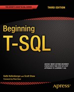
Figure 11-1 shows the partial results of running this code. Each CTE must have a name, followed by the keyword AS and the definition in parentheses. Separate the CTE definitions with a comma. This query, using tables in tempdb, contains a CTE for the employees, Emp, and a CTE for the managers, Mgr. Within each CTE, the Employee table joins the Contact table. By writing the query using CTEs, the outer query is very simple. You join the Mgr CTE to the Emp CTE just as if they were regular tables or views.
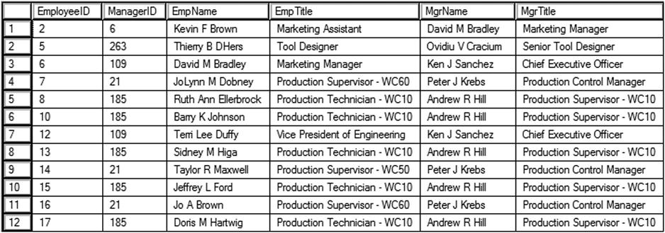
Figure 11-1. The partial results of multiple CTEs in one statement
Referencing a CTE Multiple Times
Just as you can have multiple CTE definitions within one statement, you can reference a CTE multiple times within one statement. This is not possible with a derived table, which can be used only once within a statement. (See Chapter 6 for more information about derived tables.) A CTE could be used in a self-join, in a subquery, or in any valid way of using a table within a statement. Here are two syntax examples:
--self-join
WITH <cteName> AS (SELECT <col1>, <col2> FROM <table1>)
SELECT a.<col1>, b.<col1>
FROM <cteName> AS a
INNER JOIN <cteName> AS b ON <join condition>;

--subquery
WITH <cteName> AS (SELECT <col1>, <col2> FROM <table1>)
SELECT <col1>
FROM <cteName>
WHERE <col2> IN (SELECT <col2>
    FROM <cteName> INNER JOIN <table1> ON <join condition>);
Type in and execute Listing 11-4 to see some examples. The self-join produces the same results as those in the previous section. It uses tables created in Listing 11-2.
Listing 11-4. Calling a CTE Multiple Times Within a Statement
USE tempdb;
GO
;WITH
Employees AS(
    SELECT e.EmployeeID, e.ManagerID,e.Title,
        c.FirstName + ISNULL(' ' + c.MiddleName,'') + ' ' +  c.LastName AS EmpName
    FROM dbo.Employee AS e
    INNER JOIN dbo.Contact AS c
    ON e.ContactID = c.ContactID
    )
SELECT emp.EmployeeID, emp.ManagerID, emp.EmpName, emp.Title AS EmpTitle,
   mgr.EmpName as MgrName, mgr.Title as MgrTitle
FROM Employees AS Emp INNER JOIN Employees AS Mgr
ON Emp.ManagerID = Mgr.EmployeeID;
Figure 11-2 shows the partial results of running this code. The query defines just one CTE, joining Employee to Contact. The outer query calls the CTE twice, once with the alias Emp and once with the alias Mgr.

Figure 11-2. The partial results of using a CTE twice in one statement
Joining a CTE to Another CTE
Another very interesting feature of CTEs is the ability to call one CTE from another CTE definition. This is not recursion, which you will learn about in the “Writing a Recursive Query” section. Calling one CTE from within another CTE definition allows you to base one query on a previous query. Here is a syntax example:
WITH <cteName1> AS (SELECT <col1>, <col2> FROM <table1>),
     <cteName2> AS (SELECT <col1>, <col2>, <col3>
        FROM <table3> INNER JOIN <cteName1> ON <join condition>)
SELECT <col1>, <col2>, <col3> FROM <cteName2>
The order in which the CTE definitions appear is very important. You can’t call a CTE before it is defined. Type in and execute the code in Listing 11-5 to learn more.
Listing 11-5. Joining a CTE to Another CTE
USE tempdb;
GO

--1
DECLARE @Date DATE = '05-02-2009';

--2
WITH EffectiveDate AS (
        SELECT MAX(EffDate) AS MaxDate, EmployeeID
        FROM dbo.JobHistory
        WHERE EffDate <= @Date
        GROUP BY EmployeeID
    ),
    EffectiveSeq AS (
        SELECT MAX(EffSeq) AS MaxSeq, j.EmployeeID, MaxDate
        FROM dbo.JobHistory AS j
        INNER JOIN EffectiveDate AS d
            ON j.EffDate = d.MaxDate AND j.EmployeeID = d.EmployeeID
        GROUP BY j.EmployeeID, MaxDate)
SELECT j.EmployeeID, EmploymentStatus, JobTitle, Salary
FROM dbo.JobHistory AS j
INNER JOIN EffectiveSeq AS e ON j.EmployeeID = e.EmployeeID
    AND j.EffDate = e.MaxDate AND j.EffSeq = e.MaxSeq;
Figure 11-3 shows the results of running this code. I based this example on a system I worked with for several years. Many of the tables in this system contain history information with an effective date and an effective sequence. The system adds one row to these tables for each change to the employee’s data. For a particular effective date, the system can add more than one row along with an incrementing effective sequence. To display information valid on a particular date, you first have to figure out the latest effective date before the date in mind and then figure out the effective sequence for that date. At first glance, you might think that just determining the maximum date and maximum sequence in one aggregate query should work. This doesn’t work because the maximum sequence in the table for an employee may not be valid for a particular date. For example, the employee may have four changes and, therefore, four rows for an earlier date and only one row for the latest date.

Figure 11-3. The results of calling one CTE from another CTE definition
The JobHistory table was created in tempdb including a primary key composed of EmployeeID, EffDate, and EffSeq in Listing 11-2. Notice that the insert statement inserts one row for each change even if the changes happen on the same date. Statement 1 of Listing 11-5 declares and initializes a variable, @Date, which will be used in the WHERE clause in statement 2. You can change the value of this variable to validate the results for different dates.
Statement 2 contains the SELECT statement. The first CTE, EffectiveDate, just determines the maximum EffDate from the JobHistory table for each employee that is valid for the @Date value. The second CTE, EffectiveSeq, joins the JobHistory table to the EffectiveDate CTE to find the maximum EffSeq for each employee for the date determined in the previous CTE, EffectiveDate. Finally, the outer query joins the JobHistory table on the EffectiveSeq CTE to display the valid data for each employee on the date stored in @Date.
Writing a Recursive Query
Recursive code, in any programming language, is code that calls itself. Programmers use this technique to follow paths in tree or directory structures, for example, an organization chart or family tree. When following the paths in these structures, the code must start at the root, follow each path to the end, and back up again to the next path repeatedly. In T-SQL, you can use the same technique in a CTE. Recursion, while somewhat fun to write for developers, is rarely needed. Before you decide to try recursion, make sure the problem you are trying to solve is actually a good fit. Let’s use the same Employee table created in tempdb at the beginning of the chapter to demonstrate how to use a recursive CTE. The self-join found in that table represents a hierarchical structure, the organizational chart. To view the entire hierarchy, you must start at the root, the CEO of the company, and follow every possible manager-employee path down to the lowest person. Here is the syntax for writing a recursive CTE:
WITH <cteName> (<col1>, <col2>, <col3>, level)
AS
(
    --Anchor member
    SELECT <primaryKey>,<foreignKey>,<col3>, 0 AS level
    FROM <table1>
    WHERE <foreignKey> = <startingValue>
    UNION ALL
    --Recursive member
    SELECT a.<primaryKey>,a.<foreignKey>,a.<col3>, b.level + 1
    FROM <table1> AS a
    INNER JOIN <cteName> AS b
        ON a.<foreignKey>  = b.<primaryKey>
)
SELECT <col1>,<col2>,<col3>,level
FROM <cteName> [OPTION (MAXRECURSION <number>)]
To write the recursive CTE, you must have an anchor member, which is a statement that returns the top of your intended results. This is like the root of the directory. Following the anchor member, you will write the recursive member. The recursive member actually joins the CTE that contains it to the same table used in the anchor member. The results of the anchor member and the recursive member join in a UNION ALL query. Type in and execute the code in Listing 11-6 to see how this works.
Listing 11-6. A Recursive CTE
;WITH OrgChart (EmployeeID, ManagerID, Title, Level,Node)
    AS (SELECT EmployeeID, ManagerID, Title, 0,
            CONVERT(VARCHAR(30),'/') AS Node
        FROM dbo.Employee
        WHERE ManagerID IS NULL
        UNION ALL
        SELECT Emp.EmployeeID, Emp.ManagerID, Emp.Title, OrgChart.Level + 1,
           CONVERT(VARCHAR(30), OrgChart.Node +
           CONVERT(VARCHAR(30), Emp.ManagerID) + '/')
        FROM dbo.Employee AS Emp
        INNER JOIN OrgChart  ON Emp.ManagerID = OrgChart.EmployeeID
    )
SELECT EmployeeID, ManagerID, SPACE(Level * 3) + Title AS Title, Level, Node
FROM OrgChart
ORDER BY Node;

--2 Incorrectly written Recursive CTE
;WITH OrgChart (EmployeeID, ManagerID, Title, Level,Node)
    AS (SELECT EmployeeID, ManagerID, Title, 0,
            CONVERT(VARCHAR(30),'/') AS Node
        FROM dbo.Employee
        WHERE ManagerID IS NOT NULL
        UNION ALL
        SELECT Emp.EmployeeID, Emp.ManagerID,Emp.Title, OrgChart.Level + 1,
           CONVERT(VARCHAR(30),OrgChart.Node +
              CONVERT(VARCHAR,Emp.ManagerID) + '/')
        FROM dbo.Employee AS Emp
        INNER JOIN OrgChart  ON Emp.EmployeeID = OrgChart.EmployeeID
    )
SELECT EmployeeID, ManagerID, SPACE(Level * 3) + Title AS Title, Level, Node
FROM OrgChart
ORDER BY Node OPTION (MAXRECURSION 10);
Figure 11-4 shows the partial results of query 1. Query 2 will generate an error message. Query 1 is a correctly written recursive query. The anchor member selects the EmployeeID, ManagerID, and Title from the Employee table for the CEO. The CEO is the only employee with a NULL ManagerID. The level is zero. The node column, added to help sorting, is just a slash. To get this to work, the query uses the CONVERT function to change the data type of the slash to a VARCHAR(30) because the data types in the columns of the anchor member and recursive member must match exactly. The recursive member joins Employee to the CTE, OrgChart. The query is recursive because the CTE is used inside its own definition. The regular columns in the recursive member come from the table, and the level is one plus the value of the level returned from the CTE. To sort in a meaningful way, the Node shows the ManagerID values used to get to the current employee surrounded with slashes.
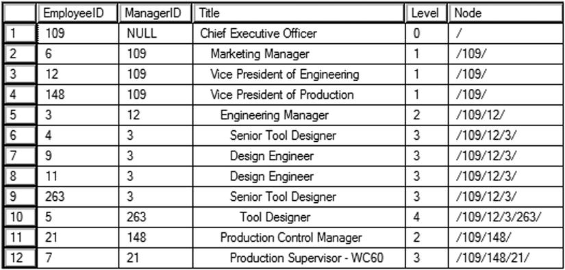
Figure 11-4. The partial results of a recursive query
The query runs the recursive member repeatedly until all possible paths are selected; that is, until the recursive member no longer returns results.
Query 2 is written incorrectly. The JOIN condition joining the anchor to the recursive member is incorrect. An incorrectly written recursive query could run in an endless loop. The recursive member will run only 100 times by default unless you specify the MAXRECURSION option to limit how many times the query will run. If the MAXRECURSION option is set to 0, it is possible to create a query that will run until you stop it. If the query will run more times than the MAXRECURSION option, an error message condition will result.
Data Manipulation with CTEs
You learned how to insert, update, and delete data in Chapter 10. You can use CTEs when modifying data, but the syntax may not be obvious at first. You perform the data modifications in the outer query whenever a CTE is used. It may be surprising, but you can also update the CTE itself. Listing 11-7 demonstrates how to use CTEs to perform inserts, updates, and deletes.
Listing 11-7. Using CTEs to Manipulate Data
--1
USE tempdb;
GO
CREATE TABLE dbo.CTEExample(CustomerID INT, FirstName NVARCHAR(50),
    LastName NVARCHAR(50), Sales Money);

--2
;WITH Cust AS(
        SELECT CustomerID, FirstName, LastName
        FROM AdventureWorks.Sales.Customer AS C
        JOIN AdventureWorks.Person.Person AS P ON C.CustomerID = P.BusinessEntityID
)
INSERT INTO dbo.CTEExample(CustomerID, FirstName, LastName)
SELECT CustomerID, FirstName, LastName
FROM Cust;

--3
;WITH Totals AS (
        SELECT CustomerID, SUM(TotalDue) AS CustTotal
        FROM AdventureWorks.Sales.SalesOrderHeader
        GROUP BY CustomerID)
UPDATE C SET Sales = CustTotal
FROM CTEExample AS C
INNER JOIN Totals ON C.CustomerID = Totals.CustomerID;

--4
;WITH Cust AS(
        SELECT CustomerID, Sales
        FROM CTEExample)
DELETE Cust
WHERE Sales < 10000;
Statement 1 creates a table for the example. The table contains the CustomerID, FirstName, LastName, and a Sales column. Statement 2 inserts rows from an AdventureWorks query within the CTE supplying the CustomerID and names. Usually when inserting data from a query, the word INSERT is first. When using a CTE, the statement begins with the CTE and then it is used in the outer query as any other table.
Statement 3 updates the table with an aggregate expression, SUM(TotalDue). It is important to note that it is not possible to update directly with an aggregate, so you must come up with some way to isolate the aggregate query. This is just one way to do it. You could create a temporary work table or use a derived table instead.
Statement 4 is very interesting. Not only is it using a CTE to delete some rows, it is actually deleting rows from the CTE itself.
Isolating Aggregate Query Logic
Several techniques exist that allow you to separate an aggregate query from the rest of the statement. Sometimes this is necessary because the grouping levels and the columns that must be displayed are not compatible. For example, you may need to show details along with summary expressions. This section will demonstrate these techniques.
Correlated Subqueries in the SELECT list
You may see correlated subqueries used within the SELECT list. I really don’t recommend this technique because if the query contains more than one correlated subquery, performance deteriorates quickly. You will learn about better options to use later in this section. Here is the syntax for the SELECT list correlated subquery:
SELECT <select list>,
    (SELECT <aggregate function>(<col1>)
     FROM <table2> WHERE <col2> = <table1>.<col3>) AS <alias name>
FROM <table1>
The subquery must produce only one row for each row of the outer query, and only one expression may be returned from the subquery. The subquery executes once for each row of the outer query. Listing 11-8 shows two examples of this query type.
Listing 11-8. Using a Correlated Subquery in the SELECT List
USE AdventureWorks;
GO
SELECT CustomerID, C.StoreID, C.AccountNumber,
    (SELECT COUNT(*)
     FROM Sales.SalesOrderHeader AS SOH
     WHERE SOH.CustomerID = C.CustomerID) AS CountOfSales
FROM Sales.Customer AS C
ORDER BY CountOfSales DESC;

--2
SELECT CustomerID, C.StoreID, C.AccountNumber,
    (SELECT COUNT(*) AS CountOfSales
     FROM Sales.SalesOrderHeader AS SOH
     WHERE SOH.CustomerID = C.CustomerID) AS CountOfSales,
    (SELECT SUM(TotalDue)
     FROM Sales.SalesOrderHeader AS SOH
     WHERE SOH.CustomerID = C.CustomerID) AS SumOfTotalDue,
    (SELECT AVG(TotalDue)
     FROM Sales.SalesOrderHeader AS SOH
     WHERE SOH.CustomerID = C.CustomerID) AS AvgOfTotalDue
FROM Sales.Customer AS C
ORDER BY CountOfSales DESC;
You can see the partial results of running this code in Figure 11-5. Query 1 demonstrates how the correlated subquery returns one value per row. Notice the WHERE clause in the subquery. The CustomerID column in the subquery must be equal to the CustomerID in the outer query. The alias for the column must be added right after the subquery definition, not the column definition.

Figure 11-5. Using a correlated subquery in the SELECT list
Normally, when working with the same column name from two tables, both must be qualified. Within the subquery, if the column is not qualified, the column is assumed to be from the table within the subquery. As a best practice, always qualify both tables in a correlated subquery.
Notice that query 2 contains three correlated subqueries because three values are required. Although one correlated subquery doesn’t usually cause a problem, performance quickly deteriorates as additional correlated subqueries are added to the query. Luckily, other techniques exist to get the same results with better performance.
Using Derived Tables
In Chapter 6 you learned about derived tables. You can use derived tables to isolate the aggregate query from the rest of the query. Here is the syntax:
SELECT <col1>,<col4>,<col3> FROM <table1> AS a
INNER JOIN
    (SELECT <aggregate function>(<col2>) AS <col4>,<col3>
     FROM <table2> GROUP BY <col3>) AS <ALIAS> ON a.<col1> = b.<col3>
Listing 11-9 shows how to use this technique. Type in and execute the code.
Listing 11-9. Using a Derived Table
SELECT c.CustomerID, c.StoreID, c.AccountNumber, s.CountOfSales,
    s.SumOfTotalDue, s.AvgOfTotalDue
FROM Sales.Customer AS c INNER JOIN
    (SELECT CustomerID, COUNT(*) AS CountOfSales,
         SUM(TotalDue) AS SumOfTotalDue,
         AVG(TotalDue) AS AvgOfTotalDue
     FROM Sales.SalesOrderHeader
     GROUP BY CustomerID) AS s
ON c.CustomerID = s.CustomerID;
You can see the partial results of running this code in Figure 11-6. This query has much better performance than the second query in Listing 11-8, but it produces the same results. Remember that any column required in the outer query must be listed in the derived table. You must also supply an alias for the derived table.
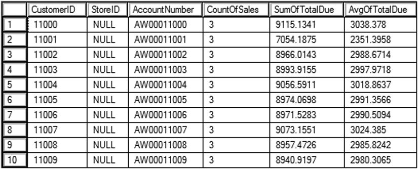
Figure 11-6. The partial results of using a derived table
Besides the increase in performance, the derived table may return more than one row for each row of the outer query in some situations, and multiple aggregates may be included.
Common Table Expressions
A CTE also allows you to isolate the aggregate query from the rest of the statement. The CTE is not stored as an object; it just makes the data available during the query. You can think of it as a temporary view. Here is the syntax:
WITH <cteName> AS (SELECT <aggregate function>(<col2>) AS <col4>, <col3>
   FROM <table2> GROUP BY <col3>)
SELECT <col1>,<col4>,<col3>
FROM <table1> INNER JOIN b ON <cteName>.<col1> = <table1>.<col3>;
Type in and execute the code in Listing 11-10 to learn how to use a CTE with an aggregate query.
Listing 11-10. Using a Common Table Expression
;WITH s AS
    (SELECT CustomerID, COUNT(*) AS CountOfSales,
        SUM(TotalDue) AS SumOfTotalDue,
        AVG(TotalDue) AS AvgOfTotalDue
     FROM Sales.SalesOrderHeader
     GROUP BY CustomerID)
SELECT c.CustomerID, c.StoreID, c.AccountNumber, s.CountOfSales,
    s.SumOfTotalDue, s.AvgOfTotalDue
FROM Sales.Customer AS c INNER JOIN s
ON c.CustomerID = s.CustomerID;
Figure 11-7 displays the results of running this code. This query looks a lot like the one in Listing 11-9. The only difference is that this query uses a CTE instead of a derived table. At this point, there is no real advantage to the CTE over the derived table, but it is easier to read, in my opinion.
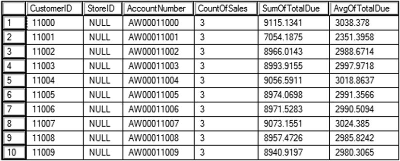
Figure 11-7. Using a common table expression
Using CROSS APPLY and OUTER APPLY
The CROSS APPLY and OUTER APPLY techniques were originally intended to enable joining to table-valued functions (see Chapter 14). They can, however, be used similarly to join to a derived table. The function or subquery on the right will be called once for every row from the table on the left. Use OUTER APPLY like a LEFT OUTER JOIN to return a row from the left even if there is nothing returned from the right. Listing 11-11 shows an example.
Listing 11-11. Using CROSS APPLY
--1
SELECT SOH.CustomerID, SOH.OrderDate, SOH.TotalDue, CRT.RunningTotal
FROM Sales.SalesOrderHeader AS SOH
CROSS APPLY(
    SELECT SUM(TotalDue) AS RunningTotal
        FROM Sales.SalesOrderHeader RT
        WHERE RT.CustomerID = SOH.CustomerID
           AND RT.SalesOrderID <= SOH.SalesOrderID) AS CRT
ORDER BY SOH.CustomerID, SOH.SalesOrderID;

--2
SELECT Prd.ProductID, S.SalesOrderID
FROM Production.Product AS Prd
OUTER APPLY (
  SELECT TOP(2) SalesOrderID
  FROM Sales.SalesOrderDetail AS SOD
  WHERE SOD.ProductID = Prd.ProductID
  ORDER BY SalesOrderID) AS S
 ORDER BY Prd.ProductID;
Query 1 returns a list of customers and their orders along with a running total (see Figure 11-8). The inner query joins to the outer query on the CustomerID and the OrderID where the OrderID is less than or equal to the OrderID from the outer query. The inner query will run once for each row of the outer query. As you may guess, this technique generally does not perform well for large tables. See Chapter 8 to see a much better way to get the same results if you are using SQL Server 2012 or later.
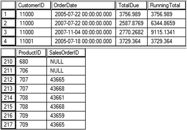
Figure 11-8. The partial results of CROSS APPLY and OUTER APPLY
Query 2 returns a list of the products along with the OrderID of the first two orders placed, if any, for that product. Because it uses OUTER APPLY, all products are returned even if no order has been placed. Figure 11-8 shows the partial results of running this code.
The OUTPUT Clause
You learned how to manipulate data in Chapter 10. The OUTPUT clause allows you to see or even save the modified values when you perform a data manipulation statement. The interesting thing about OUTPUT is that data manipulation statements don’t normally return data except for a message stating the number of rows affected. By using OUTPUT, you can retrieve a result set of the data in the same statement that updates the data. You can see the result set in the query window results or return the result set to a client application.
Using OUTPUT to View Data
When using OUTPUT, you can view the data using the special tables DELETED and INSERTED. Triggers also use DELETED and INSERTED tables. You may wonder why there is not an UPDATED table. Instead of an UPDATED table, you will find the old values in the DELETED table and the new values in the INSERTED table. Here are the syntax examples for using the OUTPUT clause for viewing changes when running data manipulation statements:
--Update style 1
UPDATE a SET <col1> = <value>
OUTPUT deleted.<col1>,inserted.<col1>
FROM <table1> AS a

--Update style 2
UPDATE <table1> SET <col1> = <value>
OUTPUT deleted.<col1>, inserted.<col1>
WHERE <criteria>

--Insert style 1
INSERT [INTO] <table1> (<col1>,<col2>)
OUTPUT inserted.<col1>, inserted.<col2>
SELECT <col1>, <col2>
FROM <table2>

--Insert style 2
INSERT [INTO] <table1> (<col1>,<col2>)
OUTPUT inserted.<col1>, inserted.<col2>
VALUES (<value1>,<value2>)

--Delete style 1
DELETE [FROM] <table1>
OUTPUT deleted.<col1>, deleted.<col2>
WHERE <criteria>

--DELETE style 2
DELETE [FROM] a
OUTPUT deleted.<col1>, deleted.<col2>
FROM <table1> AS a
Probably the trickiest thing about using OUTPUT is figuring out where in the statement to include it. Type in and execute the code in Listing 11-12 to learn more about OUTPUT.
Listing 11-12. Viewing the Manipulated Data with OUTPUT
--1
USE tempdb;
GO
IF OBJECT_ID('dbo.Customers') IS NOT NULL BEGIN
    DROP TABLE dbo.Customers;
END;

CREATE TABLE dbo.Customers (CustomerID INT NOT NULL PRIMARY KEY,
    Name VARCHAR(150),PersonID INT NOT NULL);
GO

--2
INSERT INTO dbo.Customers(CustomerID,Name,PersonID)
OUTPUT inserted.CustomerID,inserted.Name
SELECT c.CustomerID, p.FirstName + ' ' + p.LastName, c.PersonID
FROM AdventureWorks.Sales.Customer AS c
INNER JOIN AdventureWorks.Person.Person AS p
ON c.PersonID = p.BusinessEntityID;

--3
UPDATE c SET Name = p.FirstName +
    ISNULL(' ' + p.MiddleName,'') + ' ' + p.LastName
OUTPUT deleted.CustomerID,deleted.Name AS OldName, inserted.Name AS NewName
FROM dbo.Customers AS c
INNER JOIN AdventureWorks.Person.Person AS p on c.PersonID = p.BusinessEntityID;

--4
DELETE FROM dbo.Customers
OUTPUT deleted.CustomerID, deleted.Name, deleted.PersonID
WHERE CustomerID = 11000;
Figure 11-9 shows the partial results of running this code. Unfortunately, for the demo, you can’t add an ORDER BY clause to OUTPUT, and the INSERT statement, on my machine, returns the rows in a different order than the UPDATE statement. Code section 1 creates the dbo.Customers table in tempdb. Statement 2 inserts all the rows when joining the Sales.Customer table to the Person.Person table in the AdventureWorks database. You may have to adjust the name of the database if yours has the version number appended. The OUTPUT clause, located right after the INSERT clause, returns the CustomerID and Name. Statement 3 modifies the value in the Name column by including the MiddleName in the expression. The DELETED table displays the Name column data before the update. The INSERTED table displays the Name column after the update. The UPDATE clause includes aliases to differentiate the values. Statement 4 deletes one row from the table. The OUTPUT clause displays the deleted data.
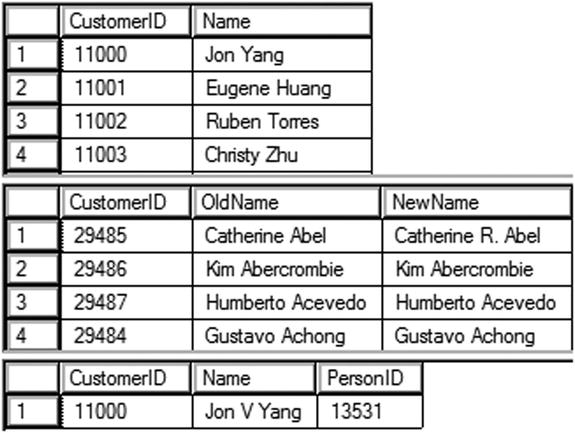
Figure 11-9. The partial results of viewing the manipulated data with OUTPUT
Saving OUTPUT Data to a Table
Instead of displaying or returning the rows from the OUTPUT clause, you might need to save the information in another table. For example, you may need to populate a history table or save the changes for further processing. Here is a syntax example showing how to use INTO along with OUTPUT:
INSERT [INTO] <table1> (<col1>, <col2>)
OUTPUT inserted.<col1>, inserted.<col2>
    INTO <table2>
SELECT <col3>,<col4>
FROM <table3>
Type in and execute the code in Listing 11-13 to learn more.
Listing 11-13. Saving the Results of OUTPUT
Use tempdb;
GO
--1
IF OBJECT_ID('dbo.Customers') IS NOT NULL BEGIN
    DROP TABLE dbo.Customers;
END;

IF OBJECT_ID('dbo.CustomerHistory') IS NOT NULL BEGIN
    DROP TABLE dbo.CustomerHistory;
END;

CREATE TABLE dbo.Customers (CustomerID INT NOT NULL PRIMARY KEY,
    Name VARCHAR(150),PersonID INT NOT NULL);

CREATE TABLE dbo.CustomerHistory(CustomerID INT NOT NULL PRIMARY KEY,
    OldName VARCHAR(150), NewName VARCHAR(150),
    ChangeDate DATETIME);
GO

--2
INSERT INTO dbo.Customers(CustomerID, Name, PersonID)
SELECT c.CustomerID, p.FirstName + ' ' + p.LastName,PersonID
FROM AdventureWorks.Sales.Customer AS c
INNER JOIN AdventureWorks.Person.Person AS p
ON c.PersonID = p.BusinessEntityID;

--3
UPDATE c SET Name = p.FirstName +
    ISNULL(' ' + p.MiddleName,'') + ' ' + p.LastName
OUTPUT deleted.CustomerID,deleted.Name, inserted.Name, GETDATE()
INTO dbo.CustomerHistory
FROM dbo.Customers AS c
INNER JOIN AdventureWorks.Person.Person AS p on c.PersonID = p.BusinessEntityID;

--4
SELECT CustomerID, OldName, NewName,ChangeDate
FROM dbo.CustomerHistory
ORDER BY CustomerID;
Figure 11-10 shows the partial results of running this code. Code section 1 creates the two tables used in this example in tempdb. Statement 2 inserts data from AdventureWorks into the new Customer table. Statement 3 updates the Name column for all of the rows. By including OUTPUT INTO, the CustomerID along with the previous and current Name values are saved into the CustomerHistory table. The statement also populates the ChangeDate column by using the GETDATE function. Statement 4 returns the rows that have been saved.
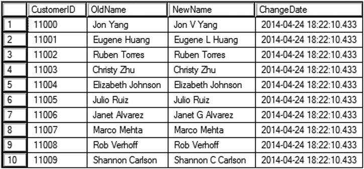
Figure 11-10. The partial results of saving the OUTPUT data into a table
The MERGE Statement
The MERGE statement, also known as upsert, allows you to bundle INSERT, UPDATE, and DELETE operations into a single statement to perform complex operations such as synchronizing the contents of one table with another. For example, you would normally need to perform at least one UPDATE, one INSERT, and one DELETE statement to keep the data in one table up to date with the data from another table. By using MERGE, you can perform the same work more efficiently (assuming that the tables have the proper indexes in place) with just one statement. The drawback is that MERGE is more difficult to understand and write than the three individual statements. One potential use for MERGE—where taking the time to write the MERGE statements really pays off—is loading data warehouses and data marts. Here is the syntax for a simple MERGE statement:
MERGE <target table>
USING <source table name>|<query> AS alias [(column names)]
ON (<join criteria>)
WHEN MATCHED [AND <other criteria>]
THEN UPDATE SET <col> = alias.<value>
WHEN NOT MATCHED BY TARGET [AND <other criteria>]
THEN INSERT (<column list>) VALUES (<values>) –- row is inserted into target
WHEN NOT MATCHED BY SOURCE [AND <other criteria>]
THEN DELETE –- row is deleted from target
[OUTPUT $action, DELETED.*, INSERTED.*];
At first glance, the syntax may seem overwhelming. Basically, it defines an action to perform if a row from the source table matches the target table (WHEN MATCHED), an action to perform if a row is missing in the target table (WHEN NOT MATCHED BY TARGET), and an action to perform if an extra row is in the target table (WHEN NOT MATCHED BY SOURCE). The actions to perform on the target table can be anything you need to do. For example, if the source table is missing a row that appears in the target table (WHEN NOT MATCHED BY SOURCE), you don’t have to delete the target row. You could, in fact, leave out that part of the statement or perform another action. In addition to the join criteria, you can also specify any other criteria in each match specification. You can include an optional OUTPUT clause along with the $action option. The $action option shows you which action is performed on each row. Include the DELETED and INSERTED tables in the OUTPUT clause to see the before and after values. The MERGE statement must end with a semicolon. Type in and execute the code in Listing 11-14 to learn how to use MERGE.
Listing 11-14. Using the MERGE Statement
USE tempdb;
GO
--1
IF OBJECT_ID('dbo.CustomerSource') IS NOT NULL BEGIN
    DROP TABLE dbo.CustomerSource;
END;
IF OBJECT_ID('dbo.CustomerTarget') IS NOT NULL BEGIN
    DROP TABLE dbo.CustomerTarget;
END;

CREATE TABLE dbo.CustomerSource (CustomerID INT NOT NULL PRIMARY KEY,
    Name VARCHAR(150) NOT NULL, PersonID INT NOT NULL);
CREATE TABLE dbo.CustomerTarget (CustomerID INT NOT NULL PRIMARY KEY,
    Name VARCHAR(150) NOT NULL, PersonID INT NOT NULL);

--2
INSERT INTO dbo.CustomerSource(CustomerID,Name,PersonID)
SELECT CustomerID,
    p.FirstName + ISNULL(' ' + p.MiddleName,'') + ' ' + p.LastName,
    c.PersonID
FROM AdventureWorks.Sales.Customer AS c
INNER JOIN AdventureWorks.Person.Person AS p ON c.PersonID = p.BusinessEntityID
WHERE c.CustomerID IN (29485,29486,29487,20075);

--3
INSERT INTO dbo.CustomerTarget(CustomerID,Name,PersonID)
SELECT c.CustomerID, p.FirstName  + ' ' + p.LastName, PersonID
FROM AdventureWorks.Sales.Customer AS c
INNER JOIN AdventureWorks.Person.Person AS p ON c.PersonID = p.BusinessEntityID
WHERE c.CustomerID IN (29485,29486,21139);

--4
SELECT CustomerID, Name, PersonID
FROM dbo.CustomerSource
ORDER BY CustomerID;


--5
SELECT CustomerID, Name, PersonID
FROM dbo.CustomerTarget
ORDER BY CustomerID;

--6
MERGE dbo.CustomerTarget AS t
USING dbo.CustomerSource AS s
ON (s.CustomerID = t.CustomerID)
WHEN MATCHED AND s.Name <> t.Name
THEN UPDATE SET Name = s.Name
WHEN NOT MATCHED BY TARGET
THEN INSERT (CustomerID, Name, PersonID) VALUES (CustomerID, Name, PersonID)
WHEN NOT MATCHED BY SOURCE
THEN DELETE
OUTPUT $action, DELETED.*, INSERTED.*;--semi-colon is required

--7
SELECT CustomerID, Name, PersonID
FROM dbo.CustomerTarget
ORDER BY CustomerID;
Figure 11-11 shows the results of running this code. Code section 1 creates the dbo.CustomerSource and dbo.CustomerTarget tables in tempdb. They have the same column names, but this is not a requirement. Statement 2 populates the dbo.CustomerSource table with four rows. It creates the Name column using the FirstName, MiddleName, and LastName columns. Statement 3 populates the dbo.CustomerTarget table with three rows. Two of the rows contain the same customers as the dbo.CustomerSource table. Query 4 displays the data from dbo.CustomerSource, and query 5 displays the data from dbo.CustomerTarget.

Figure 11-11. The results of using MERGE
Statement 6 synchronizes dbo.CustomerTarget with dbo.CustomerSource, correcting the Name column, inserting missing rows, and deleting extra rows by using the MERGE command. The statement will update dob.CustomerTarget with data from dbo.CustomerSource. The rows are matched on CustomerID. The WHEN MATCHED clause specifies what to do when there is a match between the two tables. If the Name values do not match, then change the value to the value of the Name from the source. The WHEN NOT MATCHED BY TARGET clause specifies what to do when there is a row in the source that doesn’t match the target. In this case, a row will be inserted into the target. Finally, the WHEN NOT MATCHED BY SOURCE clause specifies what to do when a row in the target doesn’t have a match in the source. In this case, the row is removed from the target table. Because the query includes the OUTPUT clause, you can see the action performed on each row. Query 7 displays the dbo.CustomerTarget with the changes. The target table now matches the source table.
GROUPING SETS
You learned all about aggregate queries in Chapter 7. Another option, GROUPING SETS, when added to an aggregate query, allows you to combine different grouping levels within one statement. This is equivalent to combining multiple aggregate queries with UNION. For example, suppose you want the data summarized by one column combined with the data summarized by a different column. Just like MERGE, this feature is very valuable for loading data warehouses and data marts. When using GROUPING SETS instead of UNION, you can see increased performance, especially when the query includes a WHERE clause and the number of columns specified in the GROUPING SETS clause increases. Here is the syntax:
SELECT <col1>,<col2>,<aggregate function>(<col3>)
FROM <table1>
WHERE <criteria>
GROUP BY GROUPING SETS (<col1>,<col2>)
Listing 11-15 compares the equivalent UNION query to a query using GROUPING SETS. Type in and execute the code to learn more.
Listing 11-15. Using GROUPING SETS
USE AdventureWorks;
GO
--1
SELECT NULL AS SalesOrderID, SUM(UnitPrice)AS SumOfPrice, ProductID
FROM Sales.SalesOrderDetail
WHERE SalesOrderID BETWEEN 44175 AND 44178
GROUP BY ProductID
UNION ALL
SELECT SalesOrderID,SUM(UnitPrice), NULL
FROM Sales.SalesOrderDetail
WHERE SalesOrderID BETWEEN 44175 AND 44178
GROUP BY SalesOrderID;

--2
SELECT SalesOrderID, SUM(UnitPrice) AS SumOfPrice,ProductID
FROM Sales.SalesOrderDetail
WHERE SalesOrderID BETWEEN 44175 AND 44178
GROUP BY GROUPING SETS(SalesOrderID, ProductID);
Figure 11-12 shows the results of running this code. Query 1 is a UNION query that calculates the sum of the UnitPrice. The first part of the query supplies a NULL value for SalesOrderID. That is because SalesOrderID is just a placeholder. The query groups by ProductID, and SalesOrderID is not needed. The second part of the query supplies a NULL value for ProductID. In this case, the query groups by SalesOrderID, and ProductID is not needed. The UNION query combines the results. Query 2 demonstrates how to write the equivalent query using GROUPING SETS.
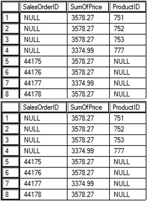
Figure 11-12. The results of comparing UNION to GROUPING SETS
CUBE and ROLLUP
You can add subtotals to your aggregate queries by using CUBE or ROLLUP in the GROUP BY clause. CUBE and ROLLUP are very similar, but there is a subtle difference. CUBE will give subtotals for every possible combination of the grouping levels. ROLLUP will give subtotals for the hierarchy. For example, if you are grouping by three columns, CUBE will provide subtotals for every grouping column. ROLLUP will provide subtotals for the first two columns but not the last column in the GROUP BY list. Here is the syntax:
SELECT <col1>, <col2>, <aggregate expression>
     FROM <table>
GROUP BY <CUBE or ROLLUP>(<col1>,<col2>)
The following example demonstrates how to use CUBE and ROLLUP. Run the code in Listing 11-16 to see how this works.
Listing 11-16. Using CUBE and ROLLUP
--1
SELECT COUNT(*) AS CountOfRows,
    ISNULL(Color, CASE WHEN GROUPING(Color)=0 THEN 'UNK' ELSE 'ALL' END) AS Color,
        ISNULL(Size,CASE WHEN GROUPING(Size) = 0 THEN 'UNK' ELSE 'ALL' END) AS Size
FROM Production.Product
GROUP BY CUBE(Color,Size)
ORDER BY Size, Color;

--2
SELECT COUNT(*) AS CountOfRows,
    ISNULL(Color, CASE WHEN GROUPING(Color)=0 THEN 'UNK' ELSE 'ALL' END) AS Color,
        ISNULL(Size,CASE WHEN GROUPING(Size) = 0 THEN 'UNK' ELSE 'ALL' END) AS Size
FROM Production.Product
GROUP BY ROLLUP(Color,Size)
ORDER BY Size, Color;
Figure 11-13 shows the partial results of running this code. Query 1 returns 98 rows while query 2 returns only 79 rows. Notice that query 1 has subtotal rows for size 38 and 40 while query 2 does not, denoted by the word ALL in the Color column. These queries use the GROUPING function, which returns a 1 if it is a summary row or 0 if it is not. This is combined with the ISNULL function so that it is only applied on the rows with actual null values or the summary rows. Scroll down in the data to find the rows where the color column is summarized.
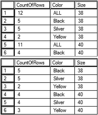
Figure 11-13. The partial results of CUBE and ROLLUP
Normally a query displays the data in a way that is similar to how it looks in a table, often with the column headers being the actual names of the columns within the table. A pivoted query displays the values of one column as column headers instead. For example, you could display the sum of the sales by month so that the month names are column headers. Each row would then contain the data by year with the sum for each month displayed from left to right. This section shows how to write pivoted queries with two techniques: CASE and PIVOT.
Pivoting Data with CASE
Many developers still use the CASE function to create pivoted results. (See “The Case Expression” section in Chapter 4 to learn more about CASE.) Essentially, you use several CASE expressions in the query, one for each pivoted column header. For example, the query could have a CASE expression checking to see whether the month of the order date is January. If the order does occur in January, it returns the total sales value. If not, it supplies a zero. For each row, the data ends up in the correct column where it can be aggregated. Here is the syntax for using CASE to pivot data:
CASE <col1>,SUM(CASE <col3> WHEN <value1> THEN <col2> ELSE 0 END) AS <alias1>,
    SUM(CASE <col3> WHEN <value2> THEN <col2> ELSE 0 END) AS <alias2>,
    SUM(CASE <col3> WHEN <value3> THEN <col2> ELSE 0 END) AS <alias3>
FROM <table1>
GROUP BY <col1>
Type in and execute Listing 11-17 to learn how to pivot data using CASE.
Listing 11-17. Using CASE to Pivot Data
SELECT YEAR(OrderDate) AS OrderYear,
ROUND(SUM(CASE MONTH(OrderDate) WHEN 1 THEN TotalDue ELSE 0 END),0)
    AS Jan,
ROUND(SUM(CASE MONTH(OrderDate) WHEN 2 THEN TotalDue ELSE 0 END),0)
    AS Feb,
ROUND(SUM(CASE MONTH(OrderDate) WHEN 3 THEN TotalDue ELSE 0 END),0)
    AS Mar,
ROUND(SUM(CASE MONTH(OrderDate) WHEN 4 THEN TotalDue ELSE 0 END),0)
    AS Apr,
ROUND(SUM(CASE MONTH(OrderDate) WHEN 5 THEN TotalDue ELSE 0 END),0)
    AS May,
ROUND(SUM(CASE MONTH(OrderDate) WHEN 6 THEN TotalDue ELSE 0 END),0)
    AS Jun
FROM Sales.SalesOrderHeader
GROUP BY YEAR(OrderDate)
ORDER BY OrderYear;
Figure 11-14 shows the results of running this code. To save space in the results, the statement calculates the totals only for the months January through June and uses the ROUND function. The GROUP BY clause contains just the YEAR(OrderDate) expression. You might think that you need to group by month as well, but this query doesn’t group by month. It just includes each TotalDue value in a different column depending on the month.
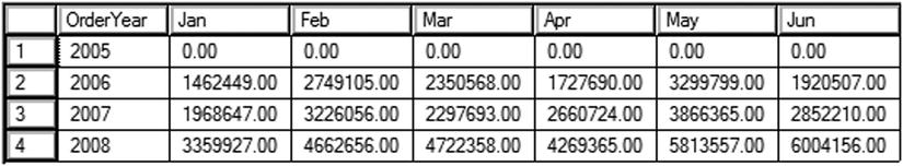
Figure 11-14. The results of using CASE to create a pivot query
Microsoft introduced the PIVOT function with SQL Server 2005. In my opinion, the PIVOT function is more difficult to understand than using CASE to produce the same results. Just like CASE, you have to hard-code the column names. This works fine when the pivoted column names will never change, such as the months of the year. When the query bases the pivoted column on data that changes over time, such as employee or department names, the query must be modified each time that data changes. Here is the syntax for PIVOT:
SELECT <groupingCol>, <pivotedValue1> [AS <alias1>], <pivotedValue2> [AS <alias2>]
FROM (SELECT <groupingCol>, <value column>, <pivoted column>) AS <queryAlias>
PIVOT
( <aggregate function>(<value column>)
FOR <pivoted column> IN (<pivotedValue1>,<pivotedValue2>)
) AS <pivotAlias>
[ORDER BY <groupingCol>]
The SELECT part of the query lists any non-pivoted columns along with the values from the pivoted column. These values from the pivoted column will become the column names in your query. You can use aliases if you want to use a different column name than the actual value. For example, if the column names will be the month numbers, you can alias with the month names.
This syntax uses a derived table, listed after the word FROM, as the basis of the query. See the “Using Derived Tables” section in Chapter 6 to review derived tables. Make sure that you only list columns that you want as grouping levels, the pivoted column, and the column that will be summarized in this derived table. Adding other columns to this query will cause extra grouping levels and unexpected results. The derived table must be aliased, so don’t forget this small detail.
![]() Tip It is possible to use a CTE to write this query instead of a derived table. See the article “Create Pivoted Tables in 3 Steps” in SQL Server Magazine’s July 2009 issue to learn this alternate method.
Tip It is possible to use a CTE to write this query instead of a derived table. See the article “Create Pivoted Tables in 3 Steps” in SQL Server Magazine’s July 2009 issue to learn this alternate method.
Follow the derived table with the PIVOT function. The argument to the PIVOT function includes the aggregate expression followed by the word FOR and the pivoted column name. Right after the pivoted column name, include an IN expression. Inside the IN expression, list the pivoted column values. These will match up with the pivoted column values in the SELECT list. The PIVOT function must also have an alias. Finally, you can order the results if you want. Usually this will be by the grouping level column, but you can also sort by any of the pivoted column names. Type in and execute Listing 11-18 to learn how to use PIVOT.
Listing 11-18. Pivoting Results with PIVOT
--1
SELECT OrderYear, [1] AS Jan, [2] AS Feb, [3] AS Mar,
    [4] AS Apr, [5] AS May, [6] AS Jun
FROM (SELECT YEAR(OrderDate) AS OrderYear, TotalDue,
    MONTH(OrderDate) AS OrderMonth
    FROM Sales.SalesOrderHeader) AS MonthData
PIVOT (
    SUM(TotalDue)
    FOR OrderMonth IN ([1],[2],[3],[4],[5],[6])
    ) AS PivotData
ORDER BY OrderYear;

--2
SELECT OrderYear, ROUND(ISNULL([1],0),0) AS Jan,
    ROUND(ISNULL([2],0),0) AS Feb, ROUND(ISNULL([3],0),0) AS Mar,
    ROUND(ISNULL([4],0),0) AS Apr, ROUND(ISNULL([5],0),0) AS May,
    ROUND(ISNULL([6],0),0) AS Jun
FROM (SELECT YEAR(OrderDate) AS OrderYear, TotalDue,
    MONTH(OrderDate) AS OrderMonth
    FROM Sales.SalesOrderHeader) AS MonthData
PIVOT (
    SUM(TotalDue)
    FOR OrderMonth IN ([1],[2],[3],[4],[5],[6])
    ) AS PivotData
ORDER BY OrderYear;
Figure 11-15 shows the results of running this code. First, take a look at the derived table aliased as MonthData in query 1. The SELECT statement in the derived table contains an expression that returns the year of the OrderDate, the OrderYear, and an expression that returns the month of the OrderDate, OrderMonth. It also contains the TotalDue column. The query will group the results by OrderYear. The OrderMonth column is the pivoted column. The query will sum up the TotalDue values. The derived table contains only the columns and expressions needed by the pivoted query.

Figure 11-15. The results of using PIVOT
The PIVOT function specifies the aggregate expression SUM(TotalDue). The pivoted column is OrderMonth. The IN expression contains the numbers 1 to 6, each surrounded by brackets. The IN expression lists the values for OrderMonth that you want to show up in the final results. These values are also the column names. Because columns starting with numbers are not valid column names, the brackets surround the numbers. You could also quote these numbers. The IN expression has two purposes: to provide the column names and to filter the results.
The outer SELECT list contains OrderYear and the numbers 1 to 6 surrounded with brackets. These must be the same values found in the IN expression. Because you want the month abbreviations instead of numbers as the column names, the query uses aliases. Notice that the SELECT list does not contain the TotalDue column. Finally, the ORDER BY clause specifies that the results will sort by OrderYear.
The results of query 2 are identical to the results from the pivoted results using the CASE technique in the previous section. This query uses the ROUND and ISNULL functions to replace NULL with zero and round the results.
Using the UNPIVOT Function
The opposite of pivoting data is unpivoting data. With this function you can turn the column headings into row data. Like the PIVOT function, the UNPIVOT function requires knowing the column list up front and hard coding it in the query. Here is the syntax:
SELECT <regular columns>, <summary column>, <unpivoted column>
FROM (
     SELECT <regular columns>,<col header 1>, <col header 2>, [<col header N>]
     FROM <table to unpivot>) <ALIAS>
UNPIVOT (
     <summary column> FOR <unpivoted column> IN
                 (<col header 1>, <col header 2>, [<col header N>])
) AS <ALIAS>;
Listing 11-19 demonstrates how to use this function. Type in and execute the code to learn more.
Listing 11-19. Using UNPIVOT
--1
CREATE TABLE #pivot(OrderYear INT, Jan NUMERIC(10,2),
    Feb NUMERIC(10,2), Mar NUMERIC(10,2),
        Apr NUMERIC(10,2), May NUMERIC(10,2),
        Jun NUMERIC(10,2));

--2
INSERT INTO #pivot(OrderYear, Jan, Feb, Mar,
    Apr, May, Jun)
VALUES (2006, 1462449.00, 2749105.00, 2350568.00, 1727690.00, 3299799.00, 1920507.00),
       (2007, 1968647.00, 3226056.00, 2297693.00, 2660724.00, 3866365.00, 2852210.00),
       (2008, 3359927.00, 4662656.00, 4722358.00, 4269365.00, 5813557.00, 6004156.00);

--3
SELECT * FROM #pivot;

--4
SELECT OrderYear, Amt, OrderMonth
FROM (
    SELECT OrderYear, Jan, Feb, Mar, Apr, May, Jun
        FROM #pivot) P
UNPIVOT (
    Amt FOR OrderMonth IN
                (Jan, Feb, Mar, Apr, May, Jun)
        ) AS unpvt;
Figure 11-16 shows the partial results of running this code. Statement 1 creates a temp table called #pivot. Statement 2 populates the table so that the data looks like the pivoted data from the previous section. Query 3 returns the data so that you can look at it before it is unpivoted. Query 4 is the actual unpivot query.
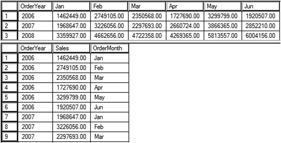
Figure 11-16. The partial results of UNPIVOT
You will unpivot the month columns, Jan through Jun. The SELECT part of the query contains any regular columns, in this case OrderYear. Next you list the name for the values in the columns to unpivot, Sales. The final column is the name of your unpivoted columns, Order Month. The list of columns is followed by the FROM clause containing a derived table, just the data to unpivot. The derived table must be aliased.
Now add the UNPIVOT function. The argument to the function contains a phrase consisting of the numeric column followed by FOR and the unpivot column. Then you must supply a hard-coded list of the columns. Finally, supply an alias. Figure 11-17 shows where OrderMonth and Sales originate.

Figure 11-17. The origination of the columns
Imaging that you are performing a search on your favorite e-commerce web site and several hundred products will be returned from your search. Instead of displaying all of the products at once, the site will display 10 or 20 products at a time. Hopefully, you will find what you need on the first or second page that is displayed and can complete the purchase.
The technique of displaying a page of data at a time is called paging. There are two ways that this is commonly done with T-SQL. The first method takes advantage of the ROW_NUMBER function. The second method uses the OFFSET/FETCH NEXT functionality added with SQL Server 2008.
To keep the following examples simple, assume that the data to be paged is static. Type in Listing 11-20 to learn these two techniques.
Listing 11-20. Paging with T-SQL
--1
DECLARE @PageSize INT = 5;
DECLARE @PageNo INT = 1;

;WITH Products AS(
    SELECT ProductID, P.Name, Color, Size,
        ROW_NUMBER() OVER(ORDER BY P.Name, Color, Size) AS RowNum
    FROM Production.Product AS P
    JOIN Production.ProductSubcategory AS S
        ON P.ProductSubcategoryID = S.ProductSubcategoryID
        JOIN Production.ProductCategory AS C
            ON S.ProductCategoryID = C.ProductCategoryID
        WHERE C.Name = 'Bikes'
)
SELECT TOP(@PageSize) ProductID, Name, Color, Size
FROM Products
WHERE RowNum BETWEEN (@PageNo -1) * @PageSize + 1
    AND @PageNo * @PageSize
ORDER BY Name, Color, Size;

--2
SELECT ProductID, P.Name, Color, Size
FROM Production.Product AS P
JOIN Production.ProductSubcategory AS S
    ON P.ProductSubcategoryID = S.ProductSubcategoryID
JOIN Production.ProductCategory AS C
    ON S.ProductCategoryID = C.ProductCategoryID
WHERE C.Name = 'Bikes'
ORDER BY P.Name, Color, Size
    OFFSET @PageSize * (@PageNo -1) ROWS FETCH NEXT @PageSize ROWS ONLY;
Figure 11-18 shows the results. Query 1 uses a CTE so that it can filter on the RowNum column. The TOP expression is used to control how many rows are returned. In this case, the @PageSize variable is used. In this example, five rows are returned per page and the first page is returned. When substituting the values for the variables in the WHERE clause expressions, rows 1 to 5 are returned.
(1 - 1) * 5 + 1 = Row 1
1 * 5 = Row 5
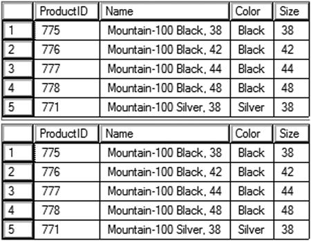
Figure 11-18. The paging results
Query 2 uses the newer syntax that is an enhancement of the ORDER BY clause. The value following the word OFFSET specifies how many rows to skip. The value following FETCH NEXT specifies how many rows to return. When substituting the values for the variables, 0 rows are skipped and 5 rows are returned.
5 * (1 – 1) = 0 Rows skipped
5 = 5 Rows to return
The OFFSET keyword can be used without FETCH NEXT. In that case, all possible rows after the offset are returned. Modify the values of the variables to perform additional tests of the two solutions.
Summary
This chapter covered how to write advanced queries using some T-SQL features supported in SQL Server. Starting with Chapter 6, you saw how CTEs can help you solve query problems without resorting to temporary tables or views. In this chapter, you learned several other ways to use CTEs, including how to display hierarchical data with a recursive CTE. With the OUTPUT clause, you can return or store the data involved in data manipulation statements. If you will be involved with loading data warehouses, you can use the MERGE and GROUPING SET, CUBE, and ROLLUP features. You learned two ways to write pivot queries, using CASE and using the PIVOT function. You also learned how to UNPIVOT data. Finally, you learned how to return data a page at a time.
Although the material in this chapter is not required knowledge for beginning T-SQL developers, it will be very beneficial to you to keep these techniques in mind. As you gain more experience, you will often find ways to take advantage of these features.
In Chapter 12 you will learn about T-SQL programming logic.