Balancing Your Checkbook

You will start by balancing your checkbook. This is the process by which you write down all your withdrawals and deposits and add them up. Then you try to figure out why you think you have $83,237.92 in the account while your bank lists the balance as $0.98.

Start the program LibreOffice Calc, or start LibreOffice and select New ➤ Spreadsheet. You’ll see a blank spreadsheet , as shown in Figure 5-1.

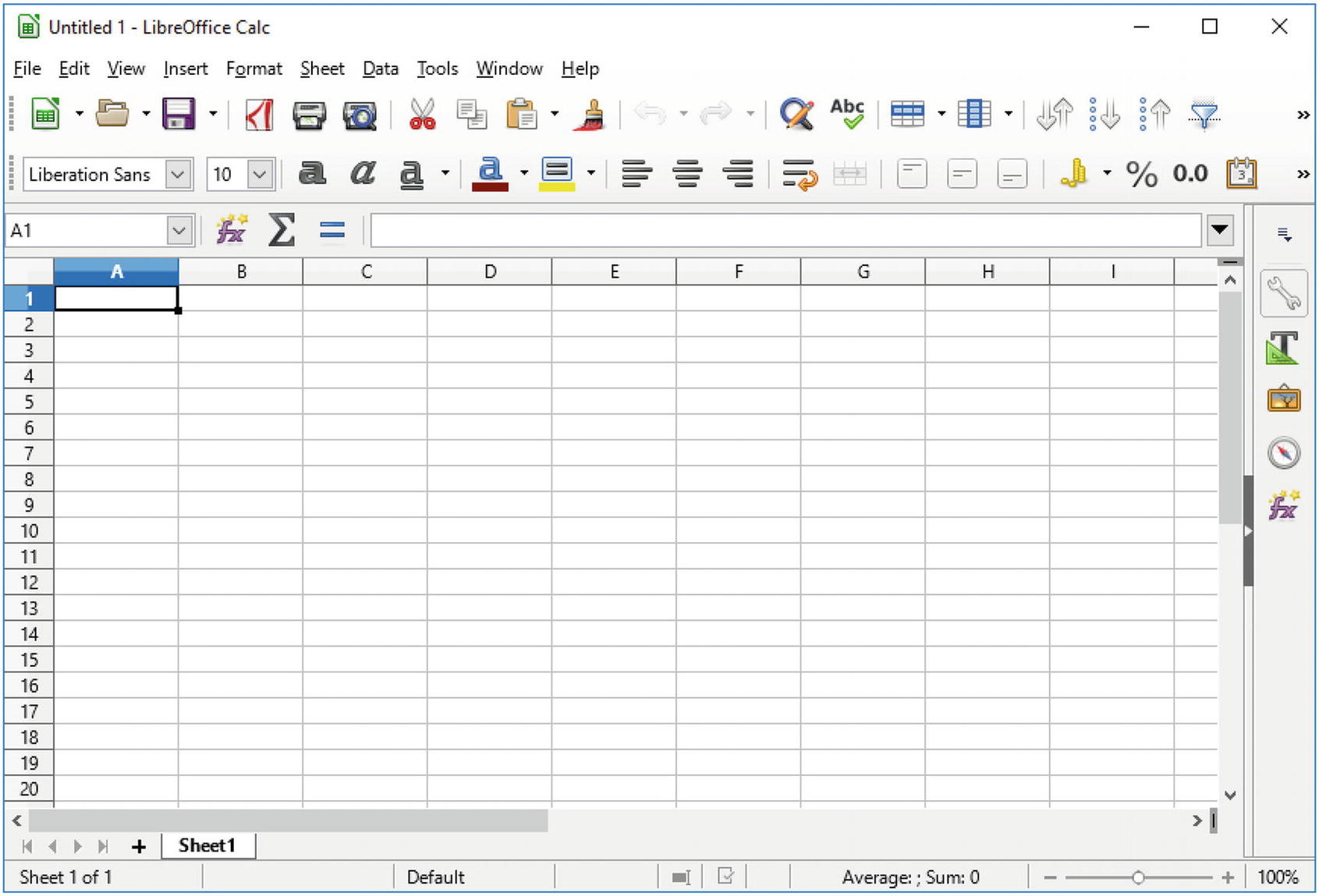
Figure 5-1 Initial Calc screen

You’ll notice that the program displays a grid of cells. The first cell is A1 in the upper-left corner, and then going across, they are A2, A3, A4, and so on. This will be important later.

You will want a set of headings for your checkbook, so let’s start by typing in the following:

• Date

• Check Number

• Description

• Amount

• Balance

After each entry, press Tab. Do not press Enter. If you make a mistake, just click in middle of a cell to start over in that cell. The result should look something like Figure 5-2.

Figure 5-2 Headings entered

You’ll notice that things are getting a little crowded, especially in the Check Number column. Let’s spread things out a little. Place the cursor on the line between the C and D columns and drag the line to the right to give you more room for the description. Now do the same for the check number.

Figure 5-3 shows the result .

Figure 5-3 Spreadsheet after column adjustments

Now let’s give the headings a little “oomph.” Click 1 on the left side to select the row and click the Bold icon to turn the text bold. Figure 5-4 shows the nicer-looking headings.

Figure 5-4 Bold headings

Next, let’s enter some data. Click in C2 and enter Initial balance. Now go to E2 and enter what’s in the bank, 1234.50. As you can see in Figure 5-5, something does not look right in cell E2. You are missing the 0 at the end.

Figure 5-5 Initial balance: funny money

The program thinks you are dealing with simple numbers and is displaying .50 as .5. People usually want to use two decimal points when working with money, so you need to change the way Calc formats the cells. You will do this for both columns D and E since both contain money. Click the D in the column headings and then Shift+click E. Both should be selected, as shown in Figure 5-6.

Now right-click and select Format Cells .

Figure 5-6 Formatting the row

This opens the Format Cells dialog, as shown in Figure 5-7.

Figure 5-7 Formatting cells

In the Category column, select Currency. The Format pull-down allows you to select different currency symbols . The default for this installation is the U.S. dollar ($), so leave that alone. (Your installation may have a different default depending on your Locale settings.) Let’s keep the format simple, so select -$1,234.00. This displays the dollars and cents and uses a minus (-) sign to indicate negative.

Click OK to format the cells. Now let’s enter some data, as shown here:

Figure 5-8 shows the result after typing =E2+D3 and just before pressing Enter.

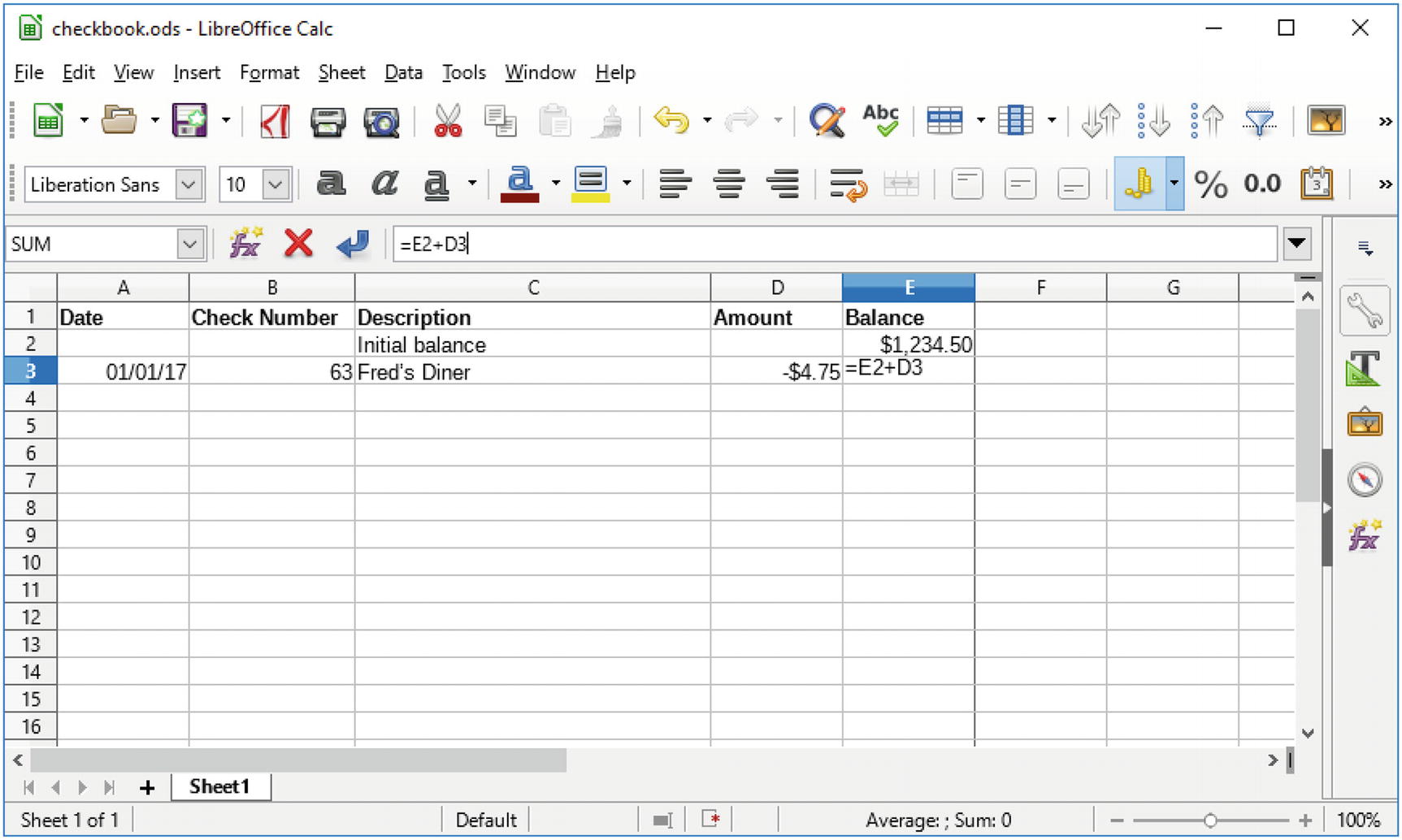
Figure 5-8 Your first check

Now press Enter to register the contents of your last cell. Notice that the contents change the value of the calculation. If you click the cell, you’ll see the original formula in the input line at the top of the sheet.

You’ll also notice that although you entered 1/1/2017, the spreadsheet reformatted it to 01/01/17. You can change this by changing the format of this column to another date format .

The check number 0063 got changed as well. Formatting won’t help this problem. Instead, you need to tell LibreOffice that this text is not a number. Let’s go back to that cell and enter a single quote mark (’) and the number. This is what it looks like:

'0063

There are two key characters that LibreOffice Calc looks for at the beginning of any entry. The first is a single quote, which indicates text. The second is an equal (=) sign, which indicates a formula. Anything else causes LibreOffice to guess at the type of data that’s being entered.

Figure 5-9 shows the result of the fixes.

Figure 5-9 Corrected entries

Now’s let’s add a new check to the spreadsheet, as shown in Figure 5-10.

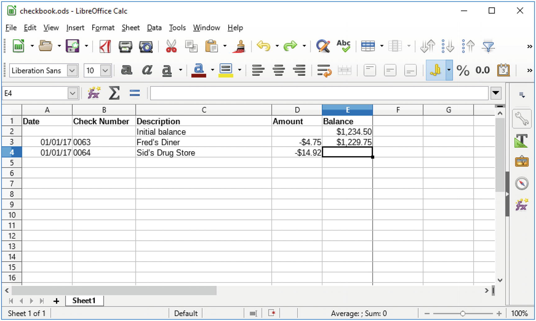
Figure 5-10 Second check

After entering the information shown in Figure 5-10, put the cursor in E3 and select Edit ➤ Copy. (Or press Ctrl+C.) Now put the cursor in E4 and select Edit ➤ Paste (or press Ctrl+V). The result is that a new balance is computed, as shown in Figure 5-11.

Figure 5-11 New balance

Notice that in the input bar the formula has been adjusted. Now all you have to do is repeat the process each time a check is written or a deposit is made, and you have yourself an automatic checkbook.

Creating a Double-Entry Checkbook

A classic ledger system has two entry columns, one for deposits and one for withdrawals. Let’s change your checkbook spreadsheet to handle these two types of entries.

Let’s start by adding a column for deposits. Right-click the Amount column and select Insert Column Left, as shown in Figure 5-12.

Figure 5-12 Inserting a column for deposits

Now you have a new column. Change the heading of the new column to Deposit and the old one, currently marked Amount, to Withdrawal. The result should look like Figure 5-13.

Figure 5-13 New column headings

Change the format of the new column (Deposit) to money like you did with the other money columns.

Change the amounts in cells E3 and E4 to positive numbers. Specifically, change the formula in cell F3 to F2+D3-E3. In other words, the new balance (the current cell) equals the old balance (F2) + deposits (D3) – withdrawals (E3). Then copy the formula from F3 to F4.

Now let’s add a new line to the bottom because you just got a check in from your employer. For the date, let’s use 1/5/17. For the description, enter Pay and put 1000 in the Deposit column. Copy cell F4 and paste it into F5 to complete the line, and you get the spreadsheet in Figure 5-14.

Figure 5-14 Completed checkbook spreadsheet

Creating a Budget

In this section, you’ll create a simple budget in a spreadsheet. Actually, you will make an over-simplified budget. A full budget is a wonderfully complex thing that covers everything you could possibly spend money on. In this section, we’ll show you the concepts needed to make a budget and leave the details to you and whatever financial advice you can find through Google.

The basic idea of a budget is to show what income you have and what you are spending your money on. Ideally, the former is bigger than the latter. If not, you use the budget to make adjustments.

Creating a Basic Budget

Let’s start by creating a spreadsheet with some basic information in it. On the left you will have income. On the right you will have spending with some basic entries. Your basic spreadsheet will look like Figure 5-15.

Note

At this time, we have not filled in any of the cells containing formulas.

Figure 5-15 Basic budget

Let’s start by cleaning up the headings. The Income section covers columns A and B. Let’s get the heading to cover these columns as well. First click cell A1, then Shift+click A2, and finally select Merge Cells , as shown in Figure 5-16.

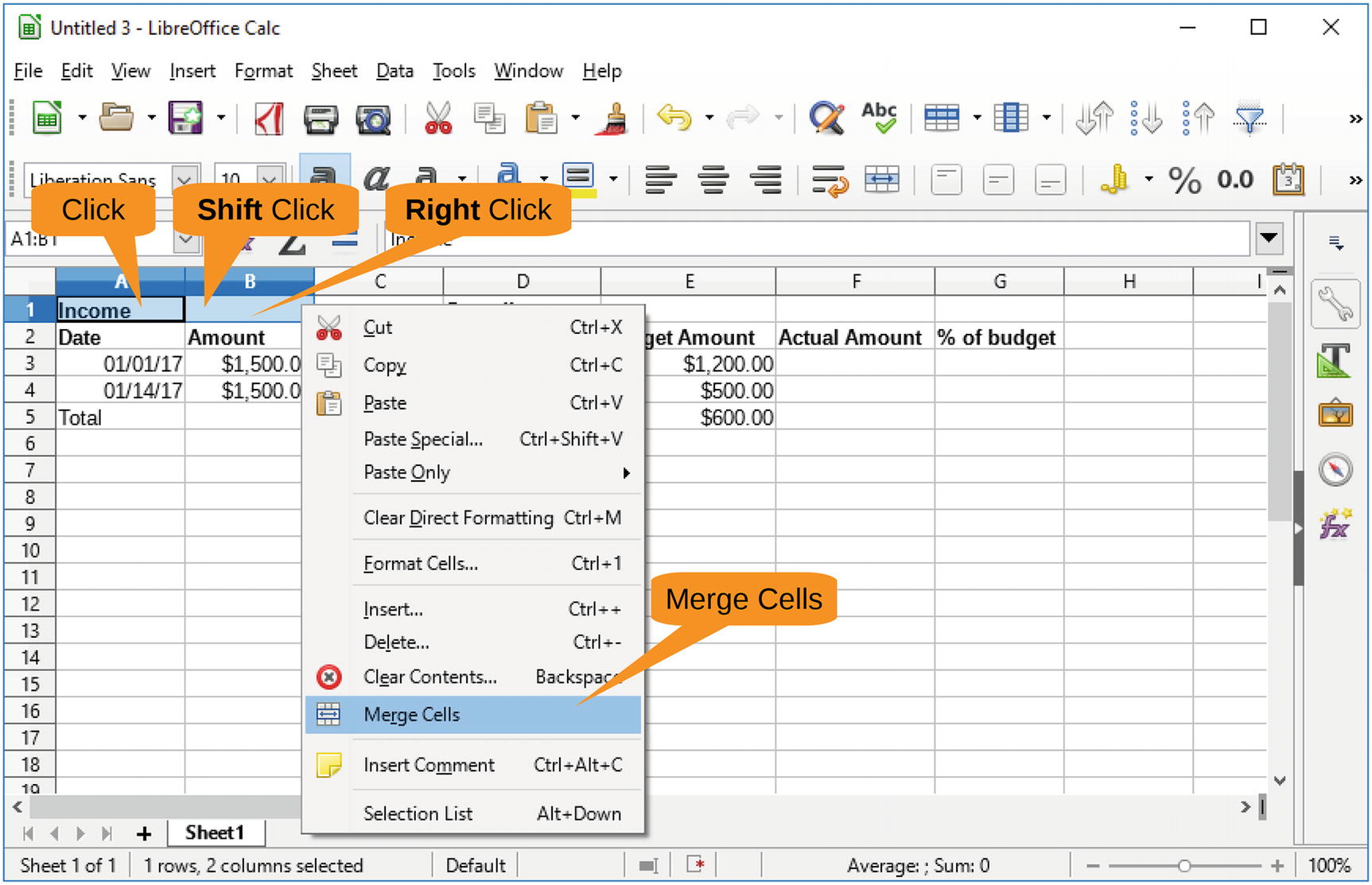
Figure 5-16 Merging cells

Let’s center the text by clicking cell A1 (or should we call it AB1?) and clicking the Center icon in the toolbar.

Now let’s do the same thing to the Spending cell. Click D1, Shift+click G1, right-click, and select Merge Cells. Now center this text.

While you are at it, let’s change the background to light yellow to make the section headings stand out. You can do this by clicking the Background Color icon. You now have a spreadsheet that looks something like Figure 5-17.

Figure 5-17 Spreadsheet with headings

Computing Totals

It’s time to compute some totals. You can get the total income by clicking cell B5 and clicking the Sum icon on the toolbar. LibreOffice will make an intelligent guess at what you want to add up. In this case, it thinks you want to add the column starting with B3 and ending with B4, so it fills in the formula as =SUM(B3:B4). It also draws a line around the cells it is going to sum up to give you a visual indication of what’s happening, as shown in Figure 5-18.

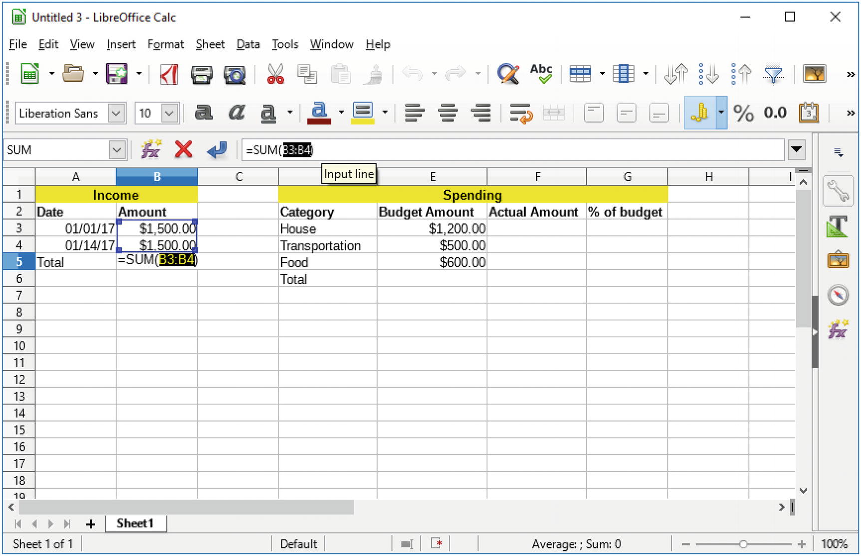
Figure 5-18 Summing up

Press Enter to accept this guess.

Now let’s add sums to the spending columns (actual and budgeted ). Figure 5-19 shows the result that includes the entry of some actual numbers.

Figure 5-19 Budget with totals

Now let’s see how well you stuck to your budget. Click cell G3 and enter the formula for the percent spent. That is, enter =E3/D3. The answer is 1. But you want a percentage. So, click the G3 cell to select it again, and click the “percent” symbol to turn the number into a percentage (100%), as shown in Figure 5-20.

Figure 5-20 Percentage

Copy and paste the formula from G3 into G4, G5, and G6. Uh-oh, you’re over budget. Figure 5-21 shows the damage.

It looks like one problem area is food, so to meet your budget for next month, all you have to do is stop eating…or maybe stop eating out so much.

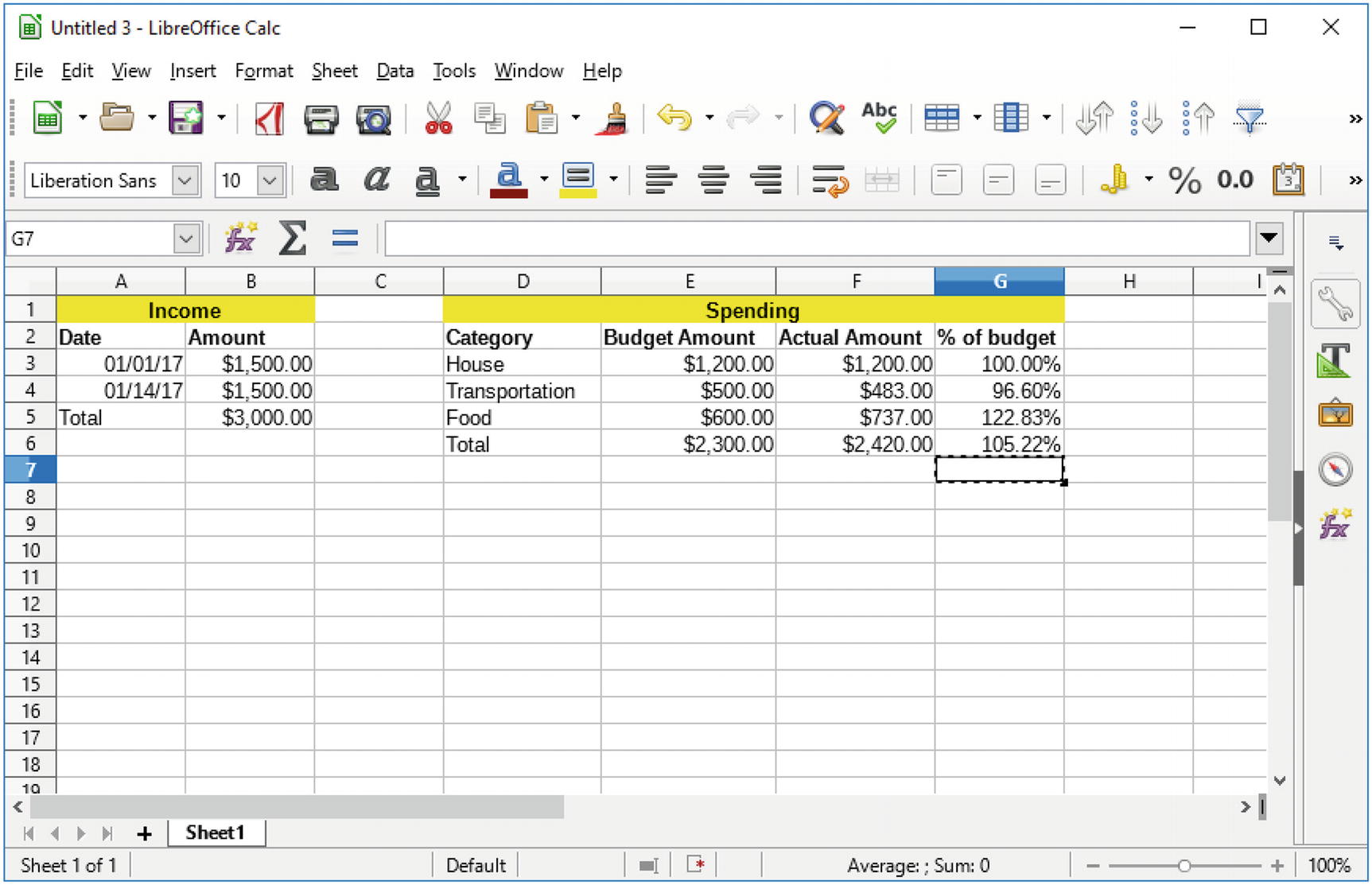
Figure 5-21 Final single-month budget

So far, we’ve covered just the month of January. What about next month and beyond? Let’s work on it.

Setting Up Multiple Sheets

Spreadsheets have a concept of multiple pages or sheets. So far, you have only one sheet, called imaginatively Sheet1. Let’s rename it to Jan17 and then copy it to a Feb17 sheet.

Right-click the sheet tab and select Rename Sheet , as demonstrated in Figure 5-22.

Figure 5-22 Renaming a sheet

The Rename Sheet dialog appears, as shown in Figure 5-23. Enter Jan17 and click OK to rename the sheet.

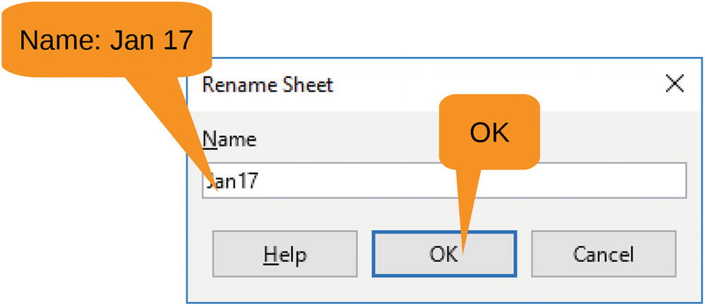
Figure 5-23 Rename Sheet dialog

Notice that the sheet name on the bottom tab is different. Now right-click the tab again, and as shown in Figure 5-24, select Move or Copy Sheet .

Figure 5-24 Getting ready to copy the sheet

The Move/Copy Sheet dialog appears, as shown in Figure 5-25. In this case, Copy is already selected for you. (It’s hard to change the sheet order in a one-sheet spreadsheet, so the Copy choice is forced upon you.) The document you want to copy into is the current document, so do not change the “To document” setting. Leave the “Insert before” setting at Jan17. You always want your newest budget to appear on top. Change the name to Feb17 and click OK.

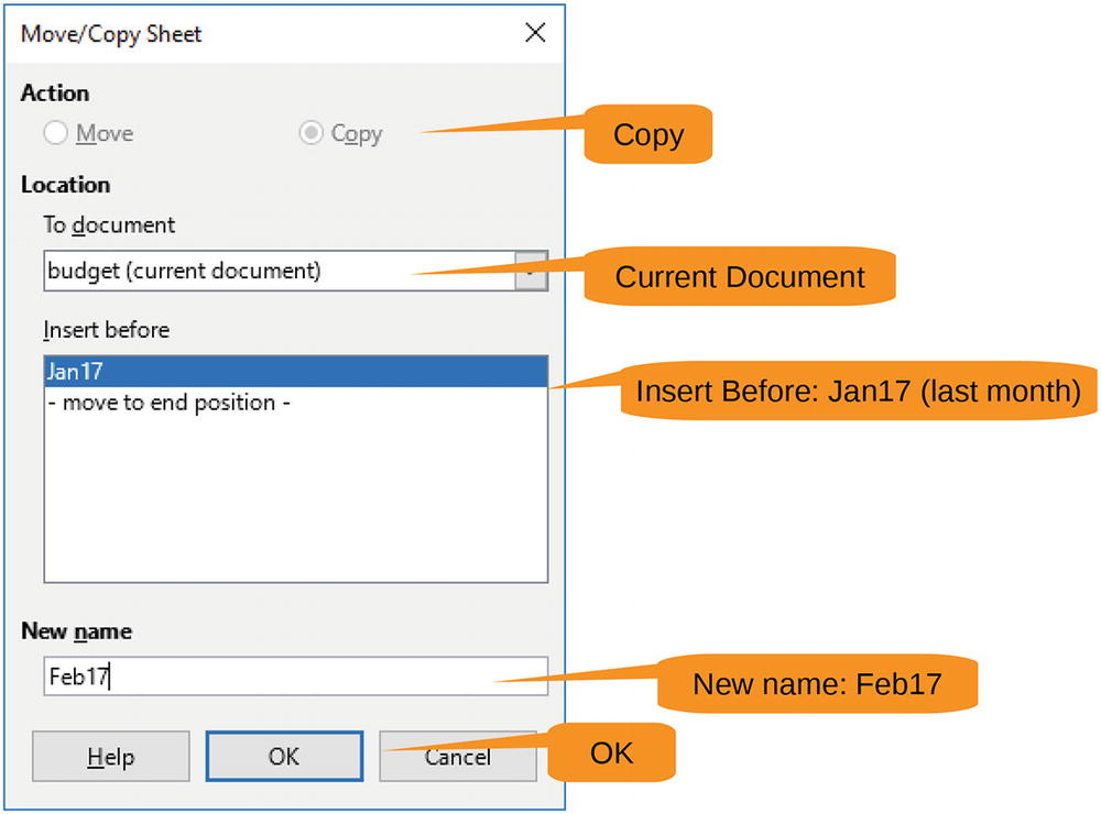
Figure 5-25 Move/Copy Sheet dialog

The new sheet, Feb17, appears on top. Now let’s fill in the numbers for February . Since it is a short month, you spent less, so you can be proud of the numbers in Figure 5-26.

Figure 5-26 February’s numbers

Now let’s add a section in which you reference last month’s numbers. Figure 5-27 shows the spreadsheet after entering the headings and the row label for Jan17. Note you have to put a single quote at the beginning of Jan17; otherwise, LibreOffice will think it’s a date and format at as 1/1/17.

Under Spent (cell B9), type = and nothing else.

Figure 5-27 Starting to reference previous months

Now you need to get the value of the total spent from Jan17. But it’s not a cell on the current sheet, so there is no A1, B2 type reference that you can use. But LibreOffice will fill in the cell reference automatically for you.

Click Jan17 to go to the Jan17 sheet and then click the F6 cell to select the total. Notice that the input bar now reads =Jan17.F6 and the cell is bordered with a purple rectangle. See Figure 5-28 for details.

Figure 5-28 Referencing the Jan17 value

No go back to the original sheet (Feb17) and press Enter. The value of that cell is automatically filled in. You can repeat this for the “% Budget” value as well.

Now all you need to do is create a “Feb 2017” line below the “Jan 2017” line and you have section giving you a two-month comparison of your spending. Figure 5-29 displays the final result.

Figure 5-29 Two months budgeted

Creating Charts

Now let’s insert a chart. There’s no good reason for inserting a chart in this budget, but we haven’t demonstrated the graphics features of LibreOffice Calc yet, so why not? First select cells D3 through D5 by clicking D3 and then Shift+clicking D5. Now let’s select cells F3 to F5 by Ctrl+clicking each of the three cells. Finally, as shown in Figure 5-30, you select Insert ➤ Chart.

Figure 5-30 Starting to insert a chart

The Chart Wizard shown in Figure 5-31 appears. Under Choose a Chart Type, select Pie and then click Finish.

Figure 5-31 Chart Wizard

Note that LibreOffice Calc has a complex charting system with hundreds of options. Going through them all would take another book. We’re after a quick-and-dirty chart, so we’re taking a lot of the defaults here.

After clicking Finish, the chart is inserted. Figure 5-32 shows you that the default location is right over your important data. So, you need to use the cursor to grab the edge of the chart and move it down.

Figure 5-32 Chart inserted

Dragging the chart down exposes all those lovely numbers that you worked so hard to come up, as shown in Figure 5-33. It also shows that we are paying far too much for housing, which should be no more than one-third of the budget. But that’s what we get for residing in such a grand fictional house . We probably should adjust our imagination and move into a less expensive home.

Figure 5-33 Final budget

Summary

LibreOffice Calc provides a full-featured spreadsheet. In this chapter, we covered the basic concepts that you’ll encounter in most simple spreadsheets. As you can see, LibreOffice Calc has all the useful features of the more expensive, proprietary spreadsheets but without the cost (and without the advertising budget).