Chapter 10. Real-Time Machine Learning
In the previous chapters, we ingested historical flight data and used it to train a machine learning model capable of predicting whether a flight will be late. We deployed the trained model and demonstrated that we could get the prediction for an individual flight by sending input variables to the model in the form of a REST call.
The input variables to the model include information about the flight whose on-time performance is desired. Most of these variables—the departure delay of the flight, the distance of the flight, and the time it takes to taxi out to the runway—are specific to the flight itself. However, the inputs to the machine learning model also included two time aggregates—the historic departure delay at the specific departure airport and the current arrival delay at the flight’s destination—that require more effort to compute. In Chapter 8, we wrote an Apache Beam pipeline to compute these averages on the training dataset so as to be able to train the machine learning model. In Chapter 9, we trained a TensorFlow model capable of using the input variables to predict whether the flight would be late. We were also able to deploy this model on Google Cloud Platform as a web service and invoke the service to make predictions.
In this chapter, we build a real-time Beam pipeline that takes each flight and adds the predicted on-time performance of the flight and writes it out to a database. The resulting table can then be queried by user-facing applications that need to provide information to users of the system interested in their specific flight. Although we could do prediction on behalf of individual users of their service as and when they request the status of their specific flight, this will probably end up being wasteful. It is far more efficient1 to compute the on-time arrival probability once, at flight takeoff, and then simply look up the flight information as required for specific users. It is worth noting that we are making predictions for a flight only at the time of takeoff (and not updating it as the flight is en route) because we trained our machine learning model only on flight data at the time of takeoff.
The advantage of using Apache Beam to compute time averages is that the programming model is the same for both historical data and for real-time data. Therefore, we will be able to reuse most of our training pipeline code in real time. The only changes we will need to make to the pipeline from Chapter 8 (that created the training dataset) are to the input (to read from Pub/Sub) and the output (to add predicted probability instead of the known on-time performance). To add the predicted probability, though, we need to invoke the trained TensorFlow model. Let’s write the code to do that first.
Invoking Prediction Service
In Chapter 9, we used Cloud AI Platform to deploy the trained TensorFlow model as a web service. We demonstrated that we could invoke the model by sending it a correctly formatted JSON request. For example, this JSON request2
{"instances":[{
"dep_delay":16.0,
"taxiout":13.0,
"distance":160.0,
"avg_dep_delay":13.34,
"avg_arr_delay":67.0,
"dep_lat":61.17,
"dep_lon":-150.0,
"arr_lat":60.49,
"arr_lon":-145.48,
"carrier":"AS",
"origin":"ANC",
"dest":"CDV"
}]}
yields this JSON response:
{'predictions': [{'pred': [0.7187997698783875]}]}
Recall that we trained the model to predict the probability of on-time arrival where we defined “on time” during training as an arrival delay of less than 15 minutes. Therefore, in this case, we are predicting that there is a 71.8% probability that the flight will have an arrival delay of less than 15 minutes. Because our threshold for canceling the meeting is that this probability is less than 70%, the recommendation will be to keep the meeting.
In Chapter 9, we demonstrated the call and response using Python, but because this is a REST web service, it can be invoked from pretty much any programming language as long as we can formulate the JSON, authenticate to Google Cloud Platform, and send an HTTP request. Let’s look at these three steps from our real-time pipeline.
Java Classes for Request and Response
To invoke the REST API from our Beam Java pipeline,3 we need to formulate and parse JSON messages in our Java program. A good way to do this is to represent the JSON request and response as Java classes (let’s call them Request and Response) and then use a library such as Jackson or GSON to do the marshaling from JSON and unmarshaling into JSON.
Based on the previous JSON example, the Request class definition is as follows:4
class Request {
    List<Instance> instances = new ArrayList<>();
}
class Instance {
    double dep_delay, taxiout, distance, avg_dep_delay, avg_arr_delay,
           dep_lat, dep_lon, arr_lat, arr_lon;
    String carrier, origin, dest;
 }
Note how arrays in JSON ([…]) are represented as a java.util.List and dictionaries ({…}) are represented as Java classes with appropriately named fields. Similarly, based on the example JSON response, the Response class definition is as follows:
class Response {
    List<Prediction> predictions = new ArrayList<>();
}
class Prediction {
    List<Double> pred = new ArrayList<>();
}
Creating a JSON request involves creating the Request object and using the GSON library to create the JSON representation:
Request req = …
Gson gson = new GsonBuilder().create();
String json = gson.toJson(req, Request.class);
We also can accomplish unmarshaling a JSON stream to a Response object from which we can obtain the predictions by using the same library:
String response = … // invoke web service
Response response = gson.fromJson(response, Response.class);
We don’t want to pollute the rest of our code with these Request and Response classes. So, let’s add a way to create a Request from a Flight object and a way to extract the probability of interest from a Response object. Every Flight corresponds to an Instance sent to the web service, so we will write a constructor that sets all the fields of the Instance object from the provided Flight:
 Instance(Flight f) {
      this.dep_delay = f.getFieldAsFloat(Flight.INPUTCOLS.DEP_DELAY);
      // etc.
      this.avg_dep_delay = f.avgDepartureDelay;
      this.avg_arr_delay = f.avgDepartureDelay;
      // etc.
      this.dest = f.getField(Flight.INPUTCOLS.DEST);
}
A Response consists of a list of predictions, one for each flight sent in the Request, so we will write an appropriate method in the Response class to pull out the probability that the flight is on time. The method will return an array of probabilities:
public double[] getOntimeProbability() {
      double[] result = new double[predictions.size()];
      for (int i=0; i < result.length; ++i) {
        Prediction pred = predictions.get(i);
        result[i] = pred.probabilities.get(1);
      }
      return result;
}
Post Request and Parse Response
Now that we have a way to create and parse JSON bytes, we are ready to interact with the Flights Machine Learning service. The service is deployed at this URL:
String endpoint = "https://ml.googleapis.com/v1/projects/"
       + String.format("%s/models/%s/versions/%s:predict",
                        PROJECT, MODEL, VERSION);
GenericUrl url = new GenericUrl(endpoint);
The code to authenticate to Google Cloud Platform, send the request, and get back the response is quite straightforward. We create an https transport and then send JSON bytes using HTTP POST. Here’s the response we get back:
GoogleCredential credential = // authenticate
                GoogleCredential.getApplicationDefault();
HttpTransport httpTransport = // https
                GoogleNetHttpTransport.newTrustedTransport();
HttpRequestFactory requestFactory =
                httpTransport.createRequestFactory(credential);
HttpContent content = new ByteArrayContent("application/json",
                json.getBytes()); // json
HttpRequest request = requestFactory.buildRequest("POST",
                url, content); // POST request
request.setUnsuccessfulResponseHandler(
                new HttpBackOffUnsuccessfulResponseHandler(
                     new ExponentialBackOff())); // fault-tol
request.setReadTimeout(5 * 60 * 1000); // 5 minutes
String response = request.execute().parseAsString(); // resp
Note that I have added in two bits of fault tolerance: if there is a network interruption or some temporary glitch (a non-2xx error from HTTP), I retry the request, increasing the time between retries using the ExponentialBackoff class. As of this writing, I observed that a sudden spike in traffic resulted in a 100- to 150-second delay as extra servers came online, hence the need for a longer-than-usual timeout.
Client of Prediction Service
The previous code example is wrapped into a helper class (FlightsMLService) that we can use to obtain the probability of a flight being on time:
public static double predictOntimeProbability(Flight f, double defaultValue)
throws IOException, GeneralSecurityException {
    if (f.isNotCancelled() && f.isNotDiverted()) {
      Request request = new Request();

      // fill in actual values
      Instance instance = new Instance(f);
      request.instances.add(instance);

      // send request
      Response resp = sendRequest(request);
      double[] result = resp.getOntimeProbability(defaultValue);
      if (result.length > 0) {
        return result[0];
      } else {
        return defaultValue;
      }
    }
    return defaultValue;
  }
Note that we check that the flight is not canceled or diverted—this is important because we trained the neural network only on flights with actual arrival information.
Adding Predictions to Flight Information
With the client to the Flights Machine Learning service in place, we can now create a pipeline that will ingest raw flight information at the time that a flight is taking off and invoke the prediction service. The resulting probability that the flight will be on time will be added to the flight information. Finally, both the original information about the flight and the newly computed probability will be saved.
In real time, this pipeline will need to listen to messages about flights coming in from Google Cloud Pub/Sub (recall that we set up a simulation to create this feed in Chapter 4) and stream the results into a durable, queryable store such as BigQuery.
Batch Input and Output
Before we do things in real time, though, let’s write a batch pipeline to accomplish the same thing. After the pipeline is working correctly, we can swap out the input and output parts to have the code work on real-time, streaming data (something Apache Beam’s unified batch/streaming model makes quite straightforward). Because we plan to swap the input and output, let’s capture that in a Java interface:5
interface InputOutput extends Serializable {
public PCollection<Flight> readFlights(Pipeline p, MyOptions options);
    public void writeFlights(PCollection<Flight> outFlights, MyOptions options);
}
The implementation for batch data reads from a BigQuery table and writes to text files on Google Cloud Storage. The reading code is similar to the code used in CreateTrainingDataset. The difference is that we read all flights, not just the ones that are not canceled or diverted. This is because we would like to store all the flight information that is sent to us in real time regardless of whether we can predict anything about that flight. Table 10-1 shows the crucial bits of code (with the Java boilerplate taken out).
| Step | What it does | Code |
|---|---|---|
| 1 | Create query |
String query = "SELECT EVENT_DATA FROM" + " flights.simevents WHERE " + " STRING(FL_DATE) = '2015-01-04' AND " + " (EVENT = 'wheelsoff' OR EVENT = 'arrived') "; |
| 2 | Read lines |
BigQueryIO.Read.fromQuery(query) |
| 3 | Parse into Flight object |
TableRow row = c.element();
String line = (String)
             row.getOrDefault("EVENT_DATA", "");
Flight f = Flight.fromCsv(line);
if (f != null) {
   c.outputWithTimestamp(f, f.getEventTimestamp());
}
|
When it comes to writing, we need to write out all the flight information that we receive. However, we also need to carry out prediction and write out the predicted probability. Let’s create an object to represent the data (flights + on-time probability) that we need to write out:
@DefaultCoder(AvroCoder.class)
public class FlightPred {
    Flight flight;
    double ontime;
    // constructor, etc.
}
The ontime field will hold the following:
-
The predicted on-time probability if the received event is
wheelsoff -
The actual on-time performance (0 or 1) if the received event is
arrived -
Null (however it is represented in the output sink) if the flight is canceled or diverted
The writing code then involves taking the flight information, adding the value of the ontime field, and writing it out:
PCollection<FlightPred> prds = addPrediction(outFlights);
PCollection<String> lines = predToCsv(prds);
lines.apply("Write", TextIO.Write.to(
     options.getOutput() + "flightPreds").withSuffix(".csv"));
The addPrediction() method is a ParDo.apply() of a DoFn whose processElement() method is:
 Flight f = c.element();
double ontime = -5;
if (f.isNotCancelled() && f.isNotDiverted()) {
if (f.getField(INPUTCOLS.EVENT).equals("arrived")) {
    // actual ontime performance
    ontime = f.getFieldAsFloat(INPUTCOLS.ARR_DELAY, 0) < 15 ? 1 : 0;
  } else {
    // wheelsoff: predict ontime arrival probability
    ontime = FlightsMLService.predictOntimeProbability(f, -5.0);
  }
}
c.output(new FlightPred(f, ontime));
When converting a FlightPred to a comma-separated value (CSV) file, we take care to replace the invalid negative value by null:
FlightPred pred = c.element();
String csv = String.join(",", pred.flight.getFields());
if (pred.ontime >= 0) {
  csv = csv + "," + new DecimalFormat("0.00").format(pred.ontime);
} else {
  csv = csv + ","; // empty string -> null
}
c.output(csv);
Data Processing Pipeline
Now that we have the input and output pieces of the pipeline implemented, let’s implement the middle of the pipeline. That part of the pipeline is the same as what was in CreateTrainingDataset (and in fact simply invokes those methods) except for the treatment of the departure delay:
    Pipeline p = Pipeline.create(options);
    InputOutput io = new BatchInputOutput();

    PCollection<Flight> allFlights = io.readFlights(p, options);

PCollectionView<Map<String, Double>> avgDepDelay =
readAverageDepartureDelay(p, options.getDelayPath());

    PCollection<Flight> hourlyFlights =
CreateTrainingDataset.applyTimeWindow(allFlights);

    PCollection<KV<String, Double>> avgArrDelay =
CreateTrainingDataset.computeAverageArrivalDelay(hourlyFlights);

hourlyFlights = CreateTrainingDataset.addDelayInformation(
hourlyFlights, avgDepDelay,
avgArrDelay, averagingFrequency);

   io.writeFlights(hourlyFlights, options);

    PipelineResult result = p.run();
    result.waitUntilFinish();
Whereas the arrival delay is computed over the current flights by the pipeline, the departure delay is simply read out of the global average (over the training dataset) that was written out during training:
private static PCollectionView<Map<String, Double>>
readAverageDepartureDelay(Pipeline p, String path) {
    return p.apply("Read delays.csv", TextIO.Read.from(path)) //
.apply("Parse delays.csv",
ParDo.of(new DoFn<String, KV<String, Double>>() {
     @ProcessElement
public void processElement(ProcessContext c) throws Exception {
            String line = c.element();
            String[] fields = line.split(",");
            c.output(KV.of(fields[0], Double.parseDouble(fields[1])));
          }
     })) //
        .apply("toView", View.asMap());
  }
The rest of the code is just like in CreateTrainingDataset. We get the average departure delay at the origin airport; apply an hourly sliding window; compute the average arrival delay over the previous hour at the destination airport; add the two delays to the flight data; and write out the flight information along with the predicted on-time performance.
Identifying Inefficiency
With the pipeline code written up, we can execute the batch pipeline on Google Cloud Platform in Cloud Dataflow. Unfortunately, when I did just that, I noticed that the inference kept failing. One way to monitor the usage of an API (our machine learning prediction is the Cloud ML Engine API) is from the API Dashboard part of the Google Cloud Platform web console. Looking at the traffic chart and breakdown of response codes in Figure 10-1, we immediately notice what is wrong.
The first few requests succeed with an HTTP response code of 200, but then the rest of the requests fail with a response code of 429 (“too many requests”). This pattern repeats—notice in Figure 10-1 the blue peaks of successful responses, followed by the much higher yellow peaks of failed responses.6 We could ask for a quota increase so that we can send more requests—from the graphs, it appears that we should request approximately five times the current quota.

Figure 10-1. Monitoring the usage of an API in the Google Cloud Platform web console
Before asking for a quota increase, however, we could look to see if we can optimize our pipeline to make fewer requests from the service.
Batching Requests
Whereas we do need to make predictions for each flight, we do not need to send the flight information to the service one-by-one. Instead of invoking the Flights Machine Learning service once for each flight, we could batch up requests. If we were to invoke the predictions for 60,000 flights into batches of 60 each, we’d be making only 1,000 requests. Making fewer requests will not only reduce costs, it might also end up increasing the overall performance by having less time spent waiting for a response from the service.
There are a couple of possible ways to batch up requests—based on count (accumulate flights until we reach a threshold, such as 100 flights, and invoke the service with these 100 flights) or based on time (accumulate flights for a fixed time span, such as two minutes, and invoke the service with all the flight information accumulated in that time period).
To batch requests based on count within a Cloud Dataflow pipeline, set up a trigger on a global window to operate on the count of records. This code will batch the inputs into groups of 100 each and ensure that the pipeline sends partial batches if waiting any further would cause the latency of the first element in the pane to go beyond one minute:
.apply(Window.into(new GlobalWindows()).triggering(
            Repeatedly.forever(AfterFirst.of(
                   AfterPane.elementCountAtLeast(100),
                   AfterProcessingTime.pastFirstElementInPane().
plusDelayOf(Duration.standardMinutes(1))))
In our case, however, we cannot do this. Recall that our pipeline does a sliding window (of one hour) in order to compute the average arrival delay and this average is part of the Flight object being written out. Applying a GlobalWindow later in the pipeline would cause the objects to be re-windowed so that any group-by-keys applied to the data afterward would happen globally—this is a side effect that we neither want nor need. Therefore, we should look for a batching method that operates in the context of a sliding window without doing its own Window.into().
Because we are already in the context of a sliding window, we could take all the flights that were used in the computation of the average delay, batch them, and get predictions for them. This is very appealing because we are obtaining the predicted on-time performance for a flight as soon as we have all the information that is needed in order to carry out machine learning interference—no additional delay is being introduced. Although we could combine all the flights over the past five minutes into a single batch and send it for inference, this will have the unwanted effect of being carried out on a single Cloud Dataflow worker. We should provide the ability to create a few batches from the flights over the five-minute period so that we can avoid overwhelming a single Cloud Dataflow worker node.
My solution to create a batch is to emit a key-value pair for each flight such that the key reflects the batch number of the flight in question:
Flight f = c.element();
String key = "batch=" + System.identityHashCode(f) % NUM_BATCHES;
c.output(KV.of(key, f));
We obtain the key by taking the identity hashcode of the object and finding the remainder when the hashcode is divided by NUM_BATCHES—this ensures that there are only NUM_BATCHES unique keys.7
To work within the context of a time-windowed pipeline, we follow the transform that emits key-value pairs (as we just did) with a GroupByKey:
PCollection<FlightPred> lines = outFlights //
     .apply("Batch->Flight", ParDo.of(...) // see previous fragment
     .apply("CreateBatches", GroupByKey.<String, Flight> create())
The GroupByKey will now output an Iterable<Flight> that can be sent along for prediction:
double[] batchPredict(Iterable<Flight> flights, float defaultValue) throws
IOException, GeneralSecurityException {
    Request request = new Request();
    for (Flight f : flights) {
      request.instances.add(new Instance(f));
    }
    Response resp = sendRequest(request);
    double[] result = resp.getOntimeProbability(defaultValue);
    return result;
  }
With this change, the number of requests drops dramatically, and is under quota, as demonstrated in Figure 10-2.

Figure 10-2. After the change to batch up requests, the number of requests drops significantly
Note how the same set of records is handled with far fewer requests after the change to send the requests in batches.
Streaming Pipeline
Now that we have a working data processing pipeline that can process bounded inputs, let’s change the input and output so that the pipeline works on streaming data. The pipeline will read from Cloud Pub/Sub and stream into BigQuery.
Flattening PCollections
When we read from text files, our data processing code received both arrived and wheelsoff events from the same text file. However, the simulation code that we wrote in Chapter 4 streams these events to two separate topics in Cloud Pub/Sub. To reuse the data processing code, we must ingest messages from both these topics and merge the two PCollections into one. We can accomplish merging PCollections of the same type by using the Flatten PTransform. The code, therefore, involves looping through the two events, creating two separate PCollections, and then invoking Flatten:
 // empty collection to start
 PCollectionList<Flight> pcs = PCollectionList.empty(p);
 // read flights from each of two topics
 for (String eventType : new String[]{"wheelsoff", "arrived"}){
String topic = "projects/" + options.getProject() +
"/topics/" + eventType;
    PCollection<Flight> flights = p.apply(eventType + ":read",
        PubsubIO.<String> read().topic(topic)
               .withCoder(StringUtf8Coder.of()) //
.timestampLabel("EventTimeStamp")) //
.apply(eventType + ":parse",
ParDo.of(new DoFn<String, Flight>() {
          @ProcessElement
public void processElement(ProcessContext c)
throws Exception {
            String line = c.element();
            Flight f = Flight.fromCsv(line);
            if (f != null) {
               c.output(f);
            }
          }
        }));
pcs = pcs.and(flights);
  }
  // flatten collection
  return pcs.apply(Flatten.<Flight>pCollections());
}
This is a pattern worth knowing—the way to create a pipeline from multiple sources is to ensure that you ingest each of the sources into PCollections of the same type, and then invoke the Flatten transform. The flattened collection is what will be processed by the rest of the pipeline.
Another thing to note is the presence of a timestampLabel in the PubsubIO read. Without the timestamp label, messages are assigned the timestamp at which the message was inserted into Pub/Sub. In most cases, this will suffice. However, I would like to use the actual time of the flight as the timestamp and not the time of insertion because I am simulating flight events at faster-than-real-time speeds. Being able to specify a timestamp label is also important in case there is latency between the creation of the message and its actual insertion into Pub/Sub. The timestampLabel refers to an attribute on the Pub/Sub message, and is specified by the publishing program:
def publish(topics, allevents, notify_time):
  timestamp = notify_time.strftime(RFC3339_TIME_FORMAT)
    for key in topics:  # 'departed', 'arrived', etc.
       topic = topics[key]
       events = allevents[key]
       with topic.batch() as batch:
          for event_data in events:
batch.publish(event_data, EventTimeStamp=timestamp)
Streaming the output FlightPred information to BigQuery involves creating TableRows and then writing to a BigQuery table:
String outputTable = options.getProject() + ':' + BQ_TABLE_NAME;
TableSchema schema = new TableSchema().setFields(getTableFields());
PCollection<FlightPred> preds = addPredictionInBatches(outFlights);
PCollection<TableRow> rows = toTableRows(preds);
rows.apply("flights:write_toBQ",BigQueryIO.Write.to(outputTable) //
    .withSchema(schema));
Executing Streaming Pipeline
Now that the pipeline code has been written, we can start the simulation from Chapter 4 to stream records into Cloud Pub/Sub:
cd ../04_streaming/simulate
python simulate.py --project <PROJECT-ID> --startTime "2015-04-01 00:00:00 UTC" -
-endTime "2015-04-03 00:00:00 UTC" --speedFactor 60
Then, we can start the Cloud Dataflow pipeline to consume these records, invoke the Flights ML service, and write the resulting records to BigQuery:
mvn compile exec:java
-Dexec.mainClass=com.google.cloud.training.flights.AddRealtimePrediction
 -Dexec.args="--realtime --speedupFactor=60 --maxNumWorkers=10 --
autoscalingAlgorithm=THROUGHPUT_BASED"
The realtime option allows us to switch the pipeline between the two implementations of InputOutput (batch and real time), and in this case, to use the Pub/Sub to BigQuery pipeline.
With the pipeline running, we can navigate over to the BigQuery console, shown in Figure 10-3, and verify that flight information is indeed being streamed in.

Figure 10-3. Streaming predictions of on-time arrival probability
The query in Figure 10-3 is looking at flights between Dallas/Fort Worth (DFW) and Denver (DEN) and ordering and limiting the result set so that the five latest flights are retained. We see that row 1 is an American Airlines (AA) flight that arrived on time in spite of a departure delay of 19 minutes. On row 4, we see the earlier prediction by the service for that flight at the time of wheels off, indicating that this was only 56% likely to happen.
Late and Out-of-Order Records
Our simulation uses the flight record time to add records into Cloud Pub/Sub in precise order. In real life, though, flight records are unlikely to arrive in order. Instead, network vagaries and latencies can cause late and out-of-order records. To simulate these essentially random effects, we should change our simulation to add a random delay to each record.
We can do this in the BigQuery SQL statement that is used by the simulation program to read in the flight records:
SELECT
  EVENT,
  NOTIFY_TIME AS ORIGINAL_NOTIFY_TIME,
  TIMESTAMP_ADD(NOTIFY_TIME, INTERVAL CAST (0.5 + RAND()*120 AS INT64) SECOND)
  AS NOTIFY_TIME, EVENT_DATA
FROM
  `flights.simevents`
Because RAND() returns a number that is uniformly distributed between 0 and 1, multiplying the result of RAND() by 120 yields a delay between 0 and 2 minutes.
Running this query on the BigQuery console, we notice that it works as intended—the records now reflect some jitter, as depicted in Figure 10-4.

Figure 10-4. Adding random jitter to the notification time
Note that the first record is delayed by one second, whereas the second record, which is nominally at the same time, is now six seconds later.
Uniformly distributed delay
A zero delay is highly unrealistic, however. We could change the formula to simulate other scenarios. For example, if we want to have latencies between 90 and 120 seconds, we would change the jitter to be CAST(90.5 + RAND()*30 AS INT64). The resulting distribution might look like Figure 10-5.

Figure 10-5. Uniformly distributed jitter
Even this strikes me as being unrealistic. I don’t know what the delay involved with the flight messages is,8 but there seem to be two possibilities: an exponential distribution and a normal distribution.
Exponential distribution
An exponential distribution is the theoretical distribution associated with the time between events during which the events themselves happen at a constant rate. If the network capacity is limited by the number of events, we’d observe that the delay follows an exponential distribution. To simulate this, we can create the jitter variable following this formula:
CAST(-LN(RAND()*0.99 + 0.01)*30 + 90.5 AS INT64)
The resulting distribution would look something like that shown in Figure 10-6.
With the exponential distribution, latencies of 90s are much more common than latencies of 150s, but a few records will encounter unusually high latencies.

Figure 10-6. Exponential distribution of jitter: smaller values are much more likely than large values
Normal distribution
A third alternative distribution for the delay is that it follows the law of big numbers, and that if we observe enough flight events, we might observe that the delay is normally distributed around some mean with a certain standard deviation. Of course, the delay must be positive, so the distribution would be truncated at zero.
Generating a normally distributed random variable is difficult to do with just plain SQL. Fortunately, BigQuery allows for user-defined functions (UDFs) in JavaScript. This JavaScript function uses the Marsaglia polar rule to transform a pair of uniformly distributed random variables into one that is normally distributed:
js = """
    var u = 1 - Math.random();
    var v = 1 - Math.random();
    var f = Math.sqrt(-2 * Math.log(u)) * Math.cos(2*Math.PI*v);
    f = f * sigma + mu;
    if (f < 0)
       return 0;
    else
       return f;
""".replace('
', ' ')
We can use the preceding JavaScript to create a temporary UDF invokable from SQL:
sql = """
CREATE TEMPORARY FUNCTION
trunc_rand_normal(x FLOAT64, mu FLOAT64, sigma FLOAT64)
RETURNS FLOAT64
LANGUAGE js AS "{}";

SELECT
  trunc_rand_normal(ARR_DELAY, 90, 15) AS JITTER
FROM
  ...
""".format(js).replace('
', ' ')
The resulting distribution of jitter might look something like Figure 10-7 (the preceding code used a mean of 90 and a standard deviation of 15).

Figure 10-7. Normally distribution jitter, with a jitter of 90s most likely
To experiment with different types of jitter, let’s change our simulation code to add random jitter to the notify_time:9
jitter = 'CAST (-LN(RAND()*0.99 + 0.01)*30 + 90.5 AS INT64)'

# run the query to pull simulated events
querystr = """
SELECT
  EVENT,
TIMESTAMP_ADD(NOTIFY_TIME, INTERVAL {} SECOND) AS NOTIFY_TIME,
  EVENT_DATA
FROM
  `cloud-training-demos.flights.simevents`
WHERE
  NOTIFY_TIME >= TIMESTAMP('{}')
  AND NOTIFY_TIME < TIMESTAMP('{}')
ORDER BY
  NOTIFY_TIME ASC
"""
query = bqclient.run_sync_query(querystr.format(jitter,
                                                   args.startTime,
                                                   args.endTime))
Watermarks and Triggers
The Beam programming model implicitly handles out-of-order records within the sliding window, and by default accounts for late-arriving records. Beam employs the concept of a watermark, which is the oldest unprocessed record left in the pipeline. The watermark is an inherent property of any real-time data processing system and is indicative of the lag in the pipeline. Cloud Dataflow tracks and learns this lag over time.
If we are using the time that a record was inserted into Cloud Pub/Sub as the event time, the watermark is a strict guarantee that no data with an earlier event time will ever be observed by the pipeline. On the other hand, if the user specifies the event time (by specifying a timestampLabel), there is nothing to prevent the publishing program from inserting a really old record into Cloud Pub/Sub, and so the watermark is a learned heuristic based on the observed historical lag. The concept of a watermark is more general than Cloud Pub/Sub, of course—in the case of streaming sources (such as low-power Internet of Things devices) that are intermittent, watermarking helps those delays as well.
Computation of aggregate statistics is driven by a “trigger.” Whenever a trigger fires, the pipeline calculations are carried out. Our pipeline can include multiple triggers, but each of the triggers is usually keyed off the watermark. The default trigger is
Repeatedly.forever(AfterWatermark.pastEndOfWindow())
which means that the trigger fires when the watermark passes the end of the window and then immediately whenever any late data arrives. In other words, every late-arriving record is processed individually. This prioritizes correctness over performance.
What if we add a uniformly distributed jitter to the simulation? Because our uniform delay is in the range of 90 to 120, the actual difference in delay between the earliest-arriving and latest-arriving records is 30 seconds. So, Cloud Dataflow needs to keep windows open 30 seconds longer.
The Cloud Dataflow job monitoring web page on the Cloud Platform Console indicates the learned watermark value. We can click any of the transform steps to view what this value is. And with a uniform delay added to the simulation, the monitoring console (Figure 10-8) shows us that this is what is happening.

Figure 10-8. Although the simulation is sending events at 12 minutes and 32 seconds past the hour, the Dataflow pipeline shows a watermark at 11 minutes and 50 seconds past the hour, indicating that the time windows are being kept open about 42 seconds longer
We see that the simulation (righthand side of Figure 10-8) is sending events at 00:12:32 UTC, whereas the watermark shown by the monitoring console is at 17:11:50 Pacific Standard Time. Ignoring the seven hours due to time zone conversion, Cloud Dataflow is keeping windows open for 42 seconds longer (this includes the system lag of seven seconds, which is the time taken to process the records).
Unlike uniform jitter, small delays are far more likely than larger delays in exponentially distributed jitter. With exponentially distributed jitter added to the simulated data in the Cloud Pub/Sub pipeline, the learned watermark value is 21 seconds (see Figure 10-9).

Figure 10-9. Because small delays are more likely in exponentially distributed jitter, the window is being kept open only about 21 seconds longer
Recall that the default trigger prioritizes correctness over performance, processing each late-arriving record one by one and updating the computed aggregates. Fortunately, changing this trade-off is quite easy. Here is a different trade-off:
.triggering(Repeatedly.forever(
            AfterWatermark.pastEndOfWindow()
            .withLateFirings(
                AfterPane.elementCountAtLeast(10))
            .orFinally(AfterProcessingTime.pastFirstElementInPane()
                .plusDelayOf(Duration.standardMinutes(30)))))
Here, the calculations are triggered at the watermark (as before). Late records are processed 10 at a time but only if they arrive within 30 minutes after the start of the plane. Beyond that, late records are thrown away.
Transactions, Throughput, and Latency
Streaming the output flight records to BigQuery is acceptable for my flight delay scenario, but it might not be the right choice for your data pipeline. You should select the output sink based on four factors: access pattern, transactions, throughput, and latency.
If your primary access pattern is around long-term storage and delayed access to the data, you could simply stream to sharded files on Cloud Storage. Files on Cloud Storage can serve as staging for later import into Cloud SQL or BigQuery for later analysis of the data. In the rest of this section, I will assume that you will need to query the data in near real time.
Recall that we receive several events for each flight—departed, wheelsoff, and so on. Should we have a single row for each flight that reflects the most up-to-date state for that flight? Or can the data be append-only so that we simply keep storing flight events as they come streaming in? Is it acceptable for readers to possibly get slightly out-of-date records, or is it essential for there to be a single source of truth and consistent behavior throughout the system? The answers to these questions determine whether flight updates need to be transactional, or whether flight updates can be done in an environment that provides only eventual consistency guarantees.
How many flight events come in every second? Is this rate constant, or are there periods of peak activity? The answers here determine the throughput that the system needs to handle. If we are providing for eventual consistency, what is the acceptable latency? After flight data is added to the database, within what time period should all readers see the new data? As of this writing, streaming into BigQuery supports up to 100,000 events/second with latency on the order of a few seconds. For throughput needs that are higher, or latency requirements that are lower than this, we need to consider other solutions.
Possible Streaming Sinks
If transactions are not needed, and we simply need to append flight events as they come in, we can use BigQuery, text files, or Cloud Bigtable:
-
BigQuery is a fully managed data warehouse that supports SQL queries. Streaming flight events directly into BigQuery is useful for throughputs of tens of thousands of records per second and acceptable latencies of a few seconds. Many dashboard applications fall into this sweet spot.
-
Cloud Dataflow also supports streaming into text files on Cloud Storage. This is obviously useful if the primary use case is to simply save the data, not to analyze it. However, it is also a solution to consider if periodic batch updates into BigQuery will suffice. For example, we could stream into text files that are sharded by hour, and at the end of the hour, we could do a batch upload of the file into BigQuery. This is less expensive than streaming into BigQuery and can be used if hourly latencies are acceptable.
-
Cloud Bigtable is a massively scalable NoSQL database service—it can handle workloads that involve hundreds of petabytes with millions of reads and writes per second at a latency that is on the order of milliseconds. Moreover, the throughput that can be handled by Cloud Bigtable scales linearly with the number of nodes—for example, if a single node supports 10,000 reads or writes in six milliseconds, a Cloud Bigtable instance with 100 nodes will support a million reads or writes in the same 6-millisecond interval. In addition, Cloud Bigtable automatically rebalances the data to improve query performance and availability.
On the other hand, if transactions are needed and you want to have a single record that reflects the most current state of a flight, we could use a traditional relational database, a NoSQL transactional database, or Cloud Spanner:
-
Cloud SQL, which is backed by either MySQL or PostgreSQL, is useful for frequently updated, low-throughput, medium-scale data that you want to access from a variety of tools and programming languages in near real time. Because relational technologies are ubiquitous, the tools ecosystem tends to be strongest for traditional relational databases. For example, if you have third-party, industry-specific analysis tools, it is possible that relational databases might be the only storage mechanism to which they will connect. Before choosing a traditional relational database solution, though, consider whether the use case is such that you will run into throughput and scaling limitations.
-
You can scale to much larger datasets (terabytes of data) and avoid the problem of converting between hierarchical objects and flattened relational tables by using Cloud Datastore, which is a NoSQL object store. Cloud Datastore provides high throughput and scaling by designing for eventual consistency. However, it is possible to achieve strong (or immediate) consistency on queries that involve lookups by key or “ancestor queries” that involve entity groups. Within an entity group, you get transactions, strong consistency, and data locality. Thus, it is possible to balance the need for high throughput and many entities while still supporting strong consistency where it matters.
-
Cloud Spanner provides a strongly consistent, transactional, SQL-queryable database that is nevertheless globally available and can scale to extremely large amounts of data. Cloud Spanner offers latency on the order of milliseconds, has extremely high availability (downtimes of less than five minutes per year), and maintains transactional consistency and global reach. Cloud Spanner is also fully managed, without the need for manual intervention for replication or maintenance.
In our use case, we don’t need transactions. Our incoming stream has fewer than 1,000 events per second. A few seconds’ latency between insert into the database and availability to applications that need the flight delay information is quite tolerable, given that what we might do is to simply send alerts to our users if their flight is likely to be delayed. BigQuery is fully managed, supported by many data visualization and report-creation products, and relatively inexpensive compared to the alternative choices. Based on these considerations, streaming into BigQuery is the right choice for our use case.
Cloud Bigtable
However, just as a hypothetical scenario, what if our stream consisted of hundreds of thousands of flight events per second, and our use case required that the latency be on the order of milliseconds, not seconds? This would be the case if each aircraft provides up-to-the-minute coordinate information while it is en route, and if the use case involves traffic control of the air space. In such a case, Cloud Bigtable would be a better choice. Let’s look at how we’d build the pipeline to write to Cloud Bigtable if this were the case.
Cloud Bigtable separates compute and storage. Tables in Cloud Bigtable are sharded into blocks of contiguous rows, called tablets. The Cloud Bigtable instance doesn’t store these tablets; instead, it stores pointers to a set of tablets, as illustrated in Figure 10-10. The tablets themselves are durably stored on Cloud Storage. Because of this, a node can go down, but the data remains in Cloud Storage. Work might be rebalanced to a different node, and only metadata needs to be copied.

Figure 10-10. How storage in Cloud Bigtable is organized
The data itself consists of a sorted key-value map (each row has a single key). Unlike BigQuery, Cloud Bigtable’s storage is row-wise, and the rows are stored in sorted order of their key value. Columns that are related are grouped into a “column family,” with different column families typically managed by different applications. Within a column family, columns have unique names. A specific column value at a specific row can contain multiple cells at different timestamps (the table is append-only, so all of the values exist in the table). This way, we can maintain a time–series record of the value of that cell over time. For most purposes,10 Cloud Bigtable doesn’t care about the data type—all data is treated as raw byte strings.
The performance of Cloud Bigtable table is best understood in terms of the arrangement of rows within a tablet (blocks of contiguous rows into which tables in Cloud Bigtable are sharded). The rows are in sorted order of the keys. To optimize the write performance of Cloud Bigtable, we want to have multiple writes happening in parallel, so that each of the Cloud Bigtable instances is writing to its own set of tablets. This is possible if the row keys do not follow a predictable order. The read performance of Cloud Bigtable is, however, more efficient if multiple rows can be read at the same time. Striking the right balance between the two contradictory goals (of having writes be distributed while making most reads be concentrated) is at the heart of effective Cloud Bigtable schema design.
Designing Tables
At the extremes, there are two types of designs of tables in Cloud Bigtable. Short and wide tables take advantage of the sparsity of Cloud Bigtable, whereas tall and narrow tables take advantage of the ability to search row keys by range.
Short and wide tables use the presence or absence of a column to indicate whether or not there is data for that value. For example, suppose that we run an automobile factory and the primary query that we want to support with our dataset is to determine the attributes of the parts (part ID, supplier, manufacture location, etc.) that make up a specific automobile. Imagine that we will have millions of cars, each with hundreds of thousands of parts. We could use the car serial number as the row key and each unique part (e.g., a spark plug) could have a column associated with it, as demonstrated in Figure 10-11.

Figure 10-11. Designing a short and wide table in Cloud Bigtable
Each row then consists of many events, and is updated as the automobile is put together on the assembly line. Because cells that have no value take up no space, we don’t need to worry about the proliferation of columns over time as new car models are introduced. Because we will tend to receive events from automobiles being manufactured at the same time, we should ensure that automobile serial numbers are not consecutive, but instead start with the assembly line number. This way, the writes will happen on different tablets in parallel, and so the writes will be efficient. At the same time, diagnostic applications troubleshooting a quality issue will query for all vehicles made on the same line on a particular day, and will therefore tend to pull consecutive rows. Service centers might be interested in obtaining all the parts associated with a specific vehicle. Because the vehicle ID is the row key, this requires reading just a single row, and so the read performance of such a query will also be very efficient.
Tall and narrow tables often store just one event per row. Every flight event that comes in could be streamed to a new row in Cloud Bigtable. This way, we can have multiple states associated with each flight (departed, wheels-off, etc.) and the historical record of these. At the same time, for each flight, we have only 20 or so fields, all of which can be part of the same column family. This makes the streaming updates easy and intuitive.
Designing the Row Key
Although the table design of one row per event is very intuitive, we need to design the row key in a way that both writes and reads are efficient. To make the reads efficient, consider that the most common queries will involve recent flights between specific airports on a specific carrier (e.g., the status of today’s flight between SEA and SJC on AS). Using multiple rows, with a single version of an event in each row, is the simplest way to represent, understand, and query your data. Tall and narrow tables are most efficient if common queries involve just a scan range of rows. We can achieve this if the origin and destination airports are part of the key, as is the carrier. Thus, our row-key can begin with:
ORIGIN#DEST#CARRIER
Having the row key begin with these three fields also helps with optimizing write performance. Even though the tablets associated with busy airports like Atlanta might get some amount of hotspotting, the overload will be counteracted by the many sleepy airports whose names also begin with the letter A. An alphabetical list of airports should therefore help distribute the write load. Notice that I have the carrier at the end of the list—putting the carrier at the beginning of the row key will have the effect of overloading the tablets that contain the larger airlines (American and United); because there are only a dozen or so carriers, there is no chance of this load being counteracted by smaller carriers.
Because common queries will involve the latest data, scan performance will be improved if we could store the most current data at the “top” of the table. Using the timestamp in the most intuitive way
2017-04-12T13:12:45Z
will have the opposite effect. The latest data will be at the bottom of the table. Therefore, we need to store timestamps in reverse order somehow. One way would be to convert timestamps to the number of milliseconds since 1970, and then to compute the difference of that timestamp from the maximum possible long value:
LONG_MAX - millisecondsSinceEpoch
Where should the timestamp go? Having the timestamp at the beginning of the row key would cause the writing to become focused on just one tablet at a time. So, the timestamp needs to be at the end of the row key. In summary, then, our row key will be of the form:
ORIGIN#DEST#CARRIER#ReverseTimeStamp
But which timestamp? We’d like all of the events from a particular flight to have the same row key, so we’ll use the scheduled departure time in the key. This avoids problems associated with the key being different depending on the departure delay.
Streaming into Cloud Bigtable
We can create a Cloud Bigtable instance to stream flight events into by using gcloud:
gcloud bigtable
    instances create flights
    --cluster=datascienceongcp --cluster-zone=us-central1-b
    --description="Chapter 10" --instance-type=DEVELOPMENT
The name of my instance is flights, and the name of the cluster of machines is datascienceongcp.11 By choosing a development instance type, I get to limit the costs—the cluster itself is not replicated or globally available.
Within the Cloud Dataflow code, we refer to the instance in the context of the project ID:
private static String INSTANCE_ID = "flights";
private String getInstanceName(MyOptions options) {
  return String.format("projects/%s/instances/%s", options.getProject(),
  INSTANCE_ID);
}
On the Cloud Bigtable instance, we will create a table named predictions. In the code, it is referred to in the context of the instance (which itself incorporates the project ID):
private static String TABLE_ID = "predictions";
private String getTableName(MyOptions options) {
return String.format("%s/tables/%s", getInstanceName(options), TABLE_ID);
}
All of the columns will be part of the same column family, CF:
private static final String CF_FAMILY = "FL";
With this setup out of the way, we can create an empty table in the instance:
Table.Builder tableBuilder = Table.newBuilder();
ColumnFamily cf = ColumnFamily.newBuilder().build();
tableBuilder.putColumnFamilies(CF_FAMILY, cf);

BigtableSession session = new BigtableSession(optionsBuilder
.setCredentialOptions( CredentialOptions.credential(
options.as( GcpOptions.class
         ).getGcpCredential())).build()));

BigtableTableAdminClient tableAdminClient =
         session.getTableAdminClient();

CreateTableRequest.Builder createTableRequestBuilder = //
         CreateTableRequest.newBuilder() //
            .setParent(getInstanceName(options)) //
            .setTableId(TABLE_ID).setTable(tableBuilder.build());
tableAdminClient.createTable(createTableRequestBuilder.build());
The streaming Cloud Dataflow pipeline in the previous section had a PTransform that converts Flight objects into TableRow objects so as to be able to stream the information into BigQuery. To stream into Cloud Bigtable, we need to create a set of Cloud Bigtable mutations (each mutation consists of a change to a single cell):
PCollection<FlightPred> preds = ...;
BigtableOptions.Builder optionsBuilder = //
        new BigtableOptions.Builder()//
            .setProjectId(options.getProject()) //
            .setInstanceId(INSTANCE_ID)//
            .setUserAgent("datascience-on-gcp");
createEmptyTable(options, optionsBuilder);
PCollection<KV<ByteString, Iterable<Mutation>>> mutations =
toMutations(preds);
mutations.apply("write:cbt", //
BigtableIO.write() //
        .withBigtableOptions(optionsBuilder.build())//
        .withTableId(TABLE_ID));
The PTransform to convert flight predictions to mutations creates the row key from the flight information:
FlightPred pred = c.element();
String key = pred.flight.getField(INPUTCOLS.ORIGIN) //
    + "#" + pred.flight.getField(INPUTCOLS.DEST) //
    + "#" + pred.flight.getField(INPUTCOLS.CARRIER) //
    + "#" + (Long.MAX_VALUE - pred.flight.getFieldAsDateTime(
                      INPUTCOLS.CRS_DEP_TIME).getMillis());
For every column, a mutation is created
List<Mutation> mutations = new ArrayList<>();
long ts = pred.flight.getEventTimestamp().getMillis();
for (INPUTCOLS col : INPUTCOLS.values()) {
addCell(mutations, col.name(), pred.flight.getField(col), ts);
}
if (pred.ontime >= 0) {
  addCell(mutations, "ontime",
      new DecimalFormat("0.00").format(pred.ontime), ts);
}
c.output(KV.of(ByteString.copyFromUtf8(key), mutations));
where addCell() takes care of doing conversions from Java types to the bytes in which Bigtable works:
void addCell(List<Mutation> mutations, String cellName,
String cellValue, long ts) {
    if (cellValue.length() > 0) {
      ByteString value = ByteString.copyFromUtf8(cellValue);
      ByteString colname = ByteString.copyFromUtf8(cellName);
      Mutation m = //
          Mutation.newBuilder().setSetCell(//
Mutation.SetCell.newBuilder() //
                      .setValue(value)//
                      .setFamilyName(CF_FAMILY)//
                      .setColumnQualifier(colname)//
                      .setTimestampMicros(ts) //
          ).build();
mutations.add(m);
    }
  }
With these changes to the pipeline code, flight predictions from our pipeline can be streamed to Cloud Bigtable.
Querying from Cloud Bigtable
One of the conveniences of using BigQuery as the sink was the ability to carry out analytics using SQL even while the data was streaming in. Cloud Bigtable also provides streaming analytics, but not in SQL. Because Cloud Bigtable is a NoSQL store, the typical use case involves handcoded client applications. We can, however, use an HBase command-line shell to interrogate the contents of our table.
For example, we can get the latest row in the database by doing a table scan and limiting it to one:
scan 'predictions', {'LIMIT' => 1}
hbase(main):006:0> scan 'predictions', {'LIMIT' => 1}
ROW                              COLUMN+CELL
ABE#ATL#DL#9223370608969975807  column=FL:AIRLINE_ID, timestamp=1427891940,
value=19790
ABE#ATL#DL#9223370608969975807  column=FL:ARR_AIRPORT_LAT, timestamp=1427891940,
value=33.63666667
ABE#ATL#DL#9223370608969975807  column=FL:ARR_AIRPORT_LON, timestamp=1427891940,
value=-84.42777778
…
Because the rows are sorted in ascending order of the row key, they end up being arranged by origin airport, destination airport, and reverse timestamp. That is why we get the most current flight between two airports that begin with the letter A. The command-line shell outputs one line per cell, so we get several lines even though the lines all refer to the same row (note that the row key is the same).
The advantage of the way we designed the row key is to be able to get the last few flights between a pair of airports. For example, here are ontime and EVENT columns of the latest two flights between O’Hare airport in Chicago (ORD) and Los Angeles (LAX) flown by American Airlines (AA):
scan 'predictions', {STARTROW => 'ORD#LAX#AA', ENDROW => 'ORD#LAX#AB',
                     COLUMN => ['FL:ontime','FL:EVENT'], LIMIT => 2}
ROW                                          COLUMN+CELL
 ORD#LAX#AA#9223370608929475807              column=FL:EVENT, timestamp=14279262
                                             00, value=wheelsoff
 ORD#LAX#AA#9223370608929475807              column=FL:ontime, timestamp=1427926
                                             200, value=0.73
 ORD#LAX#AA#9223370608939975807              column=FL:EVENT, timestamp=14279320
                                             80, value=arrived
 ORD#LAX#AA#9223370608939975807              column=FL:ontime, timestamp=1427932
                                             080, value=1.00
Notice that the arrived event has the actual on-time performance (1.00), whereas the wheelsoff event has the predicted on-time arrival probability (0.73). It is possible to write an application that uses a Cloud Bigtable client API to do such queries on the Cloud Bigtable table and surface the results to end users.
Evaluating Model Performance
How well the final model does can be evaluated only on truly independent data. Because we used our “test” data to evaluate different models along the way and do hyperparameter tuning, we cannot use any of the 2015 flight data to evaluate the performance of the model. Fortunately, though, enough months have passed between the time I began writing the book and now that the US Bureau of Transportation Statistics (BTS) website has 2016 data as well. Let’s use the 2016 data to evaluate our machine learning model. Of course, the environment has changed; the list of carriers doing business in 2016 is likely to be different from those in 2015. Also, airline schedulers have presumably changed how they schedule flights. The economy is different, and this might lead to more full planes (and hence longer boarding times). Still, evaluating on 2016 data is the right thing to do—after all, in the real world, we might have been using our 2015 model and serving it out to our users in 2016. How would our predictions have fared?
The Need for Continuous Training
Getting the 2016 data ready involves repeating the steps we carried out for 2015. If you are following along, you need to run the following programs:
-
Modify ingest_2015.sh in 02_ingest to download and clean up the 2016 files and upload them to the cloud. Make sure to upload to a different bucket or output directory to avoid mingling the 2015 and 2016 datasets.
-
Modify 04_streaming/simulate/df06.py to point it at the 2016 Cloud Storage bucket and save the results to a different BigQuery dataset (I called it
flights2016). This script carries out timezone correction and adds information on airport locations (latitude, longitude) to the dataset.
When I went through these steps, I discovered that the second step (df06.py) failed because the airports.csv file that the script was using was incomplete for 2016. New airports had been built, and some airport locations had changed, so there were several unique airport codes in 2016 that were not present in the 2015 file. We could go out and get the airports.csv file corresponding to 2016, but this doesn’t address a bigger problem. Recall that we used the airport location information in our machine learning model by creating embeddings of origin and destination airports—such features will not work properly for new airports. In the real world, especially when we work with humans and human artifacts (customers, airports, products, etc.), it is unlikely that we will be able to train a model once and keep using it from then on. Instead, models need to be continually trained with up-to-date data. Continuous training is a necessary ingredient in machine learning, hence, the emphasis on easy operationalization and versioning in Cloud ML Engine—this is a workflow that you will need to automate.
I’m talking about continuous training of the model, not about retraining of the model from scratch. When we trained our model, we wrote out checkpoints—to train the model with new data, we would start from such a checkpointed model, load it in, and then run a few batches through it, thus adjusting the weights. This allows the model to slowly adapt to new data without losing its accumulated knowledge. It is also possible to replace nodes from a checkpointed graph, or to freeze certain layers and train only others (such as perhaps the embedding layers for the airports). If you’ve done operations such as learning rate decay, you’d continue training at the lower learning rate and not restart training with the highest learning rate. Cloud ML Engine and TensorFlow are designed to accommodate this.
For now, though, I will simply change the code that looks up airport codes to deal gracefully with the error and impute a reasonable value for the machine learning code:
def airport_timezone(airport_id):
       if airport_id in airport_timezones_dict:
          return airport_timezones_dict[airport_id]
       else:
          return ('37.52', '-92.17', u'America/Chicago')
If the airport is not found in the dictionary, the airport location is assumed to be located at (37.52, –92.17), which corresponds to the population center of the United States as estimated by the US Census Bureau.12
Evaluation Pipeline
After we have the events for 2016 created, we can create an evaluation pipeline in Cloud Dataflow that is a mix of the pipelines that create the training dataset and that carry out real-time prediction. Specifically, Table 10-2 lists the steps in the evaluation pipeline and the corresponding code.
| Step | What it does | Code |
|---|---|---|
| 1 | Input query |
SELECT EVENT_DATA FROM flights2016.simevents WHERE (EVENT = 'wheelsoff' OR EVENT = 'arrived') |
| 2 | Read into PCollection of flights |
CreateTrainingDataset.readFlights |
| 3 | Get average departure delay |
AddRealtimePrediction.readAverageDepartureDelay |
| 4 | Apply moving average window |
CreateTrainingDataset.applyTimeWindow |
| 5 | Compute average arrival delay |
CreateTrainingDataset.computeAverageArrivalDelay |
| 6 | Add delay information to flights |
CreateTrainingDataset.addDelayInformation |
| 7 | Keep only arrived flights, since only these will have true on-time performance |
Flight f = c.element();
if (f.getField(INPUTCOLS.EVENT).equals("arrived")) {
     c.output(f);
}
|
| 8 | Call Flights ML service |
InputOutput.addPredictionInBatches (part of real-time pipeline) |
| 9 | Write out |
FlightPred fp = c.element(); String csv = fp.ontime + "," + fp.flight.toTrainingCsv() c.output(csv); |
Invoking the Flights ML service from this batch pipeline required me to request an increase in the quota for online prediction to 10,000 requests/second, as shown in Figure 10-12.

Figure 10-12. To carry out evaluation, you need to be able to send about 8,000 requests/second
Evaluating Performance
The evaluation pipeline writes the evaluation dataset to a text file on Cloud Storage. For convenience in analysis, we can batch-load the entire dataset as a table into BigQuery:
bq load -F , flights2016.eval
   gs://cloud-training-demos-ml/flights/chapter10/eval/*.csv
   evaldata.json
With this BigQuery table in place, we are ready to carry out analysis of model performance quickly and easily. For example, we can compute the Root Mean Squared Error (RMSE) by typing the following into the BigQuery console:13
SELECT
  SQRT(AVG((PRED-ONTIME)*(PRED-ONTIME)))
FROM
  flights2016.eval
This results in an RMSE of 0.24. Recall that on our validation dataset (during training), the RMSE was 0.187. For a totally independent dataset from a completely different time period (with new airports and potentially different air traffic control and airline scheduling strategies), this is quite reasonable.
Marginal Distributions
We can dig deeper into the performance characteristics using Cloud Datalab.14 We can use BigQuery to aggregate the statistics by predicted probability15 and ground truth:
sql = """
SELECT
  pred, ontime, count(pred) as num_pred, count(ontime) as num_ontime
FROM
  flights2016.eval
GROUP BY pred, ontime
"""
df = bq.Query(sql).execute().result().to_dataframe()
Figure 10-13 shows the resulting dataframe, which has the total number of predictions and true on-time arrivals for each pair of prediction (rounded off to the nearest two digits) and on-time arrival.

Figure 10-13. Pandas dataframe of results so far
We now can plot the marginal distributions by slicing the Pandas dataframe on on-time arrivals and plotting the number of predictions by predicted probability, as depicted in Figure 10-14.

Figure 10-14. The marginal distribution of on-time arrivals indicates that we correctly predict the vast majority of them correctly
Indeed, it appears that the vast majority of on-time arrivals have been correctly predicted, and the number of on-time arrivals for which the predicted probability was less than 0.4 is quite small. Similarly, the other marginal distribution also illustrates that we are correctly predicting late arrivals in the vast majority of cases, as shown in Figure 10-15.

Figure 10-15. Marginal distribution of late arrivals
This pattern—using BigQuery to aggregate large datasets, and using Pandas and matplotlib or seaborn on Cloud Datalab to visualize the results—is a powerful one. Matplotlib and seaborn have powerful plotting and visualization tools but cannot scale to very large datasets. BigQuery provides the ability to query large datasets and boil them down to key pieces of information, but it is not a visualization engine. Cloud Datalab provides the ability to convert a BigQuery resultset into a Pandas Dataframe and acts as the glue between a powerful backend data processing engine (BigQuery) and a powerful visualization tool (matplotlib/seaborn).
Delegating queries to a serverless backend is useful beyond just data science. For example, using Cloud Datalab in conjunction with Stackdriver gives you the ability to marry powerful plotting with large-scale log extraction and querying.
Checking Model Behavior
We can also check whether what the model understood about the data is reasonable. For example, we can obtain the relation between model prediction and departure delay by using the following:
SELECT
  pred, AVG(dep_delay) as dep_delay
FROM
  flights2016.eval
GROUP BY pred
This, when plotted, yields the eminently smooth and reasonable graph shown in Figure 10-16.

Figure 10-16. How the model treats departure delay
Flights that are delayed by 30 minutes or more get a probability near 0, whereas flights that have negative departure delays (i.e., they depart early) get a probability that is more than 0.8. The transition is smooth and gradual.
We can also analyze the relationship of departure delay to errors in the model (defining errors as when the flight arrived on time but our prediction was less than 0.5):
SELECT
  pred, AVG(dep_delay) as dep_delay
FROM
  flights2016.eval
WHERE (ontime > 0.5 and pred <= 0.5) or (ontime < 0.5 and pred > 0.5)
GROUP BY pred
Plotting this (Figure 10-17) shows that our model makes many of its errors when flights that depart late nevertheless make it on time.
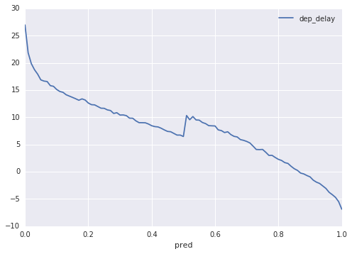
Figure 10-17. Where the model makes many of its errors
We could similarly analyze the performance of the model by each input variable (taxi-out distance, origin airport, etc.). For the sake of conciseness,16 let’s evaluate the model by just one variable, and to make it somewhat interesting, let’s pick a categorical variable—the carrier.
The query groups and aggregates by the categorical variable:
SELECT
  carrier, pred, AVG(dep_delay) as dep_delay
FROM
  flights2016.eval
WHERE (ontime > 0.5 and pred <= 0.5) or (ontime < 0.5 and pred > 0.5)
GROUP BY pred, carrier
The Pandas plot pulls out the corresponding groups and draws a separate line for each carrier:
df = df.sort_values(by='pred')
fig, ax = plt.subplots(figsize=(8,12))
for label, dfg in df.groupby('carrier'):
    dfg.plot(x='pred', y='dep_delay', ax=ax, label=label)
plt.legend();
Figure 10-18 shows the resulting plot.

Figure 10-18. How the model treats different carriers
Identifying Behavioral Change
Looking at Figure 10-18, it appears that the average departure delay for our false positives17 is lowest for flights operated by OO (SkyWest Airlines). Conversely, average departure delays are highest for our misses on flights operated by WN (Southwest Airlines). Observations like this would lead us to examine what has changed between 2015 and 2016 in the way these two carriers operate and ensure that we are capturing this difference when we retrain our model on new data. For example, Skywest might have changed its scheduling algorithm to add extra minutes to its nominal flight times, leading to flights that would have been late in 2015 arriving on time in 2016.
Let’s do a spot-check to see whether this is the case. Let’s find the most common flight flown by OO:
SELECT
  origin,
  dest,
  COUNT(*) as num_flights
FROM
  flights2016.eval
WHERE
  carrier = 'OO'
GROUP BY
  origin,
  dest
order by num_flights desc limit 10
Now, let’s look at the statistics of that flight (ORD-MKE) in 2015 and 2016:
SELECT
  APPROX_QUANTILES(TIMESTAMP_DIFF(CRS_ARR_TIME, CRS_DEP_TIME, SECOND), 5)
FROM
  flights2016.simevents
WHERE
  carrier = 'OO' and origin = 'ORD' and dest = 'MKE'
Indeed, the quantiles for scheduled flight times between Chicago (ORD) and Milwaukee (MKE) in 2016 are as follows:
2580, 2820, 2880, 2940, 3180
Here are the corresponding quantiles in 2015:
2400, 2760, 2880, 3060, 3300.
It’s worth unpacking this. The median scheduled time of a flight from Chicago to Milwaukee is the same. The median, of course, means that half the flights are scheduled to be shorter and the other half to be longer. The shorter flights in 2015 had a median scheduled time of 2,760 seconds; in 2016, this is 60 seconds longer. In other words, the airline has added more time to flights that were quite tight. On the other hand, the longer flights in 2015 had a median scheduled time of 3,060 minutes; in 2016, this was 120 minutes less. This sort of change in the underlying statistics of the system we are modeling illustrates why continuous machine learning training is so essential.
Summary
In this chapter, we completed the end-to-end process that we started in Chapter 1. We deployed the trained machine learning model as a microservice and embedded this microservice into a real-time streaming Cloud Dataflow pipeline. To do this, we had to convert Flight objects to JSON requests and take the JSON responses and create FlightPred objects for use in the pipeline. We also noticed that sending requests for flights one at a time could prove costly in terms of networking, money, and time. So, we batched up the requests to the machine learning service from within our Cloud Dataflow pipeline.
Our pipeline reads data from Cloud Pub/Sub, flattening the PCollection from each of the topics into a common PCollection that is processed by code that is identical to that used in training. Using the same code for serving as we used in training helps us mitigate training–serving skew. We also employed watermarks and triggers to gain a finer control on how to deal with late-arriving, out-of-order records.
We also explored other possible streaming sinks and how to choose between them. As a hypothetical, we implemented a Cloud Bigtable sink to work in situations for which high throughput and low latency are required. We designed an appropriate row-key to parallelize the writes while getting speedy reads.
Finally, we looked at how to evaluate model performance and recognize when a model is no longer valid because of behavioral changes by the key actors in the system we are modeling. We illustrated this by discovering a change in the flight scheduling of Skywest Airlines between 2015 and 2016. Behavioral changes like this are why machine learning is never done. Having now built an end-to-end system, we move on to continually improving it and constantly refreshing it with data.
Book Summary
In Chapter 1, we discussed the goals of data analysis, how to provide data-driven guidance using statistical and machine learning models, and the roles that will be involved with such work in the future. We also formulated our case study problem—of recommending whether a traveler should cancel a scheduled meeting based on the likelihood of the flight that they are on is delayed.
In Chapter 2, we automated the ingest of flight data from the BTS website. We began by reverse-engineering a web form, writing Python scripts to download the necessary data, and storing the data on Google Cloud Storage. Finally, we made the ingest process serverless by creating an App Engine application to carry out the ingest, and made it invokable from App Engine’s Cron service.
In Chapter 3, we discussed why it was important to bring end users’ insights into our data modeling efforts as early as possible. We achieved this by building a dashboard in Data Studio and populated this dashboard from Cloud SQL. We used the dashboard to explain a simple contingency table model that predicted on-time arrival likelihood by thresholding the departure delay of the flight.
In Chapter 4, we simulated the flight data as if it were arriving in real time, used the simulation to populate messages into Cloud Pub/Sub and then processed the streaming messages in Cloud Dataflow. In Cloud Dataflow, we computed aggregations and streamed the results into BigQuery. Because Cloud Dataflow follows the Beam programming model, the code for streaming and batch is the same, and this greatly simplified the training and operationalization of machine learning models in the rest of the book.
In Chapter 5, we carried out interactive data exploration by loading our dataset into Google BigQuery and plotting charts using Cloud Datalab. The model we used in this chapter was a nonparametric estimation of the 30th percentile of arrival delays. It was in this chapter that we also divided up our dataset into two parts—one part for training and the other for evaluation. We discussed why partitioning the dataset based on date was the right approach for this problem.
In Chapter 6, we created a Bayesian model on a Cloud Dataproc cluster. The Bayesian model itself involved quantization in Spark and on-time arrival percentage computation using Apache Pig. Cloud Dataproc allowed us to integrate BigQuery, Spark SQL, and Apache Pig into a Hadoop workflow. Because we stored our data on Google Cloud Storage (and not HDFS), our Cloud Dataproc cluster was job-specific and could be job-scoped, thus limiting our costs.
In Chapter 7, we built a logistic regression machine learning model using Apache Spark. The model had three input variables, all of which were continuous features. On adding categorical features, we found that the resulting explosion in the size of the dataset caused scalability issues. There were also significant hurdles to taking the logistic regression model and making it operational in terms of achieving low-latency predictions.
In Chapter 8, we built a Cloud Dataflow pipeline to compute time-aggregate features to use as inputs to a machine learning model. This involved the use of windows and side inputs, and grouping multiple parallel collections by key.
In Chapter 9, we used TensorFlow to create a wide-and-deep model with hand-crafted features, resulting in a high-performing model for predicting the on-time arrival probability. We scaled out the training of the TensorFlow model by using Cloud ML Engine, carried out hyperparameter tuning, and deployed the model so as to be able to carry out online predictions.
Finally, in this chapter, we pulled it all together by using the deployed model as a microservice, batching up calls to it and adding flight predictions as we receive and process flight data in real time. We also evaluated the model on completely independent data, learning that continuous training of our machine learning model is a necessity.
Throughout this book, as we worked our way through a data science problem end-to-end, from ingest to machine learning, the realization struck me that this is now a lot easier than it ever has been. I was able to do everything from simple thresholds to Bayesian techniques to deep-belief neural networks, with surprisingly little effort. At the same time, I was able to ingest data, refresh it, build dashboards, do stream processing, and operationalize the machine learning model with very little code. At the start of my career, 80% of the time to answer a data science question would be spent building the plumbing to get at the data. Making a machine learning model operational was something on the same scale as developing it in the first place. Google Cloud Platform, though, is designed to allow you to forget about infrastructure, and making a machine learning model operational is something you can fold into the model development phase itself. The practice of data science has become easier thanks to the advent of serverless data processing and machine learning systems that are integrated into powerful statistical and visualization software tools.
I can’t wait to see what you build next.
1 I am assuming that the number of users of our flight delay prediction service will be a factor of magnitude more than the number of flights. This is optimistic, of course, but it is good to design assuming that we will have a successful product.
2 The names of the attributes in the JSON (dep_delay, taxiout, etc.) are because we defined them in the serving_input_fn of our model’s export signature in Chapter 9. Specifically, we defined a placeholder for dep_delay as:
tf.placeholder(tf.float32, [None])
and a placeholder for origin as:
tf.placeholder(tf.string, [None])
This is why we are sending a floating-point value for dep_delay and a string value for origin.
3 Recall from Chapter 8 that I’m using Beam Java and not Beam Python because, as of this writing, Beam Python does not support streaming.
4 For the full code, go to https://github.com/GoogleCloudPlatform/data-science-on-gcp/blob/master/10_realtime/chapter10/src/main/java/com/google/cloud/training/flights/FlightsMLService.java.
5 For the full code, go to https://github.com/GoogleCloudPlatform/data-science-on-gcp/blob/master/10_realtime/chapter10/src/main/java/com/google/cloud/training/flights/AddRealtimePrediction.java.
6 You see multiple peaks in the chart because the pipeline sends requests to the machine learning service periodically, triggering on the end of a sliding time window.
7 The actual code for this is a bit more complex because we’d like to process wheelsoff, arrived, and canceled/diverted flights differently. So, the event type is made part of the key, and thus we create NUM_BATCHES*3 unique keys. For the full code, go to https://github.com/GoogleCloudPlatform/data-science-on-gcp/blob/master/10_realtime/chapter10/src/main/java/com/google/cloud/training/flights/InputOutput.java.
8 If we had a real-time feed, we’d of course collect data on delay instead of simply guessing.
9 See the jitter variable in https://github.com/GoogleCloudPlatform/data-science-on-gcp/blob/master/04_streaming/simulate/simulate.py.
10 The exception is for operations like an atomic increment, for which Cloud Bigtable expects the data to be an integer.
11 As of this writing, clusters and instances are one-to-one.
12 This location is in central Missouri. See https://www.census.gov/2010census/data/center-of-population.php.
13 Make sure you are using Standard SQL and not Legacy SQL.
15 In the evaluation Cloud Dataflow pipeline, we rounded this off to two digits.
16 I’m ready to finish writing this book!
17 Because our machine learning model is about predicting the probability of on-time arrival, false positives are those flights that arrived on time and for which the predicted probability was near 0.