
Chapter 8. Cloud APIs for Computer Vision: Up and Running in 15 Minutes
Due to repeated incidents of near meltdown at the nearby nuclear power plant, the library of the city of Springfield (we are not allowed to mention the state) decided that it was too risky to store all their valuable archives in physical form. After hearing that the library from their rival city of Shelbyville started digitizing their records, they wanted to get in on the game as well. After all, their collection of articles such as “Old man yells at cloud” and “Local man thinks wrestling is real” and the hundred-year-old iconic photographs of the Gorge and the statue of the city’s founder Jebediah Springfield are irreplaceable. In addition to making their archives resilient to catastrophes, they would make their archives easily searchable and retrievable. And, of course, the residents of Springfield now would be able to access all of this material from the comfort of their living room couches.
The first step in digitizing documents is, of course, scanning. That’s the easy part. Then starts the real challenge—processing and understanding all of this visual imagery. The team in Springfield had a few different options in front of them.
-
Perform manual data entry for every single page and every single photograph. Given that the city has more than 200 years of rich history, it would take a really long time, and would be error prone and expensive. It would be quite an ordeal to transcribe all of that material.
-
Hire a team of data scientists to build an image understanding system. That would be a much better approach, but there’s just one tiny hitch in the plan. For a library that runs on charitable donations, hiring a team of data scientists would quickly exhaust its budget. A single data scientist might not only be the highest-paid employee at the library, they might also be the highest-earning worker in the entire city of Springfield (barring the wealthy industrialist Montgomery Burns).
-
Get someone who knows enough coding to use the intelligence of ready-to-use vision APIs.
Logically they went with the quick and inexpensive third option. They had a stroke of luck, too. Martin Prince, an industrious fourth grader from Springfield Elementary who happened to know some coding, volunteered to build out the system for them. Although Martin did not know much deep learning (he’s just 10 years old, after all), he did know how to do some general coding, including making REST API calls using Python. And that was all he really needed to know. In fact, it took him just under 15 minutes to figure out how to make his first API call.
Martin’s modus operandi was simple: send a scanned image to the cloud API, get a prediction back, and store it in a database for future retrieval. And obviously, repeat this process for every single record the library owned. He just needed to select the correct tool for the job.
All the big names—Amazon, Google, IBM, Microsoft—provide a similar set of computer-vision APIs that label images, detect and recognize faces and celebrities, identify similar images, read text, and sometimes even discern handwriting. Some of them even provide the ability to train our own classifier without having to write a single line of code. Sounds really convenient!
In the background, these companies are constantly working to improve the state of the art in computer vision. They have spent millions in acquiring and labeling datasets with a granular taxonomy much beyond the ImageNet dataset. We might as well make good use of their researchers’ blood, sweat, and tears (and electricity bills).
The ease of use, speed of onboarding and development, the variety of functionality, richness of tags, and competitive pricing make cloud-based APIs difficult to ignore. And all of this without the need to hire an expensive data science team. Chapters Chapter 5 and Chapter 6 optimized for accuracy and performance, respectively; this chapter essentially optimizes for human resources.
In this chapter, we explore several cloud-based visual recognition APIs. We compare them all both quantitatively as well as qualitatively. This should hopefully make it easier to choose the one that best suits your target application. And if they still don’t match your needs, we’ll investigate how to train a custom classifier with just a few clicks.
(In the interest of full disclosure, some of the authors of this book were previously employed at Microsoft, whose offerings are discussed here. We have attempted not to let that bias our results by building reproducible experiments and justifying our methodology.)
The Landscape of Visual Recognition APIs
Let’s explore some of the different visual recognition APIs out there.
Clarifai
Clarifai (Figure 8-1) was the winner of the 2013 ILSVRC classification task. Started by Matthew Zeiler, a graduate student from New York University, this was one of the first visual recognition API companies out there.
Note
Fun fact: While investigating a classifier to detect NSFW (Not Safe For Work) images, it became important to understand and debug what was being learned by the CNN in order to reduce false positives. This led Clarifai to invent a visualization technique to expose which images stimulate feature maps at any layer in the CNN. As they say, necessity is the mother of invention.
What’s unique about this API?
It offers multilingual tagging in more than 23 languages, visual similarity search among previously uploaded photographs, face-based multicultural appearance classifier, photograph aesthetic scorer, focus scorer, and embedding vector generation to help us build our own reverse-image search. It also offers recognition in specialized domains including clothing and fashion, travel and hospitality, and weddings. Through its public API, the image tagger supports 11,000 concepts.

Figure 8-1. Sample of Clarifai’s results
Microsoft Cognitive Services
With the creation of ResNet-152 in 2015, Microsoft was able to win seven tasks at the ILSVRC, the COCO Image Captioning Challenge as well as the Emotion Recognition in the Wild challenge, ranging from classification and detection (localization) to image descriptions. And most of this research was translated to cloud APIs. Originally starting out as Project Oxford from Microsoft Research in 2015, it was eventually renamed Cognitive Services in 2016. It’s a comprehensive set of more than 50 APIs ranging from vision, natural language processing, speech, search, knowledge graph linkage, and more. Historically, many of the same libraries were being run at divisions at Xbox and Bing, but they are now being exposed to developers externally. Some viral applications showcasing creative ways developers use these APIs include how-old.net (How Old Do I Look?), Mimicker Alarm (which requires making a particular facial expression in order to defuse the morning alarm), and CaptionBot.ai.
What’s unique about this API?
As illustrated in Figure 8-2, the API offers image captioning, handwriting understanding, and headwear recognition. Due to many enterprise customers, Cognitive Services does not use customer image data for improving its services.

Figure 8-2. Sample of Microsoft Cognitive Services results
Google Cloud Vision
Google provided the winning entry at the 2014 ILSVRC with the help of the 22-layer GoogLeNet, which eventually paved the way for the now-staple Inception architectures. Supplementing the Inception models, in December 2015, Google released a suite of Vision APIs. In the world of deep learning, having large amounts of data is definitely an advantage to improve one’s classifier, and Google has a lot of consumer data. For example, with learnings from Google Street View, you should expect relatively good performance in real-world text extraction tasks, like on billboards.
What’s unique about this API?
For human faces, it provides the most detailed facial key points (Figure 8-3) including roll, tilt, and pan to accurately localize the facial features. The APIs also return similar images on the web to the given input. A simple way to try out the performance of Google’s system without writing code is by uploading photographs to Google Photos and searching through the tags.

Figure 8-3. Sample of Google Cloud Vision’s results
Amazon Rekognition
No, that title is not a typo. Amazon Rekognition API (Figure 8-4) is largely based on Orbeus, a Sunnyvale, California-based startup that was acquired by Amazon in late 2015. Founded in 2012, its chief scientist also had winning entries in the ILSVRC 2014 detection challenge. The same APIs were used to power PhotoTime, a famous photo organization app. The API’s services are available as part of the AWS offerings. Considering most companies already offer photo analysis APIs, Amazon is doubling down on video recognition offerings to offer differentiation.
What’s unique about this API?
License plate recognition, video recognition APIs, and better end-to-end integration examples of Rekognition APIs with AWS offerings like Kinesis Video Streams, Lambda, and others. Also, Amazon’s API is the only one that can determine whether the subject’s eyes are open or closed.

Figure 8-4. Sample of Amazon Rekognition’s results
IBM Watson Visual Recognition
Under the Watson brand, IBM’s Visual Recognition offering started in early 2015. After purchasing AlchemyAPI, a Denver-based startup, AlchemyVision has been used for powering the Visual Recognition APIs (Figure 8-5). Like others, IBM also offers custom classifier training. Surprisingly, Watson does not offer optical character recognition yet.

Figure 8-5. Sample of IBM Watson’s Visual Recognition results
Algorithmia
Algorithmia is a marketplace for hosting algorithms as APIs on the cloud. Founded in 2013, this Seattle-based startup has both its own in-house algorithms as well as those created by others (in which case creators earn revenue based on the number of calls). In our experience, this API did tend to have the slowest response time.
What’s unique about this API?
Colorization service for black and white photos (Figure 8-6), image stylization, image similarity, and the ability to run these services on-premises, or on any cloud provider.

Figure 8-6. Sample of Algorithmia’s style transfer results
With so many offerings, it can be overwhelming to choose a service. There are many reasons why we might choose one over another. Obviously, the biggest factors for most developers would be accuracy and price. Accuracy is the big promise that the deep learning revolution brings, and many applications require it on a consistent basis. Price of the service might be an additional factor to consider. We might also choose a service provider because our company already has a billing account with it, and it would take additional effort to integrate a different service provider. Speed of the API response might be another factor, especially if the user is waiting on the other end for a response. Because many of these API calls can be abstracted, it’s easy to switch between different providers.
Comparing Visual Recognition APIs
To aid our decision making, let’s compare these APIs head to head. In this section, we examine service offerings, cost, and accuracy of each.
Service Offerings
Table 8-1 lists what services are being offered by each cloud provider.
| Algorithmia | Amazon Rekognition | Clarifai | Microsoft Cognitive Services | Google Cloud Vision | IBM Watson Visual Recognition | |
|---|---|---|---|---|---|---|
| Image classification |
✔ |
✔ |
✔ |
✔ |
✔ |
✔ |
| Image detection |
✔ |
✔ |
|
✔ |
✔ |
|
| OCR |
✔ |
✔ |
|
✔ |
✔ |
|
| Face recognition |
✔ |
✔ |
|
✔ |
|
|
|
Emotion recognition |
✔ |
|
✔ |
✔ |
✔ |
|
| Logo recognition |
|
|
✔ |
✔ |
✔ |
|
| Landmark recognition |
|
|
✔ |
✔ |
✔ |
✔ |
|
Celebrity recognition |
✔ |
✔ |
✔ |
✔ |
✔ |
✔ |
| Multilingual tagging |
|
|
✔ |
|
|
|
| Image description |
|
|
|
✔ |
|
|
| Handwriting |
|
|
|
✔ |
✔ |
|
| Thumbnail generation |
✔ |
|
|
✔ |
✔ |
|
| Content moderation |
✔ |
✔ |
✔ |
✔ |
✔ |
|
| Custom classification training |
|
|
✔ |
✔ |
✔ |
✔ |
| Custom detector training |
|
✔ |
✔ |
|||
| Mobile custom models |
✔ |
✔ |
✔ |
|||
| Free tier | 5,000 requests per month | 5,000 requests per month | 5,000 requests per month | 5,000 requests per month | 1,000 requests per month | 7,500 |
That’s a mouthful of services already up and running, ready to be used in our application. Because numbers and hard data help make decisions easier, it’s time to analyze these services on two factors: cost and accuracy.
Cost
Money doesn’t grow on trees (yet), so it’s important to analyze the economics of using off-the-shelf APIs. Taking a heavy-duty example of querying these APIs at about 1 query per second (QPS) service for one full month (roughly 2.6 million requests per month), Figure 8-7 presents a comparison of the different providers sorted by estimated costs (as of August 2019).

Figure 8-7. A cost comparison of different cloud-based vision APIs
Although for most developers, this is an extreme scenario, this would be a pretty realistic load for large corporations. We will eventually compare these prices against running our own service in the cloud to make sure we get the most bang for the buck fitting our scenario.
That said, many developers might find negligible charges, considering that all of the cloud providers we look at here have a free tier of 5,000 calls per month (except Google Vision, which gives only 1,000 calls per month for free), and then roughly $1 per 1,000 calls.
Accuracy
In a world ruled by marketing departments who claim their organizations to be the market leaders, how do we judge who is actually the best? What we need are common metrics to compare these service providers on some external datasets.
To showcase building a reproducible benchmark, we assess the text extraction quality using the COCO-Text dataset, which is a subset of the MS COCO dataset. This 63,686-image set contains text in daily life settings, like on a banner, street sign, number on a bus, price tag in a grocery store, designer shirt, and more. This real-world imagery makes it a relatively tough set to test against. We use the Word Error Rate (WER) as our benchmarking metric. To keep things simple, we ignore the position of the word and focus only on whether a word is present (i.e., bag of words). To be a match, the entire word must be correct.
In the COCO-Text validation dataset, we pick all images with one or more instances of legible text (full-text sequences without interruptions) and compare text instances of more than one-character length. We then send these images to various cloud vision APIs. Figure 8-8 presents the results.

Figure 8-8. WER for different text extraction APIs as of August 2019
Considering how difficult the dataset is, these results are remarkable. Most state-of-the-art text extraction tools from earlier in the decade would not cross the 10% mark. This shows the power of deep learning. On a subset of manually tested images, we also noticed a year-on-year improvement in the performance of some of these APIs, which is another benefit enjoyed by cloud-based APIs.
As always, all of the code that we used for our experiment is hosted on GitHub (see http://PracticalDeepLearning.ai.
The results of our analysis depend significantly on the dataset we choose as well as our metrics. Depending on our dataset (which is in turn influenced by our use case) as well as our minimum quality metrics, our results can vary. Additionally, service providers are constantly improving their services in the background. As a consequence, these results are not set in stone and improve over time. These results can be replicated on any dataset with the scripts on GitHub.
Bias
In Chapter 1, we explored how bias can creep into datasets and how it can have real-life consequences for people. The APIs we explore in this chapter are no exception. Joy Buolamwini, a researcher at the MIT Media Lab, discovered that among Microsoft, IBM, and Megvii (also known as Face++), none were able to detect her face and gender accurately. Wondering if she had unique facial features that made her undetectable to these APIs, she (working along with Timnit Gebru) compiled faces of members of legislative branches from six countries with a high representation of women, building the Pilot Parliaments Benchmark (PPB; see Figure 8-9). She chose members from three African countries and three European countries to test for how the APIs performed on different skin tones. If you haven’t been living under a rock, you can already see where this is going.
She observed that the APIs performed fairly well overall at accuracies between 85% and 95%. It was only when she started slicing the data across the different categories that she observed there was a massive amount of difference in the accuracies for each. She first observed that there was a significant difference between detection accuracies of men and women. She also observed that breaking down by skin tone, the difference in the detection accuracy was even larger. Then, finally, taking both gender and skin tone into consideration, the differences grew painfully starker between the worse detected group (darker females) and the best detected group (lighter males). For example, in the case of IBM, the detection accuracy of African women was a mere 65.3%, whereas the same API gave a 99.7% accuracy for European men. A whopping 34.4% difference! Considering many of these APIs are used by law enforcement, the consequences of bias seeping in might have life or death consequences.

Figure 8-9. Averaged faces among different gender and skin tone, from Pilot Parliaments Benchmark (PPB)
Following are a few insights we learned from this study:
-
The algorithm is only as good as the data on which it’s trained. And this shows the need for diversity in the training dataset.
-
Often the aggregate numbers don’t always reveal the true picture. The bias in the dataset is apparent only when slicing it across different subgroups.
-
The bias does not belong to any specific company; rather, it’s an industry-wide phenomenon.
-
These numbers are not set in stone and reflect only the time at which the experiment was performed. As evident from the drastic change in numbers between 2017 (Figure 8-10) and a subsequent study in 2018 (Figure 8-11), these companies are taking bias removal from their datasets quite seriously.
-
Researchers putting commercial companies to the test with public benchmarks results in industry-wide improvements (even if for the fear of bad PR, then so be it).

Figure 8-10. Face detection comparison across APIs, tested in April and May 2017 on the PPB

Figure 8-11. Face detection comparison across APIs in August 2018 on the PPB, conducted by Inioluwa Deborah Raji et al.
How about bias in image-tagging APIs? Facebook AI Research pondered over the question “Does Object Recognition Work for Everyone?” in a paper by the same title (Terrance DeVries et al.). The group tested multiple cloud APIs in February 2019 on Dollar Street, a diverse collection of images of household items from 264 different homes across 50 countries (Figure 8-12).

Figure 8-12. Image-tagging API performance on geographically diverse images from the Dollar Street dataset
Here are some of the key learnings from this test:
-
Accuracy of object classification APIs was significantly lower in images from regions with lower income levels, as illustrated in Figure 8-13.
-
Datasets such as ImageNet, COCO, and OpenImages severely undersample images from Africa, India, China, and Southeast Asia, hence leading to lower performance on images from the non-Western world.
-
Most of the datasets were collected starting with keyword searches in English, omitting images that mentioned the same object with phrases in other languages.

Figure 8-13. Average accuracy (and standard deviation) of six cloud APIs versus income of the household where the images were collected
In summary, depending on the scenario for which we want to use these cloud APIs, we should build our own benchmarks and test them periodically to evaluate whether these APIs are appropriate for the use case.
Getting Up and Running with Cloud APIs
Calling these cloud services requires minimal code. At a high level, get an API key, load the image, specify the intent, make a POST request with the proper encoding (e.g., base64 for the image), and receive the results. Most of the cloud providers offer software development kits (SDKs) and sample code showcasing how to call their services. They additionally provide pip-installable Python packages to further simplify calling them. If you’re using Amazon Rekognition, we highly recommend using its pip package.
Let’s reuse our thrilling image to test-run these services.
First, let’s try it on Microsoft Cognitive Services. Get an API key and replace it in the following code (the first 5,000 calls are free—more than enough for our experiments):
cognitive_services_tagimage('DogAndBaby.jpg')

Results:
{"description":{"tags":["person","indoor","sitting","food","table","little","small","dog","child","looking","eating","baby","young","front","feeding","holding","playing","plate","boy","girl","cake","bowl","woman","kitchen","standing","birthday","man","pizza"],"captions":[{"text":"a little girl sitting at a table with a dog","confidence":0.84265453815486435}]},"requestId":"1a32c16f-fda2-4adf-99b3-9c4bf9e11a60","metadata":{"height":427,"width":640,"format":"Jpeg"}}
“A little girl sitting at a table with a dog”—pretty close! There are other options to generate more detailed results, including a probability along with each tag.
Tip
Although the ImageNet dataset is primarily tagged with nouns, many of these services go beyond and return verbs like “eating,” “sitting,” “jumping.” Additionally, they might contain adjectives like “red.” Chances are, these might not be appropriate for our application. We might want to filter out these adjectives and verbs. One option is to check their linguistic type against Princeton’s WordNet. This is available in Python with the Natural Language Processing Toolkit (NLTK). Additionally, we might want to filter out words like “indoor” and “outdoor” (often shown by Clarifai and Cognitive Services).
Now, let’s test the same image using Google Vision APIs. Get an API key from their website and use it in the following code (and rejoice, because the first 1,000 calls are free):
google_cloud_tagimage('DogAndBaby.jpg')

Results:
{"responses":[{"labelAnnotations":[{"mid":"/m/0bt9lr","description":"dog","score":0.951077,"topicality":0.951077},{"mid":"/m/06z04","description":"skin","score":0.9230451,"topicality":0.9230451},{"mid":"/m/01z5f","description":"dog like mammal","score":0.88359463,"topicality":0.88359463},{"mid":"/m/01f5gx","description":"eating","score":0.7258142,"topicality":0.7258142}#otherobjects]}]}
Wasn’t that a little too easy? These APIs help us get to state-of-the-art results without needing a Ph.D.—in just 15 minutes!
Tip
Even though these services return tags and image captions with probabilities, it’s up to the developer to determine a threshold. Usually, 60% and 40% are good thresholds for image tags and image captions, respectively.
It’s also important to communicate the probability to the end-user from a UX standpoint. For example, if the result confidence is >80%, we might say prefix the tags with “This image contains....” For <80%, we might want to change that prefix to “This image may contain…” to reflect the lower confidence in the result.
Training Our Own Custom Classifier
Chances are these services were not quite sufficient to meet the requirements of our use case. Suppose that the photograph we sent to one of these services responded with the tag “dog.” We might be more interested in identifying the breed of the dog. Of course, we can follow Chapter 3 to train our own classifier in Keras. But wouldn’t it be more awesome if we didn’t need to write a single line of code? Help is on the way.
A few of these cloud providers give us the ability to train our own custom classifier by merely using a drag-and-drop interface. The pretty user interfaces provide no indication that under the hood they are using transfer learning. As a result, Cognitive Services Custom Vision, Google AutoML, Clarifai, and IBM Watson all provide us the option for custom training. Additionally, some of them even allow building custom detectors, which can identify the location of objects with a bounding box. The key process in all of them being the following:
-
Upload images
-
Label them
-
Train a model
-
Evaluate the model
-
Publish the model as a REST API
-
Bonus: Download a mobile-friendly model for inference on smartphones and edge devices
Let’s see a step-by-step example of Microsoft’s Custom Vision.
-
Create a project (Figure 8-14): Choose a domain that best describes our use case. For most purposes, “General” would be optimal. For more specialized scenarios, we might want to choose a relevant domain.

Figure 8-14. Creating a new project in Custom Vision
As an example, if we have an ecommerce website with photos of products against a pure white background, we might want to select the “Retail” domain. If we intend to run this model on a mobile phone eventually, we should choose the “Compact” version of the model, instead; it is smaller in size with only a slight loss in accuracy.
-
Upload (Figure 8-15): For each category, upload images and tag them. It’s important to upload at least 30 photographs per category. For our test, we uploaded more than 30 images of Maltese dogs and tagged them appropriately.

Figure 8-15. Uploading images on CustomVision.ai
-
Train (Figure 8-16): Click the Train button, and then in about three minutes, we have a spanking new classifier ready.

Figure 8-16. The Train button in the upper-right corner of the CustomVision.ai page
-
Analyze the model’s performance: Check the precision and recall of the model. By default, the system sets the threshold at 90% confidence and gives the precision and recall metrics at that value. For higher precision, increase the confidence threshold. This would come at the expense of reduced recall. Figure 8-17 shows example output.
-
Ready to go: We now have a production-ready API endpoint that we can call from any application.
To highlight the effect of the amount of data on model quality, let’s train a dog breed classifier. We can use the Stanford Dogs dataset, a collection of more than 100 dog categories. For simplicity, we randomly chose 10 breeds, which have more than 200 images available. With 10 classes, a random classifier would have one-tenth, or 10%, the chance of correctly identifying an image. We should easily be able to beat this number. Table 8-2 shows the effect of training on datasets with different volumes.
| 30 training images/class | 200 training images/class | |
|---|---|---|
| Precision | 91.2% | 93.5% |
| Recall | 85.3% | 89.6% |

Figure 8-17. Relative precision and recall for our sample training set with 200 images per class
Because we haven’t uploaded a test set, the performance figures reported here are on the full dataset using the common k-fold cross-validation technique. This means the data was randomly divided into k parts, then (k – 1) parts were used for training, and the remaining part was used for testing. This was performed a few times, each time with a randomized subset of images, and the averaged results are reported here.
It is incredible that even with 30 images per class, the classifier’s precision is greater than 90%, as depicted in Figure 8-18. And, surprisingly, this took slightly less than 30 seconds to train.
Not only this, we can dig down and investigate the performance on each class. Classes with high precision might visibly be more distinct, whereas those with low precision might look similar to another class.

Figure 8-18. Some of the possible tags returned by the API
This short and convenient approach is not without its downsides, as you will see in the following section. In that section, we also discuss mitigation strategies to help take advantage of this rather useful tool.
Top Reasons Why Our Classifier Does Not Work Satisfactorily
There are a number of reasons why a classifier would not perform well. The following are some of them:
- Not enough data
-
If we find that the accuracy is not quite sufficient for our needs, we might need to train the system with more data. Of course, 30 images per class just gets us started. But for a production-quality application, more images are better. 200 images per class are usually recommended.
- Nonrepresentative training data
-
Often, the images on the internet are far too clean, set up in studio lighting with clean backgrounds, and close to the center of the frame. Images that our application might see on a daily basis might not be represented quite so well. It’s really important to train our classifier with real-world images for the best performance.
- Unrelated domain
- Under the hood, Custom Vision is running transfer learning. This makes it really important to choose the correct domain when creating the project. As an example, if we are trying to classify X-ray images, transfer learning from an ImageNet-based model might not yield as accurate a result. For cases like that, training our own classifier manually in Keras would work best, as demonstrated in Chapter 3 (though this will probably take more than three minutes).
- Using it for regression
-
In machine learning, there are two common categories of problems: classification and regression. Classification is predicting one or more classes for input. Regression, on the other hand, is predicting a numerical value given an input; for example, predicting house prices. Custom Vision is primarily a classification system. Using it to count objects by tagging the number of objects is the wrong approach, and will lead to unsatisfactory results.
Counting objects is a type of regression problem. We can do it by localizing each instance of the object in an image (aka object detection) and counting their occurrences. Another example of a regression problem is predicting the age of a person based on their profile photo. We tackle both problems in later chapters.
- Classes are too similar
-
If our classes look too similar and rely heavily on smaller-level details for distinction, the model might not perform as well. For example, a five-dollar note and a 20-dollar note have very similar high-level features. It’s at the lower-level details that show they are really distinct. As another example, it might be easy to distinguish between a Chihuahua and a Siberian Husky, but it’s more difficult to distinguish between an Alaskan Malamute and a Siberian Husky. A fully retrained CNN, as demonstrated in Chapter 3, should perform better than this Custom Vision-based system.
Tip
A great feature of Custom Vision is that if the model is unsure of any image that it encounters via its API endpoint, the web UI will show those images for a manual review. We can review and manually tag new images on a periodic basis and continuously improve the quality of the model. These images tend to improve the classifier the most for two reasons: first, they represent real-world usage. Second, and more importantly, they have more impact on the model in comparison to images that the model can already easily classify. This is known as semisupervised learning.
In this section, we discussed a few different ways in which we can improve our model’s accuracy. In the real world, that is not the end-all-be-all of a user’s experience. How quickly we are able to respond to a request also matters a lot. In the following section, we cover a couple of different ways we can improve performance without sacrificing quality.
Comparing Custom Classification APIs
As you might have noticed throughout the book, we are pretty dogmatic about being data driven. If we are going to spend good money on a service, we better get the best bang for our buck. Time to put the hype to the test.
For a good number of classification problems, these custom cloud-based classifiers perform pretty well. To truly test their limits, we need something more challenging. We need to unleash the toughest doggone dataset, train this animal, and fetch some insightful results—using the Stanford Dogs dataset.
Using the entire dataset might make it too easy for these classifiers (after all, ImageNet already has so many dog breeds), so we took it up a notch. Instead, we trained our own Keras classifier on the entire dataset and built a mini-dataset out of the top 34 worst-performing classes (each containing at least 140 images). The reason these classes performed poorly was because they often became confused with other similar-looking dog breeds. To perform better, they require a fine-grained understanding of the features. We divide the images into 100 randomly chosen images per class in the training dataset and 40 randomly chosen images per class in the test dataset. To avoid any class imbalances, which can have an impact on predictions, we chose the same number of train and test images for each class.
Lastly, we selected a minimum confidence threshold of 0.5 as it appeared to strike a good balance between precision and recall across all services. At a high confidence threshold such as 0.99, a classifier might be very accurate, but there might be only a handful of images with predictions; in other words, really low recall. On the other hand, a really low threshold of 0.01 would result in predictions for nearly all images. However, we should not rely on many of these results. After all, the classifier is not confident.
Instead of reporting the precision and recall, we report the F1 score (also known as F-measure), which is a hybrid score that combines both of those values:
Additionally, we report the time it took to train, as shown in Figure 8-19. Beyond just the cloud, we also trained using Apple’s Create ML tool on a MacBook Pro with and without data augmentations (rotate, crop, and flip).
Google and Microsoft provide the ability to customize the duration of training. Google Auto ML allows us to customize between 1 and 24 hours. Microsoft provides a free “Fast Training” option and a paid “Advanced Training” option (similar to Google’s offering) with which we can select the duration to be anywhere between 1 and 24 hours.

Figure 8-19. A chart showing the F1 score for custom classifier services, as of August 2019 (higher is better)
Following are some interesting takeaways from this experiment:
-
Clarifai and Microsoft offered near-instant training for the 3,400 training images.
-
Compared to “Fast Training,” Microsoft’s “Advanced Training” performed slightly better (roughly a 1-point increase) for the extra one hour of training. Because “Fast Training” took less than 15 seconds to train, we can infer that its base featurizer was already good at extracting fine-grained features.
-
Surprisingly, Apple’s Create ML actually performed worse after adding in the augmentations, despite taking more than two extra hours to train, most of which was spent creating the augmentations. This was done on a top-of-the-line MacBook Pro and showed 100% GPU utilization in Activity Monitor.
Additionally, to test the featurizer’s strength, we varied the amount of training data supplied to the service (Figure 8-20). Because Microsoft took less than 15 seconds to train, it was easy (and cheap!) for us to perform the experiment there. We varied between 30 and 100 images per class for training while keeping the same 40 images per class for testing.

Figure 8-20. Effect of varying size of training data per class on test F1 score (higher is better)
Even though Microsoft recommends using at least 50 images per class, going under that limit did not affect performance significantly. The fact that the F1 score did not vary as much as one would expect shows the value of transfer learning (enabling less data to build classifiers) and having a good featurizer capable of fine-grained classification.
It bears repeating that this experiment was intentionally made difficult to stress-test these classifiers. On average, they would have performed much better on the entire Stanford Dogs dataset.
Performance Tuning for Cloud APIs
A photograph taken by a modern cell phone can have a resolution as high as 4000 x 3000 pixels and be upward of 4 MB in size. Depending on the network quality, it can take a few seconds to upload such an image to the service. With each additional second, it can become more and more frustrating for our users. Could we make this faster?
There are two ways to reduce the size of the image:
- Resizing
-
Most CNNs take an input image with a size of 224 x 224 or 448 x 448 pixels. Much of a cell phone photo’s resolution would be unnecessary for a CNN. It would make sense to downsize the image prior to sending it over the network, instead of sending a large image over the network and then downsizing it on the server.
- Compression
-
Most image libraries perform lossy compression while saving a file. Even a little bit of compression can go a long way in reducing the size of the image while minimally affecting the quality of the image itself. Compression does introduce noise, but CNNs are usually robust enough to deal with some of it.
Effect of Resizing on Image Labeling APIs
We performed an experiment in which we took more than a hundred diverse unmodified images taken from an iPhone at the default resolution (4032 x 3024) and sent them to the Google Cloud Vision API to get labels for each of those images. We then downsized each of the original images in 5% increments (5%, 10%, 15%…95%) and collected the API results for those smaller images, too. We then calculated the agreement rate for each image using the following formula:
Figure 8-21 shows the results of this experiment. In the figure, the solid line shows the reduction in file size, and the dotted line represents the agreement rate. Our main conclusion from the experiment was that a 60% reduction in resolution led to a 95% reduction in file size, with little change in accuracy compared to the original images.
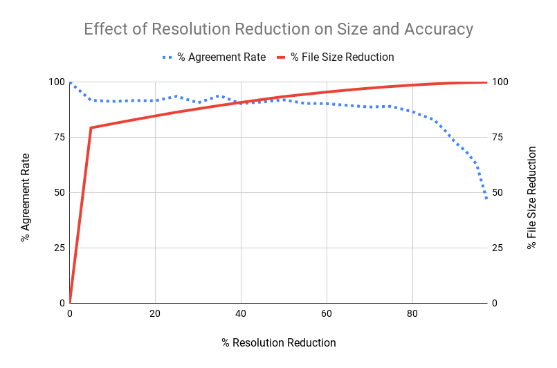
Figure 8-21. Effect of resizing an image on agreement rate and file size reduction relative to the original image
Effect of Compression on Image Labeling APIs
We repeated the same experiment, but instead of changing the resolution, we changed the compression factor for each image incrementally. In Figure 8-22, the solid line shows the reduction in file size and the dotted line represents the agreement rate. The main takeaway here is that a 60% compression score (or 40% quality) leads to an 85% reduction in file size, with little change in accuracy compared to the original image.

Figure 8-22. Effect of compressing an image on agreement rate and file size reduction relative to the original image
Effect of Compression on OCR APIs
We took a document containing 300-plus words at the default resolution of an iPhone (4032 x 3024), and sent it to the Microsoft Cognitive Services API to test text recognition. We then compressed it at 5% increments and then sent each image and compressed it. We sent these images to the same API and compared their results against the baseline to calculate the percentage WER. We observed that even setting the compression factor to 95% (i.e., 5% quality of the original image) had no effect on the quality of results.
Effect of Resizing on OCR APIs
We repeated the previous experiment, but this time by resizing each image instead of compressing. After a certain point, the WER jumped from none to almost 100%, with nearly all words being misclassified. Retesting this with another document having each word at a different font size showed that all words under a particular font size were getting misclassified. To effectively recognize text, OCR engines need the text to be bigger than a minimum height (a good rule of thumb is larger than 20 pixels). Hence the higher the resolution, the higher the accuracy.
What have we learned?
-
For text recognition, compress images heavily, but do not resize.
-
For image labeling, a combination of moderate resizing (say, 50%) and moderate compression (say, 30%) should lead to heavy file size reductions (and quicker API calls) without any difference in quality of API results.
-
Depending on your application, you might be working with already resized and compressed images. Every processing step can introduce a slight difference in the results of these APIs, so aim to minimize them.
Tip
After receiving an image, cloud APIs internally resize it to fit their own implementation. For us, this means two levels of resizing: we first resize an image to reduce the size, then send it to the cloud API, which further resizes the image. Downsizing images introduces distortion, which is more evident at lower resolutions. We can minimize the effect of distortion by resizing from a higher resolution, which is bigger by a few multiples. For example, resizing 3024x3024 (original) → 302x302 (being sent to cloud) → 224x224 (internally resized by APIs) would introduce much more distortion in the final image compared to 3024x3024 → 896x896 → 224x224. Hence, it’s best to find a happy intermediate size before sending the images. Additionally, specifying advanced interpolation options like BICUBIC and LANCZOS will lead to more accurate representation of the original image in the smaller version.
Case Studies
Some people say that the best things in life don’t come easy. We believe this chapter proves otherwise. In the following section, we take a look at how some tech industry titans use cloud APIs for AI to drive some very compelling scenarios.
The New York Times
It might seem like the scenario painted at the beginning of the chapter was taken out of a cartoon, but it was, in fact, pretty close to the case of the New York Times (NYT). With more than 160 years of illustrious history, NYT has a treasure trove of photographs in its archives. It stored many of these artifacts in the basement of its building three stories below the ground level, aptly called the “morgue.” The value of this collection is priceless. In 2015, due to a plumbing leak, parts of the basement were damaged including some of these archived records. Thankfully the damage was minimal. However, this prompted NYT to consider digitally archiving them to protect against another catastrophe.
The photographs were scanned and stored in high quality. However, the photographs themselves did not have any identifying information. What many of them did have were handwritten or printed notes on the backside giving context for the photographs. NYT used the Google Vision API to scan this text and tag the respective images with that information. Additionally, this pipeline provided opportunities to extract more metadata from the photographs, including landmark recognition, celebrity recognition, and so on. These newly added tags powered its search feature so that anyone within the company and outside could explore the gallery and search using keywords, dates, and so on without having to visit the morgue, three stories down.
Uber
Uber uses Microsoft Cognitive Services to identify each of its seven million-plus drivers in a couple of milliseconds. Imagine the sheer scale at which Uber must operate its new feature called “Real-Time ID Check.” This feature verifies that the current driver is indeed the registered driver by prompting them to take a selfie either randomly or every time they are assigned to a new rider. This selfie is compared to the driver’s photo on file, and only if the face models are a match is the driver allowed to continue. This security feature is helpful for building accountability by ensuring the security of the passengers and by ensuring that the driver’s account is not compromised. This safety feature is able to detect changes in the selfie, including a hat, beard, sunglasses, and more, and then prompts the driver to take a selfie without the hat or sunglasses.

Figure 8-23. The Uber Drivers app prompts the driver to take a selfie to verify the identity of the driver (image source)
Giphy
Back in 1976, when Dr. Richard Dawkins coined the term “meme,” little did he know it would take on a life of its own four decades later. Instead of giving a simple textual reply, we live in a generation where most chat applications suggest an appropriate animated GIF matching the context. Several applications provide a search specific to memes and GIFs, such as Tenor, Facebook messenger, Swype, and Swiftkey. Most of them search through Giphy (Figure 8-24), the world’s largest search engine for animated memes commonly in the GIF format.

Figure 8-24. Giphy extracts text from animations as metadata for searching
GIFs often have text overlaid (like the dialogue being spoken) and sometimes we want to look for a GIF with a particular dialogue straight from a movie or TV show. For example, the image in Figure 8-24 from the 2010 Futurama episode in which the “eyePhone” (sic) was released is often used to express excitement toward a product or an idea. Having an understanding of the contents makes the GIFs more searchable. To make this happen, Giphy uses Google’s Vision API to extract the recognize text and objects—aiding the search for the perfect GIF.
It’s obvious that tagging GIFs is a difficult task because a person must sift through millions of these animations and manually annotate them frame by frame. In 2017, Giphy figured out two solutions to automate this process. The first approach was to detect text from within the image. The second approach was to generate tags based on the objects in the image to supplement the metadata for their search engine. This metadata is stored and searched using ElasticSearch to make a scalable search engine.
For text detection, the company used the OCR services from the Google Vision API on the first frame from the GIFs to confirm whether the GIF actually contained text. If the API replied in the affirmative, Giphy would send the next frames, receive their OCR-detected texts, and figure out the differences in the text; for instance, whether the text was static (remaining the same throughout the duration of the gif) or dynamic (different text in different frames). For generating the class labels corresponding to objects in the image, engineers had two options: label detection or web entities, both of which are available on Google Vision API. Label detection, as the name suggests, provides the actual class name of the object. Web entities provides an entity ID (which can be referenceable in the Google Knowledge Graph), which is the unique web URL for identical and similar images seen elsewhere on the net. Using these additional annotations gave the new system an increase in the click-through-rate (CTR) by 32%. Medium-to-long-tail searches (i.e., not-so-frequent searches) benefitted the most, becoming richer with relevant content as the extracted metadata surfaced previously unannotated GIFs that would have otherwise been hidden. Additionally, this metadata and click-through behavior of users provides data to make a similarity and deduplication feature.
OmniEarth
OmniEarth is a Virginia-based company that specializes in collecting, analyzing, and combining satellite and aerial imagery with other datasets to track water usage across the country, scalably, and at high speeds. The company is able to scan the entire United States at a total of 144 million parcels of land within hours. Internally, it uses the IBM Watson Visual Recognition API to classify images of land parcels for valuable information like how green it is. Combining this classification with other data points such as temperature and rainfall, OmniEarth can predict how much water was used to irrigate the field.
For house properties, it infers data points from the image such as the presence of pools, trees, or irrigable landscaping to predict the amount of water usage. The company even predicted where water is being wasted due to malpractices like overwatering or leaks. OmniEarth helped the state of California understand water consumption by analyzing more than 150,000 parcels of land, and then devised an effective strategy to curb water waste.
Photobucket
Photobucket is a popular online image- and video-hosting community where more than two million images are uploaded every day. Using Clarifai’s NSFW models, Photobucket automatically flags unwanted or offensive user-generated content and sends it for further review to its human moderation team. Previously, the company’s human moderation team was able to monitor only about 1% of the incoming content. About 70% of the flagged images turned out to be unacceptable content. Compared to previous manual efforts, Photobucket identified 700 times more unwanted content, thus cleaning the website and creating a better UX. This automation also helped discover two child pornography accounts, which were reported to the FBI.
Staples
Ecommerce stores like Staples often rely on organic search engine traffic to drive sales. One of the methods to appear high in search engine rankings is to put descriptive image tags in the ALT text field for the image. Staples Europe, which serves 12 different languages, found tagging product images and translating keywords to be an expensive proposition, which is traditionally outsourced to human agencies. Fortunately, Clarifai provides tags in 20 languages at a much cheaper rate, saving Staples costs into five figures. Using these relevant keywords led to an increase in traffic and eventually increased sales through its ecommerce store due to a surge of visitors to the product pages.
InDro Robotics
This Canadian drone company uses Microsoft Cognitive Services to power search and rescue operations, not only during natural disasters but also to proactively detect emergencies. The company utilizes Custom Vision to train models specifically for identifying objects such as boats and life vests in water (Figure 8-25) and use this information to notify control stations. These drones are able to scan much larger ocean spans on their own, as compared to lifeguards. This automation alerts the lifeguard of emergencies, thus improving the speed of discovery and saving lives in the process.
Australia has begun using drones from other companies coupled with inflatable pods to be able to react until help reaches. Soon after deployment, these pods saved two teenagers stranded in the ocean, as demonstrated in Figure 8-26. Australia is also utilizing drones to detect sharks so that beaches can be vacated. It’s easy to foresee the tremendous value these automated, custom training services can bring.

Figure 8-25. Detections made by InDro Robotics

Figure 8-26. Drone identifies two stranded swimmers and releases an inflatable pod that they cling onto (image source)
Summary
In this chapter, we explored various cloud APIs for computer vision, first qualitatively comparing the breadth of services offered and then quantitatively comparing their accuracy and price. We also looked at potential sources of bias that might appear in the results. We saw that with just a short code snippet, we can get started using these APIs in less than 15 minutes. Because one model doesn’t fit all, we trained a custom classifier using a drag-and-drop interface, and tested multiple companies against one another. Finally, we discussed compression and resizing recommendations to speed up image transmission and how they affect different tasks. To top it all off, we examined how companies across industries use these cloud APIs for building real-world applications. Congratulations on making it this far! In the next chapter, we will see how to deploy our own inference server for custom scenarios.