
Chapter 6
Parametric Models
6.1 Introduction
So far we have exclusively studied nonparametric methods for survival analysis. This is a tradition that has its roots in medical (cancer) research. In technical applications, on the other hand, parametric models dominate; of special interest is the Weibull model (Weibull 1951). The textbook by (Lawless 2003) is a good source for the study of parametric survival models. More technical detail about parametric distributions is found in Appendix B.
In eha three kinds of parametric models are available; the proportional hazards, the accelerated failure time in continuous time, and the discrete time proportional hazards models.
6.2 Proportional Hazards Models
A proportional hazards family of distributions is generated from one specific continuous distribution by multiplying the hazard function of that distribution by a strictly positive constant, and letting that constant vary over the full positive real line. So, if h0 is the hazard function corresponding to the generating distribution, the family of distributions can be described by saying that h is a member of the family if
h1(t)=ch0(t)for some c>0, and all t>0.
Note that it is possible to choose any hazard function (on the positive real line) as the generating function. The resulting proportional hazards class of distributions may or may not be a well-recognized family of distributions.
In R, the package eha can fit parametric proportional hazards models. In the following subsections, the possibilities are examined.
The parametric distribution functions that can be used as the baseline distribution in the function phreg are the Weibull, Piecewise constant hazards (pch), Lognormal, Loglogistic, Extreme value, and the Gompertz distributions. The lognormal and loglogistic distributions allow for hazard functions that are first increasing to a maximum and then decreasing, while the other distributions all have monotone hazard functions. See Figure 6.2 for a selection. The available survival distributions are described in detail in Appendix B.

In the following, we start by looking at a typical choice of survivor distribution, the Weibull distribution, and a rather atypical one, the Lognormal distribution. One reason for the popularity of the Weibull survivor distribution is that the survivor and hazard functions both have fairly simple closed forms, and the proportional hazards models built from a Weibull distribution stays within the family of Weibull distributions. The Lognormal distribution, on the other hand, does not have any of these nice properties.
After studying the Weibull and Lognormal distributions, we look at some typical data sets and find that different distributions step forward as good ones in different situations. One exception is the Piecewise constant hazards (pch) distribution, which is flexible enough to give a good fit to any given distribution. It is in this sense close to the nonparametric approach used in Cox regression.
6.2.1 The Weibull Model
From Appendix B.3.4 we know that the family of Weibull distributions may be defined by the family of hazard functions
h(t;p, λ)=pλ(tλ)p−1,t,p, λ>0.(6.1)
If we start with
h1(t)=tp−1,p≥0, t>0
for a fixed p, and generate a proportional hazards family from there,
hc=ch1(t),c,t>0,
we get
hc=ctp−1=pλ(tλ)p−1(6.2)
by setting
c=pλp,
which shows that for each fixed p > 0, a proportional hazards family is generated by varying λ in (6.2). On the other hand, if we pick two members from the family (6.2) with different values of p, they would not be proportional.
To summarize, the Weibull family of distributions is not one family of proportional hazards distributions, but a collection of families of proportional hazards. The collection is indexed by p > 0. It is true, though, that all the families are closed under the Weibull distribution.
The proportional hazards regression model with a Weibull baseline distribution as obtained by multiplying (6.2) by exp(βx):
h(t;x,λ,p,β)=pλ(tλ)p−1eβx,t>0.(6.3)
The function phreg in package eha fits models like (6.3) by default.
Example 23 Length of birth intervals, Weibull model
The data set fert in the R package eha contains birth intervals for married women in 19th century Skellefteå. It is described in detail in Chapter 1. Here, only the intervals starting with the first birth for each woman are considered. First the data are extracted and examined.
> require(eha)
> data(fert)
> f12 <- fert[fert$parity == 1,]
> f12$Y <- Surv(f12$next.ivl, f12$event)
> head(f12)
id parity age year next.ivl event prev.ivl ses parish
2 1 1 25 1826 22.348 0 0.411 farmer SKL
4 2 1 19 1821 1.837 1 0.304 unknown SKL
11 3 1 24 1827 2.051 1 0.772 farmer SKL
21 4 1 35 1838 1.782 0 6.787 unknown SKL
23 5 1 28 1832 1.629 1 3.031 farmer SKL
28 6 1 25 1829 1.730 1 0.819 lower SKL
Y
2 22.348+
4 1.837
11 2.051
21 1.782+
23 1.629
28 1.730
Some women never got a second child, for instance, the first woman (id = 1) above. Also, note the just created variable Y; it is printed as a vector, with some values having a trailing “+”; those are the censored observations (event = 0). But Y is really a matrix, in this case with two columns. The first column equals next.ivl and the second is event.
> is.matrix(f12$Y)
[1] TRUE
> dim(f12$Y)
[1] 1840 2
Next, the proportional hazards Weibull regression is fitted, and the likelihood ratio tests for an effect of each covariate is performed. Remember that the function drop1 is the one to use for the latter task.
> fit.w <- phreg(Y ˜ age + year + ses, data = f12)
> drop1(fit.w, test = “Chisq”)
Single term deletions
Model:
Y ˜ age + year + ses
Df AIC LRT Pr(Chi)
<none> 6290.1
age 1 6341.8 53.719 2.314e-13
year 1 6293.4 5.272 0.02167
ses 3 6314.2 30.066 1.337e-06
Three variables are included, two are extremely significant, age, mother’s age at start of the interval, and ses, socioeconomic status. The variable year is not statistically significant.
Note: When we say that a variable is “significant,” we are rejecting the hypothesis that the true parameter value attached to it is equal to zero.
Now take a look at the actual fit.
> fit.w
Call:
phreg(formula = Y ˜ age + year + ses, data = f12)
Covariate W.mean Coef Exp(Coef) se(Coef) Wald p
age 27.151 -0.039 0.961 0.005 0.000
year 1858.664 0.005 1.005 0.002 0.022
ses
farmer 0.449 0 1 (reference)
unknown 0.190 -0.359 0.698 0.070 0.000
upper 0.024 -0.382 0.683 0.174 0.028
lower 0.336 -0.097 0.908 0.056 0.085
log(scale) 1.073 2.925 0.019 0.000
log(shape) 0.299 1.349 0.015 0.000
Events 1657
Total time at risk 4500.5
Max. log. likelihood -3140
LR test statistic 74.7
Degrees of freedom 5
Overall p-value 1.09912e-14
> kof <- fit.w$coef[1]
The estimated coefficient for age, −0.039, is negative, indicating lower risk of a birth with increasing age. The effect of calendar time is positive and indicates an increase in the intensity of giving birth of the size approximately 5 per thousand. Regarding socioeconomic status, farmer wives have the highest fertility and the upper class the lowest when it comes to getting a second child. Finally, we see that the estimate for “log(shape)” is positive (0.299) and significantly different from zero. This means that the intensity is increasing with duration; see Figure 6.2.

Estimated Weibull baseline distribution for length of interval between first and second birth.
6.2.2 The Lognormal Model
An example of a more complex family of distributions with the proportional hazards property is to start with a lognormal distribution. The family of lognormal distributions is characterized by the fact that taking the natural logarithm of a random variable from the family gives a random variable from the family of Normal distributions. Both the hazard and the survivor functions lack closed forms. Furthermore, multiplying the hazard function by a constant not equal to 1 leads to a non-lognormal hazard function.
So, while for the Weibull family of distributions we found subfamilies with proportional hazards by keeping p fixed and varying λ, for the lognormal distribution we cannot use the same trick. Instead, by multiplying the hazard function by a constant we arrive at a three-parameter family of distributions. The lognormal proportional hazards model is possible to fit with the function phreg.
> oldpar <- par(mfrow = c(1, 2))
> plot(fit.w, fn = “haz”)
> plot(fit.w, fn = “cum”)
> par(oldpar)
Example 24 Length of birth intervals, Lognormal model
The data are already extracted and examined in the previous example. Next, the proportional hazards lognormal regression and the likelihood ratio tests for an effect of each covariate are given.
> fit.lognorm <- phreg(Y ˜ age + year + ses, data = f12,
dist = “lognormal”)
> drop1(fit.lognorm, test = “Chisq”)
Single term deletions
Model:
Y ˜ age + year + ses
Df AIC LRT Pr(Chi)
<none> 5206.0
age 1 5281.2 77.202 < 2.2e-16
year 1 5207.1 3.093 0.0786446
ses 3 5218.5 18.514 0.0003445
Three variables are included, and two are extremely significant. First the variable age, mother’s age at start of the interval, and second year, the calendar year at the start of the interval. The variable ses, socioeconomic status, is also significant, but not to the extent of the previous two.
Now take a look at the actual fit.
> fit.lognorm
Call:
phreg(formula = Y ˜ age + year + ses, data = f12, dist = “lognormal”)
Covariate W.mean Coef Exp(Coef) se(Coef) Wald p
age 27.151 -0.046 0.955 0.005 0.000
year 1858.664 0.004 1.004 0.002 0.078
ses
farmer 0.449 0 1 (reference)
unknown 0.190 -0.282 0.754 0.069 0.000
upper 0.024 -0.256 0.774 0.171 0.135
lower 0.336 -0.090 0.914 0.055 0.104log(scale) 0.763 2.144 0.013 0.000
log(shape) 0.604 1.830 0.018 0.000Events 1657
Total time at risk 4500.5
Max. log. likelihood -2598
LR test statistic 94.7
Degrees of freedom 5
Overall p-value 0
The estimated coefficient for age, −0.046, is negative, indicating lower risk of a birth with increasing age. The effect of calendar time is positive and indicates an increase in the intensity of giving birth of the size approximately 4 per thousand. Regarding socioeconomic status, farmer wives have the highest fertility and the unknown and upper classes the lowest, when it comes to getting a second child. Finally, in Figure 6.3 it is clear that the hazard function first increases to a maximum around 3 years after the first birth and then decreases. This is quite a different picture compared to the Weibull fit in Figure 6.2! This shows the weakness with the Weibull model; it allows only for monotone (increasing or decreasing) hazard functions. The figure was created by the following R code:
> oldpar <- par(mfrow = c(1, 2))
> plot(fit.lognorm, fn = “haz”, main = “Hazard function”)
> plot(fit.lognorm, fn = “cum”, main = “Cumulative hazard function”)
> par(oldpar)

6.2.3 Comparing the Weibull and Lognormal Fits
From looking at Figures 6.2 and 6.3, it seems obvious that at least one of the fits must be less good: The Weibull cumulative hazards curve is convex and the lognormal one is concave, and the estimates of the two hazard functions are very different in shape. There are two direct ways of comparing the fits.
The first way to compare is to look at the maximized log likelihoods. For the Weibull fit it is −3140.04, and for the lognormal fit it is −2598.01. The rule is that the largest value wins, so the lognormal model is the clear winner. Note that we do not claim to perform a formal test here; a likelihood ratio test would require that the two models we want to compare be nested, but that is not the case here. This is (here) equivalent to using the AIC as a measure of comparison, because the two models have the same number of parameters to estimate.
The second method of comparison is graphical. We can plot the cumulative hazard functions against the nonparametric estimate from a Cox regression fit, and judge which looks closer. It starts by fitting a Cox model with the same covariates:
> fit.cr <- coxreg(Y ˜ age + year + ses, data = f12)
Then the function check.dist (from eha) is called. We start with the Weibull fit: This fit (Figure 6.4) looks very poor: One reason is that the longest waiting time for an observed event is about 12 years, while some women simply do not get more than one child, with a long waiting time ending in a censoring as a result. The time span from around 12 to 25 simply has no events, and the nonparametric estimate of the hazard function in that interval is zero. The Weibull distribution fit cannot cope with that.

One possibility is to try to fit a Weibull distribution only for the 12 first years of duration. Note below that after calling age.window, Y must be recreated! This is the danger with this “lazy” approach.
> f12$enter <- rep(0, NROW(f12))
> f12.cens <- age.window(f12, c(0, 12),
surv = c(“enter”, “next.ivl”, “event”))
> f12.cens$Y <- Surv(f12.cens$enter, f12.cens$next.ivl,
f12.cens$event)
> check.dist(fit.cr, fit.w)
> fit.wc <- phreg(Y ˜ age + year + ses, data = f12.cens)
> fit.c <- coxreg(Y ˜ age + year + ses, data = f12.cens)
> fit.wc
Call:
phreg(formula = Y ˜ age + year + ses, data = f12.cens)
Covariate W.mean Coef Exp(Coef) se(Coef) Wald p
age 27.267 -0.050 0.951 0.006 0.000
year 1858.953 0.002 1.002 0.002 0.237
ses
farmer 0.456 0 1 (reference)
unknown 0.182 -0.262 0.770 0.070 0.000
upper 0.022 -0.204 0.816 0.173 0.239
lower 0.340 -0.077 0.926 0.056 0.171
log(scale) 1.036 2.818 0.016 0.000
log(shape) 0.454 1.574 0.016 0.000
Events 1656
Total timeatrisk 4311
Max. log. likelihood -2927.7
LR test statistic 107
Degrees of freedom 5
Overall p-value 0
Compare the Weibull fit with what we had without cutting off durations at 12. The comparison with the nonparametric cumulative hazards function is now seen in Figure 6.5. This wasn’t much better. Let’s look what happens with the lognormal distribution.

We continue using the data censored at 12 and refit the lognormal model.
> fit.lnc <- phreg(Y ˜ age + year + ses, data = f12.cens,
dist = “lognormal”)
Then, in Figure 6.6 we check the fit against the nonparametric fit again. It is not very much better. In fact, this empirical distribution has features that the ordinary parametric distributions cannot cope with: Its hazard function starts off being zero for almost one year (birth intervals are rarely shorter than one year), then it grows rapidly and soon decreases towards zero again.

There is, however one parametric distribution that is flexible enough: The piecewise constant hazards distribution.
6.2.4 The Piecewise Constant Hazards (PCH) Model
The pch distribution is flexible because you can add as many parameters as you want. We will try it on the birth interval data. We start off with just four intervals, and the noncensored data set.
> fit.pch <- phreg(Surv(next.ivl, event) ˜ age + year + ses,
data = f12, dist = “pch”, cuts = c(4, 8, 12))
> fit.c <- coxreg(Surv(next.ivl, event) ˜ age + year + ses,
data = f12)
> fit.pch
Call:
phreg(formula = Surv(next.ivl, event) ˜ age + year + ses, data = f12,
dist = “pch”, cuts = c(4, 8, 12))> check.dist(fit.c, fit.wc)> check.dist(fit.c, fit.lnc)
Covariate W.mean Coef Exp(Coef) se(Coef) Wald p
age 27.151 -0.031 0.969 0.006 0.000
year 1858.664 0.001 1.001 0.002 0.622
ses
farmer 0.449 0 1 (reference)
unknown 0.190 -0.114 0.892 0.070 0.102
upper 0.024 -0.033 0.968 0.173 0.849
lower 0.336 -0.051 0.950 0.056 0.361Events 1657
Total time at risk 4500.5
Max. log. likelihood -534.5
LR test statistic 39.2
Degrees of freedom 5
Overall p-value 2.15744e-07
Then we check the fit in Figure 6.7. This is not good enough. We need shorter intervals close to zero, so the time span is cut into one-year-long pieces:

> fit.pch <- phreg(Surv(next.ivl, event) ˜ age + year + ses,
data = f12, dist = “pch”, cuts = 1:13)
> fit.pch
Call:
phreg(formula = Surv(next.ivl, event) ˜ age + year + ses, data = f12,
dist = “pch”, cuts = 1:13)
Covariate W.mean Coef Exp(Coef) se(Coef) Wald p
age 27.151 -0.040 0.961 0.005 0.000
> check.dist(fit.c, fit.pch)
year 1858.664 0.002 1.002 0.002 0.372
ses
farmer 0.449 0 1 (reference)
unknown 0.190 -0.113 0.893 0.070 0.106
upper 0.024 -0.006 0.994 0.173 0.973
lower 0.336 -0.070 0.932 0.056 0.212
Events 1657
Total time at risk 4500.5
Max. log. likelihood -2349.8
LR test statistic 67.9
Degrees of freedom 5
Overall p-value 2.83995e-13
This gives us 14 intervals with constant baseline hazard, that is, 14 parameters to estimate only for the baseline hazard function! But the fit is good; see Figure 6.8. In fact, it is almost perfect!

One of the advantages with parametric models is that it is easy to study and plot the hazard function, and not only the cumulative hazards function, which is the dominant tool for (graphical) analysis in the case of the nonparametric model of Cox regression. For the piecewise constant model just fitted, we get the estimated hazard function in Figure 6.9. The peak is reached during the third year of waiting, and after that the intensity of giving birth drops fast, and it becomes zero after 12 years.

The estimated hazard function for the length of birth intervals, piecewise constant hazards distribution.
What are the implications for the estimates of the regression parameters of the different choices of parametric model? Let us compare the regression
> check.dist(fit.c, fit.pch)
> plot(fit.pch, fn = “haz”)
parameter estimates only for the three distributional assumptions, Weibull, lognormal, and pch. See Table 6.1 We can see that the differences are not large. However, the two assumptions closest to the “truth,”the Cox model and the Pch model, are very close, while the other two have larger deviations. So an appropriate choice of parametric model seems to be somewhat important,
Cox Pch Weibull Lognormal
age 0.961 0.961 0.961 0.955
year 1.002 1.002 1.005 1.004
sesunknown 0.897 0.893 0.698 0.754
sesupper 1.018 0.994 0.683 0.774
seslower 0.930 0.932 0.908 0.914
contrary to “common knowledge,” which says that it is not so important to have a good fit of the baseline hazard, if the only interest lies in the regression parameters.
6.2.4.1 Testing the Proportionality Assumption with the PCH Model
One advantage with the piecewise constant hazards model is that it is easy to test the assumption of proportional hazards. But it cannot be done directly with the phreg function. There is, however, a simple alternative. Before we show how to do it, we must show how to utilize Poisson regression when analyzing the pch model. We do it by reanalyzing the birth intervals data.
First, the data set is split up after the cuts in strata. This is done with the aid of the survSplit function in the survival package.
> f12 <- fert[fert$parity == 1,]
> f12$enter <- 0 # 0 expands to a vector
> f12.split <- survSplit(f12, cut = 1:13, start = “enter”,
end = “next.ivl”, event = “event”,
episode = “ivl”)
> head(f12.split)
id parity age year next.ivl event prev.ivl ses parish
1 1 1 25 1826 1 0 0.411 farmer SKL
2 2 1 19 1821 1 0 0.304 unknown SKL
3 3 1 24 1827 1 0 0.772 farmer SKL
4 4 1 35 1838 1 0 6.787 unknown SKL
5 5 1 28 1832 1 0 3.031 farmer SKL
6 6 1 25 1829 1 0 0.819 lower SKL
enter ivl
1 0 0
2 0 0
3 0 0
4 0 0
5 0 0
6 0 0
To see better what happened, we sort the new data frame by id and enter.
> f12.split <- f12.split[order(f12.split$id, f12.split$enter),]
> head(f12.split)
id parity age year next.ivl event prev.ivl ses parish
1 1 1 25 1826 1 0 0.411 farmer SKL
1841 1 1 25 1826 2 0 0.411 farmer SKL
3681 1 1 25 1826 3 0 0.411 farmer SKL
5521 1 1 25 1826 4 0 0.411 farmer SKL
7361 1 1 25 1826 5 0 0.411 farmer SKL
9201 1 1 25 1826 6 0 0.411 farmer SKL
enter ivl
1 0 0
1841 1 1
3681 2 2
5521 3 3
7361 4 4
9201 5 5
We see that a new variable, ivl, is created. It tells us which interval we are looking at. You may notice that the variables enter and ivl happen to be equal here; it is because our intervals start by 0, 1, 2, ..., 13, as given by cuts above.
In the Poisson regression to follow, we model the probability that event = 1. This probability will depend on the length of the studied interval, here next.ivl - enter, which for our data mostly equals one. The exact value we need is the logarithm of this difference, and it will be entered as an offset in the model.
Finally, one parameter per interval is needed, corresponding to the piecewise constant hazards. This is accomplished by including ivl as a factor in the model. Thus, we get
> f12.split$offs <- log(f12.split$next.ivl - f12.split$enter)
> f12.split$ivl <- as.factor(f12.split$ivl)
> fit12.pn <- glm(event ˜ offset(offs) +
age + year + ses + ivl,
family = “poisson”, data = f12.split)
> drop1(fit12.pn, test = “Chisq”)
Single term deletions
Model:
event ˜ offset(offs) + age + year + ses + ivl
Df Deviance AIC LRT Pr(Chi)
<none> 4699.7 8051.7
age 1 4756.2 8106.2 56.48 5.682e-14
year 1 4700.5 8050.5 0.80 0.3723
ses 3 4703.0 8049.0 3.29 0.3484
ivl 13 6663.7 9989.7 1964.00 < 2.2e-16
The piecewise cutting (ivl) is very statistically significant, but some caution with the interpretation is recommended: The cut generated 13 parameters, and there may be too few events in some intervals. This easily checked with the function tapply, which is very handy for doing calculations on subsets of the data frame. In this case we want to sum the number of events in each ivl:
> tapply(f12.split$event, f12.split$ivl, sum)
0 1 2 3 4 5 6 7 8 9 10 11 12 13
56 819 585 130 32 16 7 1 3 3 4 0 1 0
A reasonable interpretation of this is to restrict attention to the 10 first years; only one birth occurs after a longer waiting time. Then it would be reasonable to collapse the intervals in (7, 10] to one interval. Thus
> fc <- age.window(f12.split, c(0, 11),
surv = c(“enter”, “next.ivl”, “event”))
> levels(fc$ivl) <- c(0:6, rep(“7-11”, 7))
> tapply(fc$event, fc$ivl, sum)
0 1 2 3 4 5 6 7-11
56 819 585 130 32 16 7 11
Note two things here. First, the use of the function age.window, and second the levels function. The first makes an “age cut” in the Lexis diagram; that is, all spells are censored at (exact) age 11. The second is more intricate; factors can be tricky to handle. The problem here is that after age.window, the new data frame contains only individuals with values 0, 1, ..., 11 on the factor variable ivl, but it is still defined as a factor with 14 levels. The call to levels collapses the last seven to “7-11”.
Now we rerun the analysis with the new data frame.
> fit <- glm(event ˜ offset(offs) + age + year + ses + ivl,
family = “poisson”, data = fc)
> drop1(fit, test = “Chisq”)
Single term deletions
Model:
event ˜ offset(offs) + age + year + ses + ivl
Df Deviance AIC LRT Pr(Chi)
<none> 4696.2 8034.2
age 1 4752.6 8088.6 56.48 5.679e-14
year 1 4697.0 8033.0 0.82 0.3650
ses 3 4699.5 8031.5 3.32 0.3453
ivl 7 6492.9 9816.9 1796.78 < 2.2e-16
This change in categorization does not change the general conclusions about statistical significance at all.
Now let us include interactions with ivl in the model.
> fit.ia <- glm(event ˜ offset(offs) + (age + year + ses) * ivl,
family = “poisson”, data = fc)
> drop1(fit.ia, test = “Chisq”)
Single term deletions
Model:
event ˜ offset(offs) + (age + year + ses) * ivl
Df Deviance AIC LRT Pr(Chi)
<none> 4646.4 8054.4
age:ivl 7 4661.7 8055.7 15.3110 0.03221
year:ivl 7 4651.0 8045.0 4.5477 0.71497
ses:ivl 21 4676.2 8042.2 29.7964 0.09616
There is an apparent interaction with age, which is not very surprising; younger mothers will have a longer fertility period ahead than old mothers. The other interactions do not seem to be very important, so we remove them and rerun the model once again.
> fit.ia <- glm(event ˜ offset(offs) + year + ses + age * ivl,
family = “poisson”, data = fc)
> drop1(fit.ia, test = “Chisq”)
Single term deletions
Model:
event ˜ offset(offs) + year + ses + age * ivl
Df Deviance AIC LRT Pr(Chi)
<none> 4681.1 8033.1
year 1 4682.1 8032.1 0.9707 0.32451
ses 3 4684.1 8030.1 3.0028 0.39119
age:ivl 7 4696.2 8034.2 15.0437 0.03544
Let us look at the parameter estimates.
> summary(fit.ia)
Call:
glm(formula = event ˜ offset(offs) + year + ses + age * ivl,
family = “poisson”, data = fc)
Deviance Residuals:
Min 1Q Median 3Q Max
-1.9217 -0.8446 -0.2513 0.5580 3.6734Coefficients:
Estimate Std. Error z value Pr(>|z|)
(Intercept) -6.720e+00 3.986e+00 -1.686 0.091839
year 2.109e-03 2.139e-03 0.986 0.324283
sesunknown -1.051e-01 6.976e-02 -1.506 0.132006
sesupper -2.611e-02 1.732e-01 -0.151 0.880140
seslower -7.134e-02 5.609e-02 -1.272 0.203388
age -2.363e-02 2.833e-02 -0.834 0.404334
ivl1 2.970e+00 7.777e-01 3.819 0.000134
ivl2 4.231e+00 7.834e-01 5.401 6.62e-08
ivl3 4.544e+00 8.657e-01 5.248 1.53e-07
ivl4 3.174e+00 1.090e+00 2.912 0.003592
ivl5 3.505e+00 1.382e+00 2.537 0.011193
ivl6 5.074e+00 2.374e+00 2.137 0.032604
ivl7-11 2.028e+00 1.877e+00 1.080 0.279928
age:ivl1 -3.914e-07 2.911e-02 0.000 0.999989
age:ivl2 -2.267e-02 2.933e-02 -0.773 0.439413
age:ivl3 -5.040e-02 3.227e-02 -1.562 0.118364
age:ivl4 -3.171e-02 3.947e-02 -0.804 0.421665
age:ivl5 -5.681e-02 5.091e-02 -1.116 0.264416
age:ivl6 -1.406e-01 9.315e-02 -1.509 0.131199
age:ivl7-11 -4.787e-02 6.993e-02 -0.685 0.493601(Dispersion parameter for poisson family taken to be 1) Null deviance: 6545.4 on 5201 degrees of freedom
Residual deviance: 4681.1 on 5182 degrees of freedom
AIC: 8033.1Number of Fisher Scoring iterations: 6
We can see (admittedly not clearly) a tendency of decreasing intensity in the later intervals with higher age.
This can actually also be done with phreg and the Weibull model and fixed shape at one (i.e., an exponential model).
> fit.exp <- phreg(Surv(enter, next.ivl, event) ˜ year + ses +
age * ivl, dist = “weibull”, shape = 1,
data = fc)
> drop1(fit.exp, test = “Chisq”)
Single term deletions
Model:
Surv(enter, next.ivl, event) ˜ year + ses + age * ivl
Df AIC LRT Pr(Chi)
<none> 4630.1
year 1 4629.0 0.9707 0.32451
ses 3 4627.1 3.0028 0.39119
age:ivl 7 4631.1 15.0437 0.03544
The parameter estimates are now presented like this.
> fit.exp
Call:
phreg(formula = Surv(enter, next.ivl, event) ˜ year + ses + age *
ivl, data = fc, dist = “weibull”, shape = 1)
Covariate W.mean Coef Exp(Coef) se(Coef) Wald p
year 1858.968 0.002 1.002 0.002 0.324
ses
farmer 0.456 0 1 (reference)
unknown 0.181 -0.105 0.900 0.070 0.132
upper 0.022 -0.026 0.974 0.173 0.880
lower 0.340 -0.071 0.931 0.056 0.203
age 27.267 -0.024 0.977 0.028 0.404
ivl
0 0.420 0 1 (reference)
1 0.316 2.970 19.494 0.778 0.000
2 0.119 4.231 68.801 0.783 0.000
3 0.044 4.544 94.030 0.866 0.000
4 0.027 3.174 23.909 1.090 0.004
5 0.019 3.505 33.288 1.382 0.011
6 0.015 5.074 159.762 2.374 0.033
7-11 0.041 2.028 7.602 1.877 0.280
age:ivl
:1 -0.000 1.000 0.029 1.000
:2 -0.023 0.978 0.029 0.439
:3 -0.050 0.951 0.032 0.118
:4 -0.032 0.969 0.039 0.422
:5 -0.057 0.945 0.051 0.264
:6 -0.141 0.869 0.093 0.131
:7-11 -0.048 0.953 0.070 0.494log(scale) 1.601 4.956 0.052 0.000 Shape is fixed at 1Events 1656
Total time at risk 4279.3
Max. log. likelihood -2296
LR test statistic 1864
Degrees of freedom 19
Overall p-value 0
A lot of information, but the same content as in the output from the Poisson regression. However, here we get the exponentiated parameter estimates, in the column “Exp(Coef)”. These numbers are risk ratios (or relative risks), and easier to interpret.
What should be done with the interactions? The simplest way to go to get an easy-to-interpret result is to categorize age and make separate analyzes, one for each category of age. Let us do that; first we have to decide on how to categorize: there should not be too many categories, and not too few mothers (or births) in any category. As a starting point, take three categories by cutting age at (exact) ages 25 and 30:
> fc$agegrp <- cut(fc$age, c(0, 25, 30, 100),
labels = c(“< 25”, “25-30”, “>= 30”))
> table(fc$agegrp)
< 25 25-30 >= 30
2352 1658 1192
Note the use of the function cut. It “cuts” a continuous variable into pieces, defined by the second argument. Note that we must give lower and upper bounds; I chose 0 and 100, respectively. They are, of course, not near real ages, but I am sure that no value falls outside the interval (0, 100), and that is the important thing here. Then I can (optionally) give names to each category with the argument labels.
The tabulation shows that the oldest category contains relatively few mothers. Adding to that, the oldest category will probably also have fewer births. We can check that with the aid of the function tapply.
> tapply(fc$event, fc$agegrp, sum)
< 25 25-30 >= 30
796 567 293
Now, rerun the last analysis for each agegrp separately. For illustration only, we show how to do it for the first age group:
> fit.ses1 <- phreg(Surv(enter, next.ivl, event) ˜ year + ses + ivl
dist = “weibull”, shape = 1, data = fc[fc$agegrp == “< 25”,])
> fit.ses1
Call:
phreg(formula = Surv(enter, next.ivl, event) ˜ year + ses + ivl,
data = fc[fc$agegrp == “< 25”,], dist = “weibull”, shape = 1)
Covariate W.mean Coef Exp(Coef) se(Coef) Wald p
year 1854.228 0.001 1.001 0.003 0.838
ses
farmer 0.461 0 1 (reference)
unknown 0.256 -0.017 0.983 0.088 0.848
upper 0.019 -0.269 0.764 0.308 0.382
lower 0.264 -0.101 0.904 0.087 0.244
ivl
0 0.433 0 1 (reference)
1 0.326 2.895 18.076 0.196 0.000
2 0.117 3.644 38.248 0.198 0.000
3 0.037 3.296 27.016 0.227 0.000
4 0.021 2.363 10.618 0.328 0.000
5 0.016 2.082 8.024 0.401 0.000
6 0.012 1.850 6.359 0.486 0.000
7-11 0.039 0.882 2.415 0.450 0.050log(scale) 1.495 4.461 0.073 0.000Shape is fixed at 1Events 796
Total time at risk 1921.8
Max. log. likelihood -1060.7
LR test statistic 874
Degrees of freedom 11
Overall p-value 0
You may try to repeat this for all age groups and check if the regression parameters for year and ses are very different. Hint: They are not.
6.2.5 Choosing the best parametric model
For modeling survival data with parametric proportional hazards models, the distributions of the function phreg in the package eha are available. We show how to select a suitable parametric model with the following illustrative example.
Example 25 Old Age Mortality
The data set oldmort in the R package eha contains life histories for people aged 60 and above in the years 1860–1880, that is, 21 years. The data come from the Demographic Data Base at Umeå University, Umeå, Sweden, and cover the sawmill district of Sundsvall in the middle of Sweden. This was one of the largest sawmill districts in Europe in the late 19th century. The town Sundsvall is located in the district, which also contains a rural area, where farming was the main occupation.
> require(eha)
> data(oldmort)
> summary(oldmort)
id enter exit
Min. :765000603 Min. :60.00 Min. : 60.00
1st Qu.:797001170 1st Qu.:60.00 1st Qu.: 63.88
Median :804001545 Median :60.07 Median : 68.51
Mean :803652514 Mean :64.07 Mean : 69.89
3rd Qu.:812001564 3rd Qu.:66.88 3rd Qu.: 74.73
Max. :826002672 Max. :94.51 Max. :100.00
event birthdate m.id
Mode :logical Min. :1765 Min. : 6039
FALSE:4524 1st Qu.:1797 1st Qu.:766000610
TRUE :1971 Median :1805 Median :775000742
NA’s :0 Mean :1804 Mean :771271398
3rd Qu.:1812 3rd Qu.:783000743
Max. :1820 Max. :802000669
NA’s : 3155
f.id sex civ
Min. : 2458 male :2884 unmarried: 557
1st Qu.:763000610 female:3611 married :3638
Median :772000649 widow :2300
Mean :762726961
3rd Qu.:780001077
Max. :797001468
NA’s : 3310
ses.50 birthplace imr.birth region
middle : 233 parish:3598 Min. : 4.348 town : 657
unknown:2565 region:1503 1st Qu.:12.709 industry:2214
upper : 55 remote:1394 Median :14.234 rural :3624
farmer :1562 Mean :15.209
lower :2080 3rd Qu.:17.718
Max. :31.967
A short explanation of the variables: id is an identification number. It connects records (follow-up intervals) that belong to one person. m.id, f.id are mother’s and father’s identification numbers, respectively. enter, exit, and event are the components of the survival object, that is, start of interval, end of interval, and an indicator of whether the interval ends with a death, respectively.
Note that by design, individuals are followed from the day they are aged 60. In order to calculate the follow-up times, we should subtract 60 from the two columns enter and exit. Otherwise, when specifying a parametric survivor distribution, it would in fact correspond to a left-truncated (at 60) distribution. However, for a Cox regression, this makes no difference.
The covariate (factor) ses.50 is the socioeconomic status at (approximately) age 50. The largest category is unknown. We have chosen to include it as a level of its own, rather than treating it as missing. One reason is that we cannot assume missing at random here. On the contrary, a missing value strongly indicates that the person belongs to a“lower”class, or was born early.
> om <- oldmort
> om$Y <- Surv(om$enter - 60, om$exit - 60, om$event)
> fit.w <- phreg(Y ˜ sex + civ + birthplace, data = om)
> fit.w
Call:
phreg(formula = Y ˜ sex + civ + birthplace, data = om)
Covariate W.mean Coef Exp(Coef) se(Coef) Wald p
sex
male 0.406 0 1 (reference)
female 0.594 -0.248 0.780 0.048 0.000
civ
unmarried 0.080 0 1 (reference)
married 0.530 -0.456 0.634 0.081 0.000
widow 0.390 -0.209 0.811 0.079 0.008
birthplace
parish 0.574 0 1 (reference)
region 0.226 0.055 1.056 0.055 0.321
remote 0.200 0.062 1.064 0.059 0.299log(scale) 2.900 18.170 0.014 0.000
log(shape) 0.526 1.691 0.019 0.000Events 1971
Total time at risk 37824
Max. log. likelihood -7410
LR test statistic 55.1
Degrees of freedom 5
Overall p-value 1.24244e-10
Note how we introduced the new variable Y; the sole purpose of this is to get more compact formulas in the modeling.
Here we applied a Weibull baseline distribution (the default distribution in phreg; by specifying nothing, the Weibull is chosen). Now let us repeat this with all the distributions in the phreg package.
> ln <- phreg(Y ˜ sex + civ + birthplace, data = om,
dist = “lognormal”)
> ll <- phreg(Y ˜ sex + civ + birthplace, data = om,
dist = “loglogistic”)
> g <- phreg(Y ˜ sex + civ + birthplace, data = om,
dist = “gompertz”)
> ev <- phreg(Y ˜ sex + civ + birthplace, data = om,
dist = “ev”)
Then we compare the maximized log-likelihoods and choose the distribution with the largest value.
> xx <- c(fit.w$loglik[2], ln$loglik[2], ll$loglik[2],
g$loglik[2], ev$loglik[2])
> names(xx) <- c(“w”, “ln”, “ll”, “g”, “ev”)
> xx
w ln ll g ev
-7409.954 -7928.435 -7636.601 -7273.701 -7310.142
The Gompertz (g) distribution gives the largest value of the maximized log likelihood. Let us graphically inspect the fit;
> fit.c <- coxreg(Y ˜ sex + civ + birthplace, data = om)
> check.dist(fit.c, g)
See Figure 6.10. The fit is obviously great during the first 30 years (ages 60– 90), but fails somewhat thereafter. One explanation of“the failure”is that after age 90, not so many persons are still at risk (alive); another is that maybe the mortality levels off at very high ages (on a very high level, of course).
The Gompertz hazard function is shown in Figure 6.11.
> plot(g, fn = “haz”)


It is an exponentially increasing function of time; the Gompertz model usually fits old age mortality very well.
The p-values measure the significance of a group compared to the reference category, but we would also like to have an overall p-value for the covariates (factors) as such, that is, answer the question “does birthplace matter?” This can be achieved by running an analysis without birthplace:
> fit.w1 <- phreg(Y ˜ sex + civ, data = om)
> fit.w1
Call:
phreg(formula = Y ˜ sex + civ, data = om)
Covariate W.mean Coef Exp(Coef) se(Coef) Wald p
sex
male 0.406 0 1 (reference)
female 0.594 -0.249 0.780 0.047 0.000
civ
unmarried 0.080 0 1 (reference)
married 0.530 -0.455 0.634 0.081 0.000
widow 0.390 -0.207 0.813 0.079 0.008
log(scale) 2.901 18.188 0.014 0.000
log(shape) 0.524 1.690 0.019 0.000Events 1971
Total time at risk 37824
Max. log. likelihood -7410.8
LR test statistic 53.5
Degrees of freedom 3
Overall p-value 1.44385e-11
Then we compare the max log likelihoods: −7409.954 and −7410.763, respectively. The test statistic is 2 times the difference, 1.618. Under the null hypothesis of no birthplace effect on mortality, this test statistic has an approximate χ2 distribution with 2 degrees of freedom. The degrees of freedom is the number of omitted parameters in the reduced model, two in this case. This because the factor birthplace has three levels.
There is a much simpler way of doing this, and that is to use the function drop1. As its name may suggest, it drops one variable at a time and reruns the fit, calculating the max log likelihoods and differences as above.
> drop1(fit.w, test = “Chisq”)
Single term deletions
Model:
Y ˜ sex + civ + birthplace
Df AIC LRT Pr(Chi)
<none> 14830
sex 1 14855 27.048 1.985e-07
civ 2 14866 39.989 2.073e-09
birthplace 2 14828 1.618 0.4453
As you can see, we do not only recover the test statistic for birthplace, we get the corresponding tests for all the involved covariates. Thus, it is obvious that both sex and civ have a statistically very significant effect on old age mortality, while birthplace does not mean much. Note that these effects are measured in the presence of the other two variables.
We can plot the baseline distribution by
> plot(fit.w)
with the result shown in Figure 6.12. We can see one advantage with parametric models here: They make it possible to estimate the hazard and density functions. This is much trickier with a semiparametric model like the Cox proportional hazards model. Another question is, of course, how well the Weibull model fits the data. One way to graphically check this is to fit a Cox regression model and compare the two cumulative hazards plots. This is done by using the function check.dist:

> fit <- coxreg(Y ˜ sex + civ + birthplace, data = om)
> check.dist(fit, fit.w)
The result is shown in Figure 6.13. Obviously, the fit is not good; the Weibull model cannot capture the fast rise of the hazard by age. An exponentially increasing hazard function may be needed, so let us try the Gompertz distribution:
> fit.g <- phreg(Y ˜ sex + civ + birthplace, data = om,
dist = “gompertz”)
> fit.g
Call:
phreg(formula = Y ˜ sex + civ + birthplace, data = om,
dist = “gompertz”)
Covariate W.mean Coef Exp(Coef) se(Coef) Wald p
sex
male 0.406 0 1 (reference)
female 0.594 -0.246 0.782 0.047 0.000
civ
unmarried 0.080 0 1 (reference)
married 0.530 -0.405 0.667 0.081 0.000
widow 0.390 -0.265 0.767 0.079 0.001
birthplace
parish 0.574 0 1 (reference)
region 0.226 0.065 1.067 0.055 0.240
remote 0.200 0.085 1.089 0.059 0.150log(scale) 2.364 10.631 0.032 0.000
log(shape) -3.968 0.019 0.045 0.000Events 1971
Total timeatrisk 37824
Max. log. likelihood -7273.7
LR test statistic 45.5
Degrees of freedom 5
Overall p-value 1.14164e-08

Check of a Weibull fit. The solid line is the cumulative hazards function from the Weibull fit, and the dashed line is the fit from a Cox regression.
One sign of a much better fit is the larger value of the maximized log likelihood, −7273.701 versus −7409.954 for the Weibull fit. The comparison to the Cox regression fit is given by
> check.dist(fit, fit.g)
with the result shown in Figure 6.14. This is a much better fit. The deviation that starts above 30 (corresponding to the age 90) is no big issue; in that range few people are still alive and the random variation takes over. Generally, it seems as if the Gompertz distribution fits old age mortality well.

Check of a Gompertz fit. The solid line is the cumulative hazards function from the Gompertz fit, and the dashed line is the fit from a Cox regression.
The plots of the baseline Gompertz distribution are shown in Figure 6.15.

6.3 Accelerated Failure Time Models
The accelerated failure time (AFT) model is best described through relations between survivor functions. For instance, comparing two groups:
Group 0: P(T ≥ t) = S0(t) (control group)
Group 1: P(T ≥ t) = S0(ϕt) (treatment group)
The model says that treatment accelerates failure time by the factor ϕ. If ϕ < 1, treatment is good (prolongs life), otherwise bad. Another interpretation is that the median life length is multiplied by 1/ϕ by treatment.
In Figure 6.16 the difference between the accelerated failure time and the proportional hazards models concerning the hazard functions is illustrated. The AFT hazard is not only multiplied by 2, it is also shifted to the left; the process is accelerated. Note how the hazards in the AFT case converges as time increases. This is usually a sign of the suitability of an AFT model.

Proportional hazards (left) and accelerated failure time model (right). The baseline distribution is Loglogistic with shape 5 (dashed).
6.3.1 The AFT Regression Model
If T has survivor function S(t) and Tc = T/c, then Tc has survivor function S(ct). Then, if Y = log(T) and Yc = log(Tc), the following relation holds:
Yc=Y−log(c).
With Y = ϵ, Yc = Y, and log(c) = -βx this can be written in familiar form:
Y=βx+ϵ,
that is, an ordinary linear regression model for the log survival times. In the absence of right censoring and left truncation, this model can be estimated by least squares. However, the presence of these forms of incomplete data makes it necessary to rely on maximum likelihood methods. In R, there is the function aftreg in the package eha and the function survreg in the package survival that perform the task of fitting AFT models.
Besides differing parametrizations, the main difference between aftreg and survreg is that the latter does not allow for left truncated data. One reason for this is that left truncation is a much harder problem to deal with in AFT models than in proportional hazards models.
Here we describe the implementation in aftreg. A detailed description of it can be found in Appendix B. The model is built around scale-shape families of distributions:
S⋆{t,(λ,p)}=S0{(tλ)p},t>0; λ,p>0,(6.4)
where S0 is a fixed distribution. For instance, the exponential with parameter 1:
S0(t)=e−t,t>0,
generates, through (6.4), the Weibull family (6.1) of distributions.
With time-constant covariate vector x, the AFT model is
S(t;(λ,p,β),x)=S⋆{t exp(βx),(λ,p)}=S0{(t exp(βx)λ)p},t>0,
and this leads to the following description of the hazard function:
h(t;(λ,p,β),x)=exp(βx)h⋆(texp(βx))= exp(βx)pλ(texp(βx)λ)p−1h0{(texp(βx)λ)p},t>0,
where x = (x1 ..., xp) is a vector of covariates, and β = (β1,..., βp) is the corresponding vector of regression coefficients.
6.3.2 Different Parametrizations
In R, there are two functions that can estimate AFT regression models, the function aftreg in the package eha, and the function survreg in the package survival. In the case of no time-varying covariates and no left truncation, they fit the same models (given a common baseline distribution), but use different parametrizations.
6.3.3 AFT Models in R
We repeat the examples from the proportional hazards section, but with AFT models instead.
Example 26 Old age mortality
For a description of this data set, see above. Here we fit an AFT model with the Weibull distribution. This should be compared to the proportional hazards model with the Weibull distribution, see earlier in this chapter.
> fit.w1 <- aftreg(Y ˜ sex + civ + birthplace, data = om)
> fit.w1
Call:
aftreg(formula = Y ˜ sex + civ + birthplace, data = om)
Covariate W.mean Coef Exp(Coef) se(Coef) Wald p
sex
male 0.406 0 1 (reference)
female 0.594 -0.147 0.863 0.028 0.000
civ
unmarried 0.080 0 1 (reference)
married 0.530 -0.270 0.764 0.049 0.000
widow 0.390 -0.124 0.884 0.046 0.008
birthplace
parish 0.574 0 1 (reference)
region 0.226 0.032 1.033 0.033 0.321
remote 0.200 0.036 1.037 0.035 0.299
log(scale) 2.639 13.993 0.049 0.000
log(shape) 0.526 1.691 0.019 0.000
Events 1971
Total time at risk 37824
Max. log. likelihood -7410
LR test statistic 55.1
Degrees of freedom 5
Overall p-value 1.24228e-10
Note that the “Max. log. likelihood” is exactly the same, but the regression parameter estimates differ. The explanation for this is that (i) for the Weibull distribution, the AFT and the PH models are the same, and (ii) the only problem is that different parametrizations are used. The p-values and the signs of the parameter estimates should be the same.
6.4 Proportional Hazards or AFT Model?
The problem of choosing between a proportional hazards and an accelerated failure time model (everything else equal) can be solved by comparing the AIC of the models. Since the numbers of parameters are equal in the two cases, this amounts to comparing the maximized likelihoods. For instance, in the case with old age mortality:
Let us see what happens with the Gompertz AFT model: Exactly the same procedure as with the Weibull distrbution, but we have to specify the Gompertz distribution in the call (remember, the Weibull distribution is the default choice, both for phreg and aftreg).
> fit.g1 <- aftreg(Y ˜ sex + civ + birthplace, data = om,
dist = “gompertz”)
> fit.g1
Call:
aftreg(formula = Y ˜ sex + civ + birthplace, data = om,
dist = “gompertz”)
Covariate W.mean Coef Exp(Coef) se(Coef) Wald p
sex
male 0.406 0 1 (reference)
female 0.594 -0.081 0.922 0.020 0.000
civ
unmarried 0.080 0 1 (reference)
married 0.530 -0.152 0.859 0.034 0.000
widow 0.390 -0.100 0.905 0.031 0.001
birthplace
parish 0.574 0 1 (reference)
region 0.226 0.022 1.022 0.023 0.340
remote 0.200 0.038 1.039 0.025 0.132
log(scale) 2.222 9.224 0.046 0.000
log(shape) -3.961 0.019 0.045 0.000
Events 1971
Total time at risk 37824
Max. log. likelihood -7280
LR test statistic 33
Degrees of freedom 5
Overall p-value 3.81949e-06
Comparing the corresponding result for the proportional hazards and the AFT models with the Gompertz distribution, we find that the maximized log likelihood in the former case is −7279.973, compared to −7273.701 for the latter. This indicates that the proportional hazards model fit is better. Note, however, that we cannot formally test the proportional hazards hypothesis; the two models are not nested.
6.5 Discrete Time Models
There are two ways of looking at discrete duration data; either time is truly discrete, i.e, the number of trials until an event occurs, or an approximation due to rounding of continuous time data. In a sense, all data are discrete, because it is impossible to measure anything on a continuous scale with infinite precision, but from a practical point of view it is reasonable to say that data is discrete when tied events occur embarrassingly often.
When working with register data, time is often measured in years, which makes it necessary and convenient to work with discrete models. A typical data format with register data is the so-called wide format, where there is one record (row) per individual, and measurements for many years. We have so far only worked with the long format. The data sets created by survSplit are in long format; there is one record per individual and age category. The R workhorse in switching back and forth between the long and wide formats is the function reshape. It may look confusing at first, but if data follow some simple rules, it is quite easy to use reshape.
The function reshape is typically used with longitudinal data, where there are several measurements at different time points for each individual. If the data for one individual is registered within one record (row), we say that data are in wide format, and if there is one record (row) per time (several records per individual), data are in long format. Using wide format, the rule is that time-varying variable names must end in a numeric value indicating at which time the measurement was taken. For instance, if the variable civ (civil status) is noted at times 1, 2, and 3, there must be variables named civ.1, civ.2, civ.3, respectively. It is optional to use any separator between the base name (civ) and the time, but it should be one character or empty. The “.” is what reshape expects by default, so using that form simplifies coding somewhat.
We start by creating an example data set as an illustration. This is accomplished by starting off with the data set oldmort in eha and “trimming” it.
> data(oldmort)
> om <- oldmort[oldmort$enter == 60,]
> om <- age.window(om, c(60, 70))
> om$m.id <- om$f.id <- om$imr.birth <- om$birthplace <- NULL
> om$birthdate <- om$ses.50 <- NULL
> om1 <- survSplit(om, cut = 61:69, start = “enter”, end = “exit”,
event = “event”, episode = “agegrp”)
> om1$agegrp <- factor(om1$agegrp, labels = 60:69)
> om1 <- om1[order(om1$id, om1$enter),]
> head(om1)
id enter exit event sex civ region agegrp
1 800000625 60 61.000 0 male widow rural 60
3224 800000625 61 62.000 0 male widow rural 61
6447 800000625 62 63.000 0 male widow rural 62
9670 800000625 63 63.413 0 male widow rural 63
2 800000631 60 61.000 0 female widow industry 60
3225 800000631 61 62.000 0 female widow industry 61
We may change the row numbers and recode the id so they are easier to read.
> rownames(om1) <- 1:NROW(om1)
> om1$id <- as.numeric(as.factor(om1$id))
> head(om1)
id enter exit event sex civ region agegrp
1 1 60 61.000 0 male widow rural 60
2 1 61 62.000 0 male widow rural 61
3 1 62 63.000 0 male widow rural 62
4 1 63 63.413 0 male widow rural 63
5 2 60 61.000 0 female widow industry 60
6 2 61 62.000 0 female widow industry 61
This is the long format; each individual has as many records as “presence ages.” For instance, person No. 1 has four records, for the ages 60–63. The maximum possible No. of records for one individual is 10. We can check the distribution of No. of records per person by using the function tapply:
> recs <- tapply(om1$id, om1$id, length)
> table(recs)
recs
1 2 3 4 5 6 7 8 9 10
400 397 351 315 307 250 192 208 146 657
It is easier to get to grips with the distribution with a graph, in this case a barplot; see Figure 6.17.
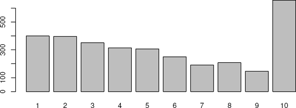
> barplot(table(recs))
Now, let us turn om1 into a data frame in wide format. This is done with the function reshape. First, we remove the redundant variables enter and exit.
> om1$exit <- om1$enter <- NULL
> om2 <- reshape(om1, v.names = c(“event”, “civ”, “region”),
idvar = “id”, direction = “wide”,
timevar = “agegrp”)
> names(om2)
[1] “id” “sex” “event.60” “civ.60” “region.60”
[6] “event.61” “civ.61” “region.61” “event.62” “civ.62”
[11] “region.62” “event.63” “civ.63” “region.63” “event.64”
[16] “civ.64” “region.64” “event.65” “civ.65” “region.65”
[21] “event.66” “civ.66” “region.66” “event.67” “civ.67”
[26] “region.67” “event.68” “civ.68” “region.68” “event.69”
[31] “civ.69” “region.69”
Here there are two time-fixed variables, id and sex, and three time-varying variables, event, civ, and region. The time-varying variables have a suffix of the type .xx, where xx varies from 60 to 69.
This is how data in wide format usually show up; the suffix may start with something else than ., but it must be a single character, or nothing. The real problem is how to switch from wide format to long, because our survival analysis tools want it that way. The solution is to use reshape again, but other specifications.
> om3 <- reshape(om2, direction = “long”, idvar = “id”,
varying = 3:32)
> head(om3)
id sex time event civ region
1.60 1 male 60 0 widow rural
2.60 2 female 60 0 widow industry
3.60 3 male 60 0 married town
4.60 4 male 60 0 married town
5.60 5 female 60 0 married town
6.60 6 female 60 0 married town
There is a new variable time created, which goes from 60 to 69, one step for each of the ages. We would like to have the file sorted primarily by id and secondarily by time.
> om3 <- om3[order(om3$id, om3$time),]
> om3[1:11,]
id sex time event civ region
1.60 1 male 60 0 widow rural
1.61 1 male 61 0 widow rural
1.62 1 male 62 0 widow rural
1.63 1 male 63 0 widow rural
1.64 1 male 64 NA <NA> <NA>
1.65 1 male 65 NA <NA> <NA>
1.66 1 male 66 NA <NA> <NA>
1.67 1 male 67 NA <NA> <NA>
1.68 1 male 68 NA <NA> <NA>
1.69 1 male 69 NA <NA> <NA>
2.60 2 female 60 0 widow industry
Note that all individuals got 10 records here, even those who only are observed for fewer years. Individual No. 1 is only observed for the ages 60–63, and the next six records are redundant; they will not be used in an analysis if kept, so it is from a practical point of view a good idea to remove them.
> NROW(om3)
[1] 32230
> om3 <- om3[!is.na(om3$event),]
> NROW(om3)
[1] 17434
The data frame shrunk to almost half of what it was originally. First, let us summarize the data.
> summary(om3)
id sex time event
Min. : 1 male : 7045 Min. :60.00 Min. :0.00000
1st Qu.: 655 female:10389 1st Qu.:61.00 1st Qu.:0.00000
Median :1267 Median :63.00 Median :0.00000
Mean :1328 Mean :63.15 Mean :0.02587
3rd Qu.:1948 3rd Qu.:65.00 3rd Qu.:0.00000
Max. :3223 Max. :69.00 Max. :1.00000
civ region
unmarried: 1565 town :2485
married :11380 industry:5344
widow : 4489 rural :9605
The key variables in the discrete time analysis are event and time. For the baseline hazard, we need one parameter per value of time, so it is practical to transform the continuous variable time to a factor.
> om3$time <- as.factor(om3$time)
> summary(om3)
id sex time event
Min. : 1 male : 7045 60 :3223 Min. :0.00000
1st Qu.: 655 female:10389 61 :2823 1st Qu.:0.00000
Median :1267 62 :2426 Median :0.00000
Mean :1328 63 :2075 Mean :0.02587
3rd Qu.:1948 64 :1760 3rd Qu.:0.00000
Max. :3223 65 :1453 Max. :1.00000
(Other):3674
civ region
unmarried: 1565 town :2485
married :11380 industry :5344
widow : 4489 rural :9605
The summary now produces a frequency table for time.
For a given time point and a given individual, the response is whether an event has occurred or not; that is, it is modeled as a Bernoulli outcome, which is a special case of the binomial distribution. The discrete time analysis may now be performed in several ways. It is most straightforward to run a logistic regression with event as response through the basic glm function with family = binomial(link=cloglog). The so-called cloglog link is used in order to preserve the proportional hazards property.
> fit.glm <- glm(event ˜ sex + civ + region + time,
family = binomial(link = cloglog), data = om3)
> summary(fit.glm)
Call:
glm(formula = event ˜ sex + civ + region + time,
family = binomial(link = cloglog), data = om3)
Deviance Residuals:
Min 1Q Median 3Q Max
-0.4263 -0.2435 -0.2181 -0.1938 2.9503
Coefficients:
Estimate Std. Error z value Pr(>|z|)
(Intercept) -3.42133 0.21167 -16.164 < 2e-16
sexfemale -0.36332 0.09927 -3.660 0.000252
civmarried -0.33683 0.15601 -2.159 0.030847
civwidow -0.19008 0.16810 -1.131 0.258175
regionindustry 0.10784 0.14443 0.747 0.455264
regionrural -0.22423 0.14034 -1.598 0.110080
time61 0.04895 0.18505 0.265 0.791366
time62 0.46005 0.17400 2.644 0.008195
time63 0.05586 0.20200 0.277 0.782134
time64 0.46323 0.18883 2.453 0.014162
time65 0.31749 0.20850 1.523 0.127816
time66 0.45582 0.21225 2.148 0.031751
time67 0.91511 0.19551 4.681 2.86e-06
time68 0.68549 0.22575 3.036 0.002394
time69 0.60539 0.24904 2.431 0.015064(Dispersion parameter for binomial family taken to be 1) Null deviance: 4186.8 on 17433 degrees of freedom
Residual deviance: 4125.2 on 17419 degrees of freedom
AIC: 4155.2Number of Fisher Scoring iterations: 7
This output is not so pleasant, but we can anyway see that females (as usual) have lower mortality than males, that the married are better off than the unmarried, and that regional differences maybe are not so large. To get a better understanding of the statistical significance of the findings, we run drop1 on the fit.
> drop1(fit.glm, test = “Chisq”)
Single term deletions
Model:
event ˜ sex + civ + region + time
Df Deviance AIC LRT Pr(Chi)
<none> 4125.2 4155.2
sex 1 4138.5 4166.5 13.302 0.0002651
civ 2 4130.2 4156.2 4.978 0.0829956
region 2 4135.8 4161.8 10.526 0.0051810
time 9 4161.2 4173.2 36.005 3.956e-05
Mildly surprisingly, civil status is not that statistically significant, but region (and the other variables) is. The strong significance of the time variable is, of course, expected; mortality is expected to increase with higher age.
An equivalent way, with a nicer printed output, is to use the function glmmboot in the package eha.
> fit.boot <- glmmboot(event ˜ sex + civ + region, cluster = time,
family = binomial(link = cloglog),
data = om3)
> fit.boot
Call: glmmboot(formula = event ˜ sex + civ + region,
family = binomial(link = cloglog),
data = om3, cluster = time)
coef se(coef) z Pr(>|z|)
sexfemale -0.3633 0.09929 -3.6593 0.000253
civmarried -0.3368 0.15605 -2.1585 0.030900
civwidow -0.1901 0.16813 -1.1305 0.258000
regionindustry 0.1078 0.14448 0.7464 0.455000
regionrural -0.2242 0.14037 -1.5974 0.110000Residual deviance: 4273 on 17419 degrees of freedom AIC: 4303
The parameter estimates corresponding to time are contained in the variable fit$frail. They need to be transformed to get the “baseline hazards.”
> haz <- plogis(fit.boot$frail)
> haz
[1] 0.03163547 0.03317001 0.04920603 0.03339226 0.04935523
[6] 0.04294934 0.04900860 0.07542353 0.06089140 0.05646886
A plot of the hazard function is shown in Figure 6.18. By some data manipulation, we can also use eha for the analysis. For that to succeed, we need intervals as responses, and the way to accomplish that is to add two variables, exit and enter. The latter must be slightly smaller than the former:
> barplot(haz)
> om3$exit <- as.numeric(as.character(om3$time))
> om3$enter <- om3$exit - 0.5
> fit.ML <- coxreg(Surv(enter, exit, event) ˜ sex + civ + region,
method = “ml”, data = om3)
> fit.ML
Call:
coxreg(formula = Surv(enter, exit, event) ˜ sex + civ + region,
data = om3, method = “ml”)
Covariate Mean Coef Rel.Risk S.E. Wald p
sex
male 0.404 0 1 (reference)
female 0.596 -0.363 0.695 0.099 0.000
civ
unmarried 0.090 0 1 (reference)
married 0.653 -0.337 0.714 0.156 0.031
widow 0.257 -0.190 0.827 0.168 0.258
region
town 0.143 0 1 (reference)
industry 0.307 0.108 1.114 0.144 0.455
rural 0.551 -0.224 0.799 0.140 0.110
Events 451
Total time at risk 8717
Max. log. likelihood -2062.6
LR test statistic 27.2
Degrees of freedom 5
Overall p-value 5.14285e-05

Plots of the cumulative hazards and the survival function are easily produced; see Figures 6.19 and 6.20.


> plot(fit.ML, fn = “cum”, xlim = c(60, 70))
> plot(fit.ML, fn = “surv”, xlim = c(60, 70))
Finally, the proportional hazards assumption can be tested in the discrete time framework by creating an interaction between time and the covariates in question. This is only possible by using glm.
> fit2.glm <- glm(event ˜ (sex + civ + region) * time,
family = binomial(link = cloglog),
data = om3)
> drop1(fit2.glm, test = “Chisq”)
Single term deletions
Model:
event ˜ (sex + civ + region) * time
Df Deviance AIC LRT Pr(Chi)
<none> 4077.1 4197.1
sex:time 9 4088.2 4190.2 11.116 0.2679
civ:time 18 4099.5 4183.5 22.425 0.2137
region:time 18 4093.7 4177.7 16.600 0.5508