
Qualitative Variables in Regression
Qualitative Data
There are numerous types of data, each with its own characteristics and nature. Qualitative data are information about characteristics of a population of interest that cannot be measured numerically. For example, gender of workers is important in wage-earning differentials or comparisons of educational attainment of unemployed people. However, gender cannot be represented numerically; at least not in the same way as quantitative variables. Other qualitative characteristics are race, eye color, city or state of residence, type of car one drives, kinds of food one purchases, and numerous other characteristics that cannot be presented meaningfully with numbers. Qualitative variables have other names such as qualitative data, binary data, and dummy variables, which are all commonly in use, not only in economics, but also in other business fields and in social sciences. Types of variables are discussed under the measurement scales.1
It is possible, and in fact common, to represent qualitative variables as binary numbers, customarily zero and one. One outcome receives one value and the other outcome receives the other. For example, male can be represented as one (1) and female as zero (0), but there is no compelling reason why one or the other gender should be labeled as one (1). There are some advantages in using these values instead of say 1 and 2, or 14 and 37; although if the objective is to classify or group these variables, the result would be the same. While mathematical operations on quantitative variables are meaningful, they do not make any sense when applied to qualitative variables. This is one reason for the use of 0 and 1 instead of any other digits. These two digits do not have any proportional properties, while the “number 2” for instance is twice as big as the “number 1.” Adding or subtracting zero to one does not result in different numbers and would not indicate any proportional value either. There are other advantages to doing so as well. Dummy variables have limitations too, which are addressed in this section.
In regression analysis, qualitative variables are represented in the form of combinations of binary values 0 and 1. The variable of interest, say gender, race, color, preference, etc. can be the purpose of the study, that is, the dependent variable, or the explanatory variable, that is, the independent variable. This chapter deals with implementing and interpreting the use of qualitative variables as an independent variable only, which is customarily called the dummy variable.
It is important to realize that there is a substantial difference in the required methods of incorporating qualitative information into a model and performing statistical analysis when the variables are the independent variable as compared to when they are the dependent variable. When the dependent variable is qualitative, the method of least squares is inappropriate and cannot be used because the assumptions listed in the appendix cannot be met. Several statistical methods are available to deal with cases where the dependent variable is qualitative in nature. Some examples of such methods are logit, probit, discriminant analysis, and survival analysis. These subjects and methods are beyond the scope of this chapter. This chapter deals with qualitative variables as independent variables. The names listed above are used interchangeably in this book.
Qualitative Independent Variables
Qualitative variables are represented by a series of zeros (0) and ones (1). The value of zero is assigned to one of the two categories of the qualitative variable, and the value of one is assigned to the other variable. If there were three males and two females in a sample of five observations under the variable name “Gender,” we create a variable called “male” for dummy variable 1, as follows:
|
Gender |
Male |
|
Male |
1 |
|
Male |
1 |
|
Female |
0 |
|
Female |
0 |
|
Male |
1 |
Note that only one dummy variable is required to represent two categories in a qualitative variable. Suppose another qualitative variable represents three races in a population. One single dummy variable would not be sufficient to represent all three types of race: White, Black, and Indian. Thus, we need to create two dummy variables. Let us assign the value of 1 for the race “White” in the first variable and the value of 1 for the race “Black” in the second variable. Hence, the race “Indian” receives the value of zero in either case. This is similar to the previous example where “female” received the value of zero. We can call these new variables by any names we wish, but logical and representative names would be “White” and “Black,” respectively, because they receive the value of 1 for the associated race.
|
Race |
White |
Black |
|
Indian |
0 |
0 |
|
Black |
0 |
1 |
|
Black |
0 |
1 |
|
White |
1 |
0 |
For the dummy variables you should have one less new column than the number of categories in your qualitative data.
What Happens with Too Many Dummies?
It is possible to create too many dummy variables. For example, creating one column where “male” is assigned the value of 1 and “female” is assigned the value of zero, and another dummy variable where the category “female” is assigned the value of 1 and “male” is assigned the value of 0. Similarly for the case of race having one dummy variable for each race will be result in having too many dummies, as shown in Table 8.1.
Table 8.1. Too Many Dummy Variables
|
Race |
White |
Black |
Indian |
Sum |
|
Indian |
0 |
0 |
1 |
1 |
|
Black |
0 |
1 |
0 |
1 |
|
Black |
0 |
1 |
0 |
1 |
|
White |
1 |
0 |
0 |
1 |
Note that an additional column representing row totals is created under the name “sum.” Also note that all the row values for “sum” are 1. The fact that the columns representing the dummy variables add up to one when too many dummy variables are created violates the assumptions of independence of X variables. This problem is called perfect multicollinearity. In the presence of perfect multicollinearity, the method of least squares cannot provide an answer. More sophisticated software gives a warning, and most likely would not report an output. Excel will present an output, but the first dummy variable in the data, that is, the one in the column furthest to the left among the over-specified dummy variables, will have the value of zero in the row depicting the name of the variable for all entries except for the p value, where the software will display “#Num!” This is the only indication that something is wrong. Do not be tempted to use other results from the output; they are wrong because there is no solution when there is perfect multicollinearity. Because the algorithm fails while attempting to find a solution, the exact output might not be the same under all cases. The more common and also more serious problem is when multicollinearity is not perfect but is high. The case of general multicollinearity is addressed in Chapter 9, Regression Pitfalls.
Advantages of Using Dummy Variables
Things should not be done one way or the other without consideration or expectation of an explanation. An observant student would propose the alternative of performing two separate regressions: one involving male data and another one involving female data. A similarly valid suggestion would be to perform three regression analyses for the three races instead of one with two dummy variables. The ideas are valid and would provide similar outcomes.
One advantage of using dummy variables instead of separate regression analyses, one for each category of qualitative variable, is that the degrees of freedom increase substantially by using dummy variables. Grunfeld (1958) collected current investment (I ) and regressed it on beginning-of-year capital stock (C ), and the value of outstanding shares at the beginning of the year (F ), for 11 firms (General Motors, US Steel, General Electric, Chrysler, Atlantic Refining, IBM, Union Oil, Westinghouse, Goodyear, Diamond Match, and American Steel) from 1935 to 1954. Each of the two separate regressions of (I ) on (C ) and (F ) would have 2 degrees of freedom for regression and 17 degrees of freedom for residual.2 Therefore, the F statistics for each of the 11 regression analyses has 2 and 17 degrees of freedom and the t statistics for each of the two independent variables in each regression output has 17 degrees of freedom. Introduction of 10 dummy variables, representing the 11 firms, results in 12 degrees of freedom for regression and 207 degrees of freedom for residuals. Therefore, the F statistics for this model has 12 and 207 degrees of freedom and each of the t tests for the 11 slopes plus the intercept has 187 degrees of freedom. Zellner (1962) pointed out that although the study of the 10 firms individually makes sense, there is important information that applies to all 10 firms and conducting 11 separate regression analyses will miss the extra information.3 Thus, he created the seemingly unrelated regression analyses. The second advantage of using dummy variables is that excluding the information that could be captured by the seemingly unrelated regression is a mistake. The third advantage of using dummy variables is that testing many hypotheses inflates the probability of type I error, that is, the probability of rejecting the null hypothesis when it is actually true. When many hypotheses are tested, the researcher is under the false impression that he or she is testing a particular level of significance, while in reality it is much higher. A correction for such cases is called Bonferroni correction.4
Interpretation of Qualitative Independent Variables
Interpretation of dummy variables hinges on the fact that the contribution of the category that receives the value zero is represented by the intercept rather than the slope of the dummy variable, as is customary with other independent variables.
Let us regress I on C and F from Grunfeld data and, for the sake of simplicity, only consider two firms, General Electric and Westinghouse. Therefore, only one dummy variable is needed in model (8.1).
I = β0 + β1C + β2F + β3D + ε, |
(8.1) |
where D is the dummy variable representing firms General Electric and Westinghouse. We randomly choose Westinghouse to receive the value of 0 and General Electric to receive the value 1. For the rows representing Westinghouse, the value of D is zero and β3 times zero results in a value of zero in the model, thus, the model reduces as follows:
I = β0 + β1C + β2F + 0 + ε |
(8.2) |
Therefore, the intercept β0 represents the contribution of General Electric to the model. On the other hand, for Westinghouse the value of D is 1. Therefore, the model reduces to
I = β0 + β1C + β2F + β3 + ε |
(8.3) |
The combined term β0 + β3 is actually the intercept of the model when dealing with Westinghouse. Except for a difference in intercept, the two models are identical. This clearly demonstrates that dummy variables only change the intercept of the regression model and leave the slopes of the remaining random variables, which are usually the main objective of the study, unchanged. Therefore, the impact or contribution of General Electric in the estimated equation is estimated by the original intercept, while that of Westinghouse is measured by the slope for the dummy variable. Nothing else is affected; therefore, the interpretation of the slopes of C and F remains unchanged.
Creating Dummy Variables in a Spreadsheet
One of the advantages of spreadsheet software is its data manipulation capabilities. Because spreadsheets are versatile, they offer several ways to create dummy variables. The choice of a particular way depends on the level of familiarity of the user with the software. The easiest, and most likely the method that everyone who is familiar with spreadsheet can do, is by sorting based on the qualitative data and assigning the value of zero or one as applicable, and copying it down to all the rows that are supposed to receive the assigned values. It is also possible to write a single nested “if” command to create all the necessary dummy variables. When using Grunfeld data, the “if” statement must be copied into 220 rows and 10 columns. One can automate the entire process, especially if there are repeated studies with similar modeling requirements using macros. Choose the method you are comfortable with. If you are not comfortable with any of those suggested here, you still have the option of entering the numbers zero and one individually by typing them. The example involving the male and female categorical data is a smaller example. There are only three 1’s and two 0’s; just type them in. For all small projects the best way is to simply enter the numbers. For larger databases, the logical thing to do is to take the time to utilize the software’s capabilities. The investment in the learning and mastering the software will pay off in no time.
The use of qualitative independent variables is not limited to constant slope with different intercepts as in the above examples. With minor modification in stating the model, we can utilize dummy variables to estimate models that yield different slopes for different independent variables or some of them as needed. The subject, however, is beyond the scope of this text.
An Example
To account for the differences in firms in the Grunfeld data, investment is regressed on 10 dummy variables representing 10 of the firms. In this example, American Steel is represented by zero, so its effect is captured by the intercept (for the list of firms see above). The complete output is represented in Table 8.2. The model is
Table 8.2. Regression of I on C, F, and 10 Dummy Variables
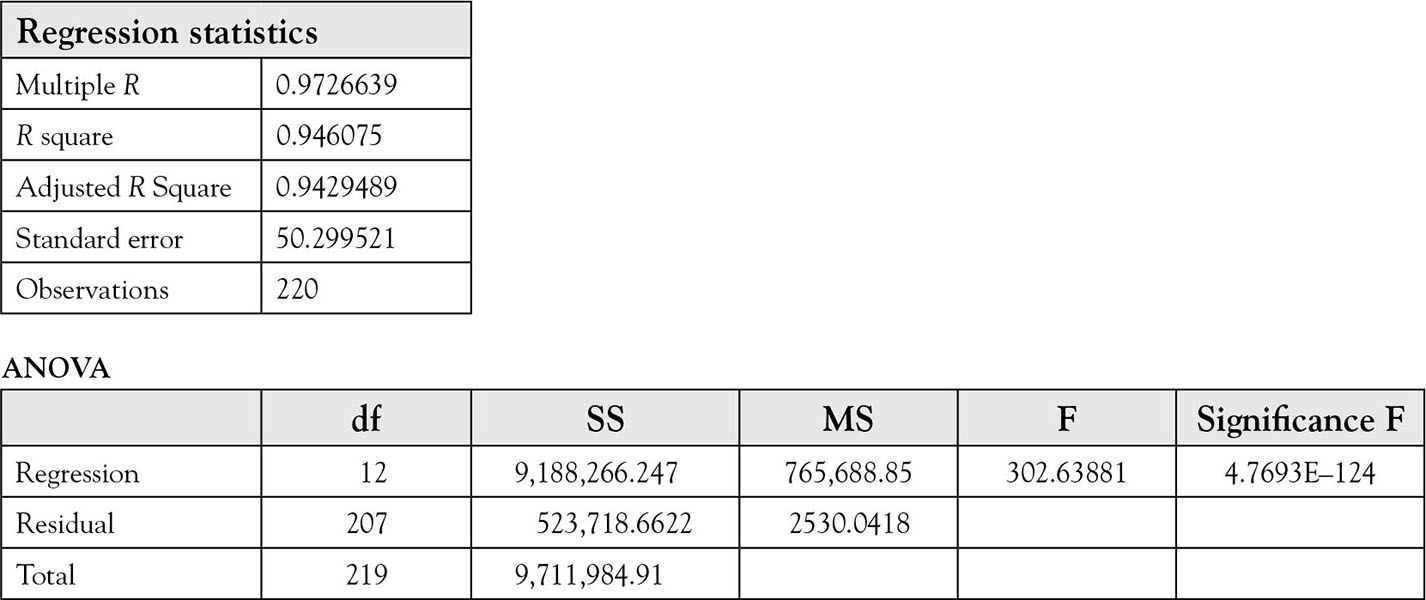
I = β0 + β1 C + β2F + β3D1 + β4 D2 + β5 D3 + β6 D4 + β7 D1 + |
(8.4) |

The first thing to do is test the goodness of the model
H0: Model is not good H1: Model is good
The p value for F statistic is 4.77E–124, which is low enough to reject the null hypothesis. Therefore, at least one of the slopes is not zero, but each of the 12 parameters must be tested individually.
H0: βi = 0 for i from 1 … 12
H1:βi ? 0 for i from 1 … 12
where the “?” should be replaced with one of the signs, less than, greater than, or not equal, depending on the researcher’s claim. For example, the expected signs of slopes β1 and β2 are both positive and the “>” should be used. Most researchers do not have a claim on the direction of the slopes of the dummy variables representing the firms. Therefore, the sign # should be used in the alternative hypotheses for dummy variables.
The estimated slope for American Steel represented by the intercept is –20.58; the corresponding p value is 0.07. This p value is not low enough to reject the null hypothesis. Dummy variables for US Steel (D2), General Electric (D3), Atlantic Refining (D5), Union Oil (D7), and Westinghouse (D8) are significant while the rest are not. Of the dummy variables that are significant, that of US steel is positive, while the rest are negative. This means that “other things equal” the firms with positive coefficients for their dummy variables invested more than the base company, American Steel. The magnitudes of the firm effect are reflected in the coefficients of significant dummy variables. The only thing that differentiates the firms’ investment behavior is the intercept of their estimated equations. These values indicate the amount of investment in a year for each company, if “value” (value of outstanding shares at the beginning of the year) and “capital” (beginning-of-year capital stock) were zero at the beginning of the year. The signs of the dummy variables indicate whether the corresponding firm’s intercept is above, for positive coefficients, or below, for negative coefficients of the intercept for American Steel. The magnitude of each coefficient indicates how far the regression line of each firm is above or below the regression line for American Steel. The interpretations of slopes of the other two variables are exactly the same for all the firms.
The slope for “value” (value of outstanding shares at the beginning of the year) is 0.1101 and is significant at 1.034E–18 level, a very small probability of type I error. This means that for every $1 increase in value of outstanding shares at the beginning of the year, a company would invest 11 cents more in a given year.
The slope for “capital” (beginning-of-year capital stock) is 0.31 and is significant at the 1.746E–46 level, a very small probability of type I error. This indicates that a dollar more in capital stock at the beginning of the year would increase investment in that year by 31 cents. This example demonstrates the advantages of including dummy variables.