
Simple Linear Regression in Excel
Regression in Excel
To complete the exercises in this chapter, you will need a Microsoft Excel add-in called Analysis ToolPak. The add-in, which is included in the software, is not installed automatically. To check whether you have it installed, open the Data tab in Excel. Analysis ToolPak should be at the far right-hand end of the ribbon. In the newest version it appears as Data Analysis. If it is not installed, please follow the instruction provided with your specific version of Excel software. Press the “F1” key to activate the “Help” screen in Excel. Type Analysis Tool Pack in the search window and follow the instructions. There is no need to type the quotation marks. Print the help instructions to facilitate following the instructions without having to move between windows.
Once installed, you can access Analysis ToolPak from the Data tab in Excel. If you have not installed any other add-ins for your software, Analysis ToolPak will be the last option at the right-hand corner of the Data tab, in the 2007 and 2010 versions of Excel.
Choosing the Data Analysis option (shown at the top right in Figure 3.1) opens a pull-down menu labeled Data Analysis with 19 analytical tools (Figure 3.1). In order to reach the regression option, either scroll down the list or press the letter “r” on your keyboard three times.
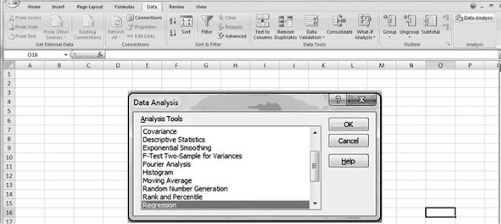
Figure 3.1. Data analysis pull-down menu.
Double clicking on the regression option will open the regression window (Figure 3.2).
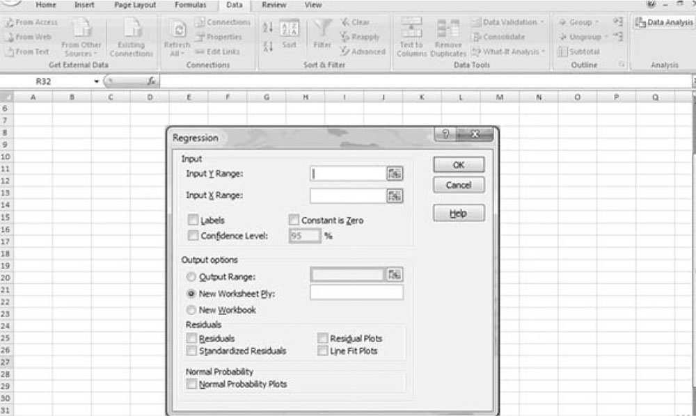
Figure 3.2. Regression window.
Although pressing “OK” will also open the pull-down menu, it is better to use the mouse instead. Get into the habit of not pressing the Enter key until you are completely done with all the options on the drop-down menu and ready to perform regression analysis. Even then, selecting “OK” instead of pressing the Enter key will help to reinforce the habit. If you inadvertently press the Enter key before all the options are selected it is nothing to be concerned about. The result is a minor setback because you will get an error message and just have to start over.
The minimum requirement to perform a regression analysis is to insert the Y range and the X range, which is Excel’s terminology for the dependent and independent variables, respectively. You are free to provide the location of the data either by pointing to a range, pinning one end by holding the shift key and then dragging the highlighter to the end of the range by moving the mouse or you may actually type in the range by providing the beginning cell address, inserting a “colon,” and typing the location, by specifying the cell address, of the end of the range. An example is shown in Figure 3.3.
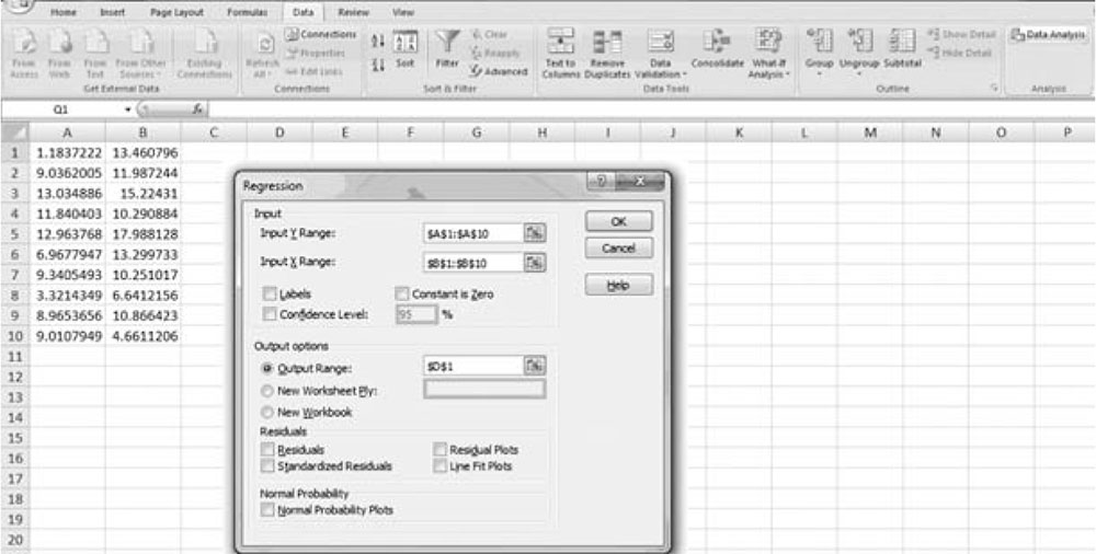
Figure 3.3. Regression data range.
When data contains variable names, which is recommended, it is important to select “Labels” on the Regression window by clicking on the selection box to its left. Otherwise, you will get an error message and have to start over.
Choosing an output range will become a source of difficulty, sooner or later, because selecting “Output Range” by choosing the “Radio Button” does not place the cursor in the input box on the right-hand side, as expected. Instead, the cursor would remain in the last input box location, which would be either the Y range or X range, depending on which one was modified last.
Caution: By entering what you think is an output range, ends up in the wrong location and is interpreted by the software as a data range, which will result in a mismatch between ranges of data for the dependent and independent variables. Consequently, an error message pops up and you will have to start over again.
Preferably, the data for dependent and independent variables are arranged in columns where a variable name appears at the top, in the first row and the cases appear row wise, with each row representing one set of dependent and independent variable(s). Excel will display the output in a new worksheet by default.
Excel does not provide information about the dependent variable in the output, only the name(s) of the independent variable(s) is/are reported. If you run different regressions with different dependent variables and place them on the same worksheet with different ranges, it will become confusing very quickly. Furthermore, if you choose the “Output Range” you must provide a different output range each time, to make sure that the new output does not delete the previous result by overwriting the same range. If you forget to provide a new range, Excel will remind you and will let you choose to delete the previous output or to keep it by providing a new output range. It is recommended that the name of the dependent variable be stated in an empty cell for later reference.
The other advantage of having the output in a new worksheet is that the new worksheet can be labeled appropriately, which will prove beneficial in the long run. You can provide additional information in an empty cell by indicating the name of the dependent variable and other useful information about the procedure, data, project, etc.
An Example
Performing a regression analysis without a theory is a practice in futility. To demonstrate that it is possible to perform a regression without a theory, two columns of random numbers will be generated where one column, arbitrarily called the dependent variable, is regressed on the other column, called the independent variable.
Generate Random Numbers
Let us generate two columns of data using a (pseudo) random number generator provided by Excel. The series of commands are as follows:
Data → Data Analysis → Random Number Generation → OK
Enter the appropriate values as indicated below in Figure 3.4. Instead of typing “Normal” in the distribution window, use the drop-down menu and choose “Normal.”
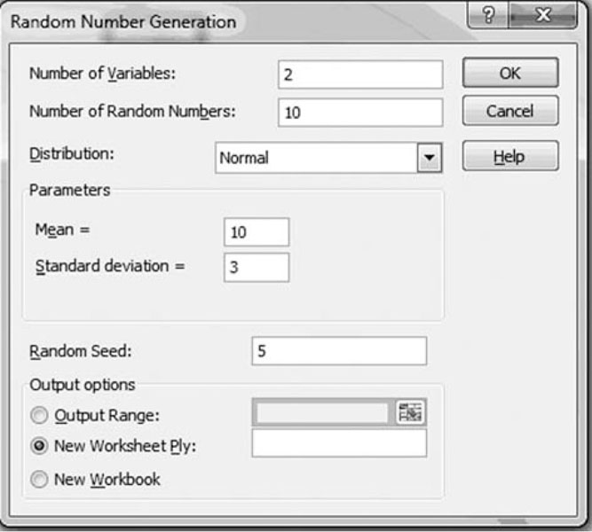
Figure 3.4. Random number generator window in Excel.
The results will be displayed in a different worksheet. There is no need to indicate a seed value. This is provided to make sure you get the same data as the one presented here. Computer-generated random numbers are not truly random, because they are generated by an algorithm. The actual outcome depends on the internal clock of the computer, which actually provides the starting value or a seed value. Specifying the seed value assures that everyone gets the same set of numbers, regardless how often the command is invoked.
For this example, it is helpful for the user to use the same seed number to generate exactly the same data because it allows you to duplicate input to obtain the same output as in Figure 3.5. Random numbers, generated by the previous command using seed five (5), are shown below.
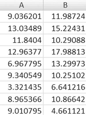
Figure 3.5. Two columns of random numbers.
Regression and its Output
The steps for inputting data and performing regression are given below. An example of this process, including data input, is shown in Figure 3.3.
Data → Data Analysis → Regression → OK
In the Regression dialog box, enter the appropriate values as indicated below
Input Y Range A1:A10
Input X Range B1:B10
Detailed explanations of these results are covered in Chapter 2. In this case, the semantics and their representations are discussed. You may also find that some of the regression results displayed in the summary output are apparent. The output starts with “SUMMARY OUTPUT,” which includes “Multiple R ” and is equal to the square of correlation coefficient when there is only one independent variable and one dependent variable, as in this case. Go to the worksheet where the two columns of random numbers are located and type the following in any blank cell:
= CORREL(A1:A10,B1:B10)
Press the Enter key to obtain the same value as the number in front of the “Multiple R ” in the regression output. It is not clear why it is reported as it is not used in any other parts of regression analysis. Squaring the value of “Multiple R ” in the output produces the value of R square, when there is only one independent variable. This is verified by observing the value in the next row of output.
Table 3.1. Regression of Random Numbers in Column A on Random Numbers in Column B

The other name for R Squared is coefficient of determination, which is not used in Excel. Coefficient of determination shows the percentage of variation in the dependent variable that is explained by the regression line, over and above the average of the dependent variable.
The Adjusted R Squared provides a correction to R square based on the number of independent variables in the model. Adjusted R2 is a better measure when different models with different numbers of independent variables are used to estimate the same dependent variable and one model is not nested in the other model. A model is said to be nested in another model when all the variables that are in the first model are also available in the second model, while the second model has at least one variable that is not in the first model.
Standard Error is the average error of a regression model. In Excel, it is the square root of the number in the cell representing the intersection of the column named MS, which stands for Mean Squares and the row named “Residual.” Verify to make sure.
The entry, Observations, reports the number of rows of data, which in this case is 10. The next section presents the table of Analysis of Variance (ANOVA). The table consists of three entries: Total, which represents total variations; Regression, which represents the portion of variation explained by regression model, and Residual, which is the proportion of variation in the dependent variable not explained by regression model.
Each row contains values under different headings. The second column, df, stands for degrees of freedom. The first two rows of this column always add up to the value of the last row. In this case, the degrees of freedom are 1, 8, and 9 for regression, residual, and total, respectively. The next column, SS represents sum of squares. The entries for the first two rows of this column also add up to the value in the third row. The columns MS stands for mean square. Each of the values in this column can be obtained by dividing the corresponding value in column “SS” by those in column “df. ”
In the case of the regression model with one independent variable, as in this example, the entries for the first row under columns “SS” and “MS” are always the same, because a regression with one independent variable has two parameters and the degree of freedom is one less than the number of parameters.
One important value is coefficient of determination, which is presented under column MS for row “Residual.” It is actually the variance of regression model, although this is not a commonly used term in this context. The square root of this number, which is also reported under standard error on the top left-hand corner and discussed earlier, is the average error of regression. The customary name for this number in the context of regression analysis, however, is mean square error.
The third section of the output provides information about coefficients or the estimates of the parameters of the model. In this case, two parameters are reported. They are represented by the generic terms intercept, and X Variable 1 because we did not provide any names for the dependent or the independent variables. Had we done so, the name of the independent variable would have replaced “X Variable 1.” It is recommended to choose representative names for the variable names for clarifications. Because Excel does not list the dependent variable you should add it somewhere in the output sheet, for future reference. I always place mine in cell D3 in case I copy the output and do not want to include the heading for the first block of output which reads “SUMMARY OUTPUT.” The headings for the columns are mostly self-explanatory. For example, coefficients and standard error are well known to the students of statistics. The column “t stat” provides the calculated t statistics for each coefficient. The column “p value,” represents the probability of type I error for inference about each coefficient. The concept is explained in detail in Chapter 4. Finally, the “lower” and the “upper” 95% refer to the corresponding values for a 95% confidence interval for each of the parameters, intercept, and slope, respectively.
Real Data Example of Simple Linear Regression
In macroeconomics, consumption is presented as a function of income.
Consumption = f (income)
This can be presented as a regression model in the following way:
Consumption = β0 + β1 income + ε
The variable names of consumption and income are self-explanatory. Epsilon “ε” is the random error, subject to the requirements listed in Appendix. The betas β0 and β1 are parameters of the model and are estimated to provide a numerical link between independent variable and the expected value of consumption. There are numerous measures of income.
For this example, we use per capita disposable income:
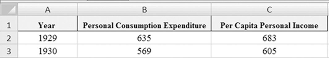
Annual data from 1929 to 2010 on personal consumption expenditures and population are available from the Bureau of Economic Analysis. We accessed the data at the following site on November 28, 2011.
http://www.bea.gov/iTable/iTable.cfm?ReqID=9&step=1
Copy and paste the above link on your browser. Once the National Income and Product Account Tables are populated, click on Section 2—Personal Income and Outlays. From the list of tables, select Table 3.3.5. Personal Consumption Expenditures by Major Type of Product (A) (Q). To change the data range to start from 1929, click on the “Options” icon, which is located on the top right-hand corner above the table. Once the “Options” icon opens a window, change the Series to “Annual” and change the First Year to “1929” and click on “Update.”
Line number “1” on the table represents the annual personal consumption expenditure. You may wish to select the “Download” icon, which is in the same box as the “Options” icon. Choose the appropriate version of Excel. Highlight the row of labels that contains the years and the first row of data, which pertains to annual personal consumption expenditure. Next, choose copy and proceed by opening a new worksheet; in cell A1 click on the right button on your mouse; then select paste special, and finally check the box “transpose.” Transpose will display the data as columns instead of rows.
The per capita personal income from 1929 to 2010 is obtained from the Bureau of Economic Analysis using the following link:
http://www.bea.gov/iTable/iTable.cfm?ReqID=70&step=1
Copy and paste the above link on your browser once the GDP and National Income tables are populated. Click on the Annual State Personal Income and Employment, and then click on the Personal income and population (SA1-3). Select the SA1-3—Personal Income Summary and click “Next Step.” Select “United States” for the Area and “All Years” for Year, then from the drop-down list for Statistics, select Per Capita Personal Income (dollars) and click “Next Step.”
You may wish to select the “Download” icon, which is next to the “Options” icon in order to generate an Excel file. Highlight the row of labels and the first row of data, which pertains to annual personal consumption expenditure. Next, repeat the previous process by choosing copy; open a new worksheet; in cell E1 click on the right button on the mouse; choose CVS and press OK. Highlight the two new rows and choose the copy command. Place the cursor in cell C2 and again click on the right button of the mouse; choose paste special and finally check the box against “transpose” to get the data to display in columns instead of rows. Now the dates and the data match. You can delete the data from row 1 and row 2 starting in column “E” as they are no longer needed. You should also delete row 1 so the labels appear there. Be sure to save your work.
Enter PE in cell B1 and PI in C1. The best practice is to keep the original download file as it is and save the modified data in a separate spreadsheet or just another worksheet. Label each worksheet accordingly for reference. Make sure income is in column “A” and consumption is in column “B.” This assures that following the steps below results in the same output as provided below. To perform a regression, execute the following functions:
Data → Data Analysis → Regression → OK
In the regression dialog box, enter the appropriate values as indicated below:
Input Y Range B1:B83
Input X Range A1:A83
Check the box on the left-hand side where it reads “Label” to let the software know the first row is a text containing variable names and not data. Now select OK. The following result in Table 3.2 is provided in a new worksheet. Note that information has been added to the upper right corner of the output for future reference.
Table 3.2. Regression of Consumption on Income

Some of the columns are widened to allow their headings to be displayed properly and completely. All output numbers provided by the software depend on the combined 82 pairs of data obtained from the above link. So if you get any number correct, the rest of the results will be correct as well. The output for Multiple R is 0.994,569,105. If your results did not produce this number, then you will need to rerun the regression.
Previously, certain outcomes were linked to others. Now is a chance to verify those relationships and to reinforce our understanding of how those are connected.
R Square = 0.989,167,705 = (0.994,569,105)2 = Multiple R
(Standard Error)2 = (316.534625)2 = 100,194.16
Regression degree of freedom + residual degree of freedom = total degree of freedom
1 + 80 = 81
SS regression + SS residual = SS total
731,950,821 + 8,015,533 = 739,966,354
MS regression = SS regression/(regression df ) = (731,950,821/1)
Your system might have reported the MS regression in scientific notation such as 7.32E+08. This equates to 732,000,000, which is obtained after moving the decimal place to the right by nine places. If you prefer to see the numbers in the customary format expand the column where MS number is reported and you will see the actual number. Unfortunately, you may have to re-format the cell as well.
MS residual = (SS residual)/(SS df ) = 8,015,533/80 = 100,194.16
F = (MS regression/MS residual) = 731,950,821/100,194.16 = 7305.32
(Intercept coefficient)/(intercept standard error) = (intercept t stat)
(–310.0020/46.57998883) = –6.655262
(Disposable income coefficient)/(disposable income standard error) = (disposable income t stat) = 0.241953/0.002830 = 85.471185