The General Model
Economics is complex, and a model with one independent variable is usually not able to explain an economic phenomenon. The extension from simple to multiple regression is easy. The additional exogenous variables are included in the mode linearly. This literally means that independent variables, multiplied by their respective coefficients, are included in additive format in the model.
Y = β0 + β1 X1 + β2 X2 + … + βK XK + ε |
(4.1) |
The subscript K indicates that there are K-many independent variables. K is an integer, which means it is a whole number without a decimal point because it represents the count of independent variables, which is a countable value. The three dots represent repetition of the same pattern for the elements in the model where only the subscripts change to represent different independent variables. The model has K independent variable but K + 1 parameters; one for each of the K slopes and an additional parameter for the intercept (β0). Independent variables are collected or obtained and are not determined by the model; therefore, the name independent or exogenous variable, while the parameters of the model are estimated.
β0 is the intercept. It is the value of Y when all slopes are zero
β1 is the slope of X1. A one unit change in X1 changes Y by β1, other X ’s held constant.
β2 is the slope of X2. A one unit change in X2 changes Y by β2, other X ’s held constant.
βk is the slope of Xk. A one unit change in Xk changes Y by βk, other X’s held constant.
ε is the error term.
The multiple regression model and its error term are subject to the same requirements as of simple regression. In addition, it is assumed that independent variables are not correlated with each other or the error term.
A multiple regression model should not just consist of an arbitrary list of variables. The variables must be included in the model to represent a pertinent theory. Careless inclusion of variables would result in misleading, meaningless, and erroneous conclusions. Many of these problems are demonstrated here and elsewhere in this book.
The term regression line applies only to the case of simple regression, where there is only one independent variable. When there are two or more independent variables, the more appropriate term is regression model.
Interpretation of Coefficients
In the estimated equation, the dependent variable (Y) and parameters (β) of the model are replaced by their estimated values that are represented by the same letters with a hat (^) symbol over them. The error term (ε) vanishes because the estimated equation represents the expected outcome and the expected value or the mean of errors is zero.
|
(4.2) |
![]() represents the estimated value of the dependent variable if all the slopes (coefficients) were zero. It can be shown that in such cases
represents the estimated value of the dependent variable if all the slopes (coefficients) were zero. It can be shown that in such cases ![]() is equal to the average of Y values, which means that the expected value of
is equal to the average of Y values, which means that the expected value of ![]() is also equal to the average of Y values when all slopes are zero. This means that the regression model is not explaining anything beyond the average or the expected value of the dependent variable. Each slope represents the effect of a unit change in the corresponding exogenous variable (X ) on the endogenous variable (Y), on the average, while keeping all other variables constant. It is important to realize that the above statement is correct assuming all the other variables are already in the model and the variable of interest is the last variable that is added. Therefore, the contribution of a particular slope is based on the contribution of all the other slopes as well. This is the reason for referring to a change in the exogenous variable (Y) as a result of a unit change in a particular X as conditional expected value. The correct way of stating the impact is “given that all the other variables are already in the model and are kept constant, the conditional expected value of Y for a one unit change in a particular X is equal to the estimated slope of the variable X.”
is also equal to the average of Y values when all slopes are zero. This means that the regression model is not explaining anything beyond the average or the expected value of the dependent variable. Each slope represents the effect of a unit change in the corresponding exogenous variable (X ) on the endogenous variable (Y), on the average, while keeping all other variables constant. It is important to realize that the above statement is correct assuming all the other variables are already in the model and the variable of interest is the last variable that is added. Therefore, the contribution of a particular slope is based on the contribution of all the other slopes as well. This is the reason for referring to a change in the exogenous variable (Y) as a result of a unit change in a particular X as conditional expected value. The correct way of stating the impact is “given that all the other variables are already in the model and are kept constant, the conditional expected value of Y for a one unit change in a particular X is equal to the estimated slope of the variable X.”
An Example Using Consumption of Beer
The following data in Table 4.1 provide information on the quantity of beer consumed (QBeer), price of beer (PBeer), quantity of wine consumed (QWine), price of wine (PWine), quantity of hard liquor consumed (QLiquor), median income (IMedian), and mean income (IMean), from 1995 to 2010 in the US.
Table 4.1. Beer Consumption and Price for the Years 1995–2010
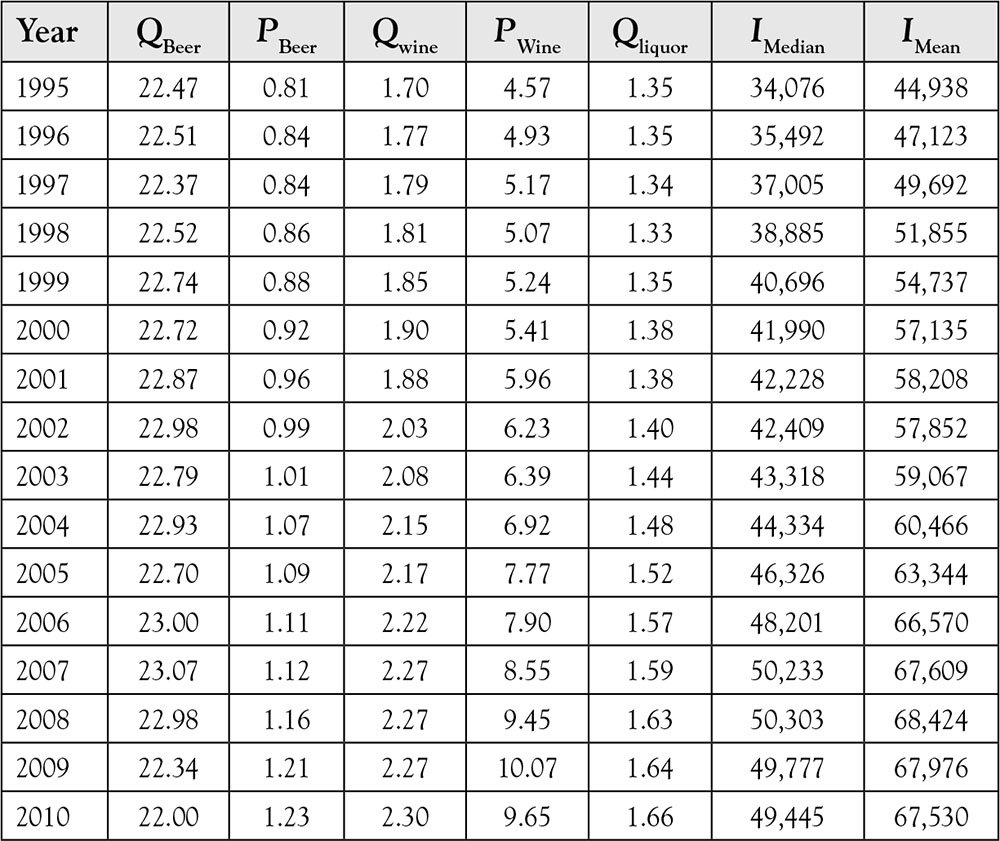
Source: Beer Institute, Brewers Almanac 2001: Per Capital Consumption of Beer By State 1994–2010. US Census Bureau, Table H-6: Regions—All Races by Median and Mean Incom: 1975 to 2010. Bureau of Labor Statistics, Consumer Price Index—Average Price Data: Malt beverages, all types, all sizes, any origin, per 16 oz.
What would be a reasonable model to estimate the demand for beer consumption in the US? Economic theory states that there is an inverse relationship between quantity demanded and price of a good or service, other things equal. The definition clearly provides a causal relationship with the direction of causality from price to the quantity. However, if you consult your economic textbooks for a demand equation, chances are that you will not find any model or even an equation, unless you happen to have an intermediate or advanced microeconomics textbook. The most common form of a demand equation is:
Qd = β0+ β1 P (4.3)
where “Qd” is the quantity demanded, β0 is the intercept, β1 is the slope (coefficient) of the demand curve, and “P ” is the price. In this context the demand for beer is:
QBeer = β0+ β1 PBeer(4.4)
However, equations (4.3) and (4.4) are functions and not statistical models. In order to convert them into statistical models, an error term is required:
QBeer β0+ β1 PBeer + ε(4.5)
Economic theory states that the sign of the coefficient for price of beer should be negative indicating a downward sloping demand curve. This means that the null and the alternative hypotheses for the slope of the price are:
H0: βPBeer = 0 H1: βPBeer > 0
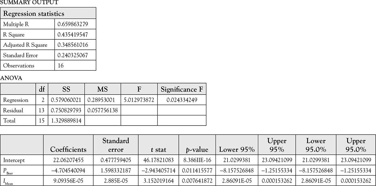
The results are depicted in Table 4.2.
Table 4.2. Output of Regression of QBeer on PBeer

The estimated equation is:
|
(4.6) |
In comparison to the theory requirements and implications, the estimated model fails miserably. The goodness of fit test based on the F statistics is not significant, which means the following null hypothesis cannot be rejected.
H0: Model is not good H1: Model is good
The p value for the F statistics is 0.817, which means that if the null hypothesis of “model is not good” is rejected, there is 81.7% chance of a type I error. Recall that the type I error means rejecting the null hypothesis when it is actually true.
Further evidence comes from the coefficient of determination or R2 = 0.0039. This indicates that only 0.4% of the variation in the quantity of beer can be explained by the price of beer. Finally, the coefficient for the price of beer is positive, while the theory predicts a negative coefficient. One might be tempted to state that the demand for beer has a positive slope and rush to publish a new theory. However, there is no evidence to make such a statement. Because p value (probability of type I error) for the coefficient of the beer price is 0.82, we cannot reject the following hypothesis; otherwise, the probability of committing type I error would be 82%.
H0: βπ = 0 H1 βπ < 0
Therefore, the evidence indicates that the hypothesis that the slope of the price of beer is zero cannot be rejected. In order for an average to be zero, sometimes the estimate must be negative, and sometimes it must be positive. In this particular case, we observed a positive estimate. Nevertheless, the correct slope is zero. At least we are not claiming that the foundation of demand theory is wrong, but having no relationship between the price and quantity is not helping the theory either, not to mention our research.
There are several problems with the above model, one of which is that the requirement of ceteris paribus is not met. The way to account for the fact that other things do not remain equal and change over time or place is by including them in the regression model. This practice is known as controlling for other factors. However, including all the variables that possibly have some effect on beer purchase would be impractical, if not impossible. Instead, few of the more prominent variables suggested by economic theory should be included. Economic theory suggests income, in addition to price, affects consumption. The null and alternative hypotheses for the slope of income are as follows:
H0: βincome = 0 H1: βincome > 0
The results, after the inclusion of variable IMean, are shown in Table 4.3.
Table 4.3. Output of Regression of QBeer on PBeer and IMean

The result is much better. First, the model is significant. The F statistic has a p value (Significance F) of 0.024 indicating that there is 2.4% chance of committing a type I error if we reject the null hypothesis:
H0: Model is not good H1: Model is good
If we reject the above null hypothesis based on the outcome of the F statistics we would be wrong about 2% of the time. This is a low enough chance to take, so we reject the null hypothesis. The estimated equation is thus as follows:
![]()
The coefficients for PBeer and IMean are both significant at 0.01 and 0.008 p value levels, respectively. If we reject the null hypothesis that the slope for the price of beer is zero, we would be wrong once in 100 times, while the probability of being wrong for rejecting zero slope for mean income is only 0.8%. Because these are low enough probabilities, the null hypotheses of zero slope should be rejected for both variables. Both estimated slopes have their theoretically expected signs. The slope of –4.7 for beer price indicates that a 10 cent increase in the price of beer would reduce beer consumption by 0.47 gallon per capita per year. A dollar increase in the mean income of Americans would result in a 0.009 cent more expenditure on beer. This might seem too small but it is not. Considering the fact that most people buy hundreds of items each year and many of them cost more than a beer, it is not too little to spend an extra 0.01 cents of an additional dollar of income on beer. However, these are normative issues related to one’s taste. The fact is as stated above, regardless of whether it is too much or too little.
It might be tempting to compare the magnitude of the coefficients. The slope of the price of beer is 4.7/0.00009 = 52,200 times larger than the slope of the income. This comparison is incorrect. The issue is the magnitude of the unit of measurement. While the average of mean income for the period under study is $58,908, the average price of beer is $1 per 16 ounces. By changing the magnitude of the units of measurement, these values are changed without any impact on the estimation or prediction outcome. In fact, in most of the published research works, the units of measurement are changed before performing regression analysis to make sure that the coefficients have a similar number of decimal place. These changes make discussion and interpretation of results easier, but do not change the outcome of the analysis. Another factor that makes the above comparison meaningless is the fact that the corresponding standard errors are ignored. The only way the comparison could be meaningful is by calculating their respective Z score; in other words, normalizing the coefficients. This misinterpretation is more serious than the previous one.
The R2 = 0.4354 means that about 44% of variation in beer quantity consumed is explained by the regression model that includes price of beer and average income. It is tempting to state that as R2 for regression of beer quantity consumed on beer price (first model) was 0.0039, the difference 0.4318 or 43.18% of variation in the quantity of beer is explained by mean income. However, a simple regression of QBeer on IMean will show that the R2 = 0.0592. In other words, the mean income alone explains about 5.92% of variation of QBeer. Had we started by regressing QBeer on IMean and then added PBeer, we might have been tempted to say that 0.4354 – 0.0592 = 0.3762 or about 38% of QBeer must have been explained by PBeer. The fact is that the PBeer and IMean jointly explain about 44% of variation in QBeer, while individually they explain much less. It makes a difference only if one variable was in the model. Also, it makes a difference which variable is added first and which one is added second. The outcome of regression of QBeer on IMean is left for the reader as an optional additional practice. By regressing QBeer on IMean you will notice that the model is not even statistically significant. This issue arises in part from the fact that the two exogenous variables are not independent of each other as required. In fact, the correlation between PBeer and IMean is 96%. You can verify this by typing the following in a cell:
=CORREL (range1, range2)
Replace range1 with the range for PBeer and range2 with the range for IMean. When exogenous variables are correlated, especially as high as in this example, the test statistics are not reliable. For more detail refer to Regression Pitfall in Chapter 9.
As stated in Chapter 5 on Goodness of Fit, when a model has more than one independent variable, it is necessary to use Adjusted R2 instead of R2.
Estimating Y
In order to predict the value of an endogenous variable, we need to have specific values for independent variables. Insert the particular set of values for exogenous variables (X ’s) of interest in the estimated equation. For cross-section data, it is customary to use the average value of each X to find the average value of the response. This is the most reliable estimate because the input and output represent the center of the data with the least margin of error. In fact, it can be shown that the confidence interval for estimated exogenous variable ![]() is the narrowest at the center of the data.
is the narrowest at the center of the data.
Yˆ
However, this procedure is of little value for time series data because the average of the data is most likely in the distant past, while the future values are more useful. The problem with estimating future values of endogenous variable is that future values of exogenous variables are not known and because they are exogenous, they cannot be estimated either. There are two remedies for this. One is the use of a what-if analysis when we are dealing with policy issues. For example, it would be interesting to know what would happen to the quantity of beer if the mean income is the same as the last available data, that is, 2010 observation, or when the price of beer remains constant, but the government levies a 5-cent tax per 16-ounce bottle of beer. An alternative approach is to exclude the most recent available data, run a regression on the remaining data and then enter the unused exogenous variables in the estimated equation to estimate the last observed endogenous variable for comparison.
Example for Estimating Y
First, let us estimate ![]() using the last available data values of beer price and mean income. The price of beer for 2010 is $1.23 and the average income for the same year is $67,530. The estimated value of the quantity of beer is
using the last available data values of beer price and mean income. The price of beer for 2010 is $1.23 and the average income for the same year is $67,530. The estimated value of the quantity of beer is
![]() = 22.06 + (–4.7) × (1.23) + (0.00009) × (67,530) = 22.35
= 22.06 + (–4.7) × (1.23) + (0.00009) × (67,530) = 22.35
The difference between the observed value and the expected value of the QBeer is 22 – 22.35 = –0.35 gallon per capita per year. This is the individual estimated error.
A 5-cent tax increases the price to $1.28, and the estimated quantity of beer is
![]() = 22.06 + (–4.7) × (1.28) + (0.00009) × (67,530) = 22.12
= 22.06 + (–4.7) × (1.28) + (0.00009) × (67,530) = 22.12
A 5-cent tax increase, other things equal, would result in 22.35 – 22.12 = 0.23 gallon reduction in quantity of beer consumed per capita per year.
Second, let us exclude the data for the year 2010 from regression. We leave the exercise to the reader. The estimated equation using data from 1995 to 2009 is
![]()
Inserting the values of PBeer = $1.23 and IMean = $67,530 for the year 2010, we obtain
![]()
The error or estimated residual is 22 – 22.68 = –0.68 gallon per capita per year. The estimated value is fairly close to the actual observation and the error is “relatively small.” However, this is a normative statement. The best way to determine the magnitude of the estimated residual is to calculate the standardized residuals.
Some Common Mistakes
The most common mistake using regression analysis is to let the data determine which variable belongs to the model. As you have seen so far, performing regression analysis is easy, yet without a theory, regression results can be misleading. Without economic theory, one might be tempted to regress independent variables one at a time and choose the one with the highest R2 for inclusion in a multiple regression, then add the variable with the next highest R2, until the resulting multiple regression outcome has desirable properties such as goodness of fit, high R2, and significant coefficient.
We regress QBeer on each independent variable separately, and the results of R2 are reported below.
|
X |
R2 |
|
PBeer |
0.0042 |
|
IMean |
0.0597 |
|
QWine |
0.0357 |
|
QLiquor |
0.0000 |
|
IMedian |
0.0545 |
Note that none of the R2 is high enough to be considered meaningful. We saw earlier that the PBeer and IMean jointly provide a much better outcome, which is due to the high correlation between PBeer and IMean. This high correlation is called multicollinearity and is addressed in more detail in Chapter 9 when discussing pitfalls of regression analysis.
Of course, one can take the above-mentioned incorrect idea to the next step by running all the possible two-variable regressions and compare their R2s. There are 10 such possibilities. By using such approach, the next “logical” step would be to do all possible three-variable combinations, of which there are 10 possibilities. Then the set of all four-variable models could be run where there are five such possibilities. Finally, the set of all five variables can also be included, and its R2 can be compared to the rest. The fact that these 25 different regression models have different numbers of exogenous variables means that at least the adjusted R2 should be used instead of the R2 to account for the differences in the degrees of freedom. Regardless, as there is no theory to govern the structure of our model, the practice is futile. Minitab software can perform all of these regressions with a single line of command. Another issue that adds to the uselessness of the above practice is that there is no theory, economics or otherwise, that could establish a link between the quantity consumed of one good and the quantity consumed of another good. Furthermore, it would make little sense to include both mean income and median income as explanatory variables in the same model.
Misspecification
The problem addressed in the last paragraph of the previous section is more serious than not using an economic theory. At most, only 1 of the above 25 possible models can be the correct model. The rest would have the wrong variables, too many variables, too few variables, or inappropriate variables. The exclusion of relevant variables, that is, exogenous variables that really affect the endogenous variable Y, results in slopes that are biased. This is known in the literature as omitted variable bias. It is not easy to calculate the extent of bias, because it requires knowledge of the variables that belong to the model and are excluded. If one knew of the variable and had access to the data, then it would not have been excluded. Furthermore, the magnitude and the direction of the bias depend on the correlation of the omitted variable with included variable(s), another unknown entity. Therefore, it is important to make sure that there is no omitted variable. One good way of doing so is to rely on economic theory. Another approach is to use econometric methods that are available for checking the omitted variables. There are some methods of overcoming the problem of omitted variable, but they are beyond the scope of the present work.
Another possible misspecification is the inclusion of variables that do not belong to the model. Theoretically, this is the least damaging of all problems. The expected value of the exogenous variables that do not belong to the model is zero. Furthermore, they do not have any impact on the slopes or the standard deviations of the estimates of other relevant variables. They do not have any effect on error either. Sometimes, these facts are used as the basis of throwing everything into the model and then deleting the variables that are not significant. The process is usually done one variable at a time. The variable with the highest p value is deleted, and a new regression is performed. This process, which is also automated in almost every software package, is known as “backward elimination.” However, this method is also without foundation and should not be practiced. The “logic” behind eliminating the variable with the highest p value is the fact that if the null hypothesis of zero slope is rejected for that variable, it would result in the highest level of type I error. However, as variables are eliminated, it becomes evident that some of the variables that seemed to be significant before become insignificant after the elimination of undesirable variable(s). Of course, we know that the reason is the correlation among the included variables, as is discussed in Chapter 9 under section Multicollinearity. This raises the possibility that some of the variables that have already been excluded may become significant after some other variables are excluded. The fact is that some of the previously deleted variables will become significant if they were reintroduced later. A long time ago the process of backward elimination and reentering the excluded variable in later stages was automated into a procedure named stepwise regression, which is also available in most statistical software packages. This procedure also lacks theory, and there is no justification for the resulting model. The outcome is most likely due to fitting variables into specific data available. As soon as new sets of data become available, the same model obtained by the stepwise regression will produce poor results. Almost all such models are meaningless and ineffective in prediction.
Do not be fooled by “significant” slopes. Contrary to common wisdom, it is possible to use X values that do not have any relationship to Y and obtain “reasonable” results in the sense of goodness of fit, high R2, and significant slopes. This is commonly known as spurious regression, which is discussed in more detail in Chapter 9 on Pitfalls of Regression Analysis.
Multiple Regression in Excel
Multiple regression involves the inclusion of more than one independent variable. Performing a multiple regression is similar to the above example with one exception. The columns of the independent variable must be adjacent or contiguous as it is commonly stated. So bundle all independent variables together in columns next to each other. The order, however, does not matter. When choosing the “Input X Range,” use the same procedure as before, give the beginning cell address, and the ending cell address. Except now the range covers several columns instead of one.
For practice do the following:
Open a new spreadsheet. Repeat the above example from the beginning. However, instead of entering two (2) for the “Number of Variables” on the Random Number Generation dialog box, enter five (5). Insert a new row at the top and in the now empty cell A1 type “Dependent,” and in cells B1, C1, D1, and E1 enter reasonable names for the independent variable names. For this example Ind1, Ind2, Ind3, and Ind4, might be reasonable.
Remember to adjust your entry for “Input X variable” to cover all four independent variables. The third part of the output will have five rows instead of two; one for the intercept, and one for each of the four independent variables, which now appear with their names.
No further rows or columns will ever appear in regression results. The only difference in the output of a simple regression with only one independent variable and that of a multiple regression is that the output of the latter will have additional rows, one for each additional independent variable. The entries for these rows will be identical to the ones for one independent variable, and their interpretations are the same as well, as is explained in the appropriate chapters.
An Example of Multiple Regression
Performing a multiple regression in Excel is exactly the same as performing a simple regression. Let us regress the quantity of beer consumed in gallons in the United States with the price of beer in dollars and the average income in dollars. The regression model is
QBeer = β0 + β1PBeer + β2 IMean + ε,
where QBeer is the quantity of beer consumed, PBeer is the price of beer per 16-ounce container, IMean is the average annual income, epsilon (ε) is the random error term, and the betas are the parameters of the model. Let us assume that column A contains the years 1995–2010, while QBeer is in column B, PBeer is in column C, and IMean is in column D. Row one contains labels for each column. The fact that consumption is reported in gallons and the price is for 16-ounce containers only affects the magnitude of the coefficient and not its significance. Make sure to pay attention to the units of price and quantity and report them correctly.
To perform a regression, execute the following functions:
Data → Data Analysis → Regression → OK
In the Regression dialog box, enter the appropriate values as indicated below:
Input Y Range B1:B17
Input X Range C1:D17
Check the box on the left side of the “Label” to let the software know the first row is a text containing variable names and not data, then press OK. The results, shown in Table 4.4, are provided in a new worksheet.
Table 4.4. Beer Data
|
Year |
Consumption (gallon per capita) |
Prices/16 oz |
Average annual income |
|
1995 |
22.47 |
0.81 |
44,938 |
|
1996 |
22.51 |
0.84 |
47,123 |
|
1997 |
22.37 |
0.84 |
49,692 |
|
1998 |
22.52 |
0.86 |
51,855 |
|
1999 |
22.74 |
0.88 |
54,737 |
|
2000 |
22.72 |
0.92 |
57,135 |
|
2001 |
22.87 |
0.96 |
58,208 |
|
2002 |
22.98 |
0.99 |
57,852 |
|
2003 |
22.79 |
1.01 |
59,067 |
|
2004 |
22.93 |
1.07 |
60,466 |
|
2005 |
22.70 |
1.09 |
63,344 |
|
2006 |
23.00 |
1.11 |
66,570 |
|
2007 |
23.07 |
1.12 |
67,609 |
|
2008 |
22.98 |
1.16 |
68,424 |
|
2009 |
22.34 |
1.21 |
67,976 |
|
2010 |
22.00 |
1.23 |
67,530 |
Source: Beer Institute, Brewers Almanac 2011: PER CAPITA CONSUMPTION OF BEER BY STATE 1994–2010. US Census Bureau, Table H-6: Regions—All Races by Median and Mean Income: 1975 to 2010. Bureau of Labor Statistics, Consumer Price Index—Average Price Data: Malt beverages, all types, all sizes, any origin, per 16 oz.
Note that the only difference between the above instructions and the ones for the simple regression is that Input X Range contains both columns of exogenous variables. This means that in Excel all exogenous variables must be contiguous, which means they must be next to each other, so the range can form a rectangular shape. This limitation does not exist in most statistical software packages.
Descriptions of sources of each output and their sources are similar to their counterparts from the simple regression example.
Table 4.5. Quantity of Beer Regressed on Price of Beer and Average Income for the Years 1995–2010