Chapter 5

Goodness of Fit

Testing the Goodness of the Model

The first and most important step in any empirical research is to determine whether the model used in the study is acceptable. When conducting an empirical study, there are steps that must be taken before starting the study and results to be checked after the regression is performed.

The foundation of any research in economics is economic theory. The importance of using economic theory and the proper procedure for conducting research have been addressed throughout this book. This chapter, which addresses one of the steps in empirical research, is about determining whether a particular regression provides acceptable results. In statistical analysis, the goodness of fit is determined by testing the following hypothesis:

H0: Model is not good       H1: Model is good

Although all decisions based on statistical inference are normative, the statements in the null and alternative hypotheses seem more normative than typical statistical inference. Inferential statistics are normative in nature because the researcher makes a normative decision for rejection or failure to reject a null hypothesis based on the probability of committing a type I error. The selection of the level of tolerance for type I error depends on one’s ability or willingness to take a certain level of risk; therefore, inferential statistics is normative. If the p value, which represents the probability of type I error, is “low enough” then the researcher rejects the null hypothesis in favor of the alternative hypothesis. Otherwise, one would fail to reject the null hypothesis. To make this test comparable to other inferential tests, we use the following criterion.

Rule 5.1

If the portion of the variation in the dependent variable that is explained by a regression (MSR) model exceeds the portion of variation that is not explained (MSE), then reject the null hypothesis.

Of course, the “numerical” difference has to be gauged against a norm or a standard, which is provided by an F distribution. Tabulated F values are provided by all software packages that perform a regression analysis. In Excel, this value appears under the heading of “F ” in a table labeled “ANOVA.”

A Brief Explanation of F Statistics

Theorem 5.1

Let U and V be independent variables having chi-square distributions with r1 and r2 degrees of freedom, respectively. Then the ratio

F = (U/r1)/(V/r2)(5.1)

has an F distribution with r1 and r2 degrees of freedom. A brief description of chi-square and F distribution is provided in Chapter 6.1

Theorem 5.2

If the random variable X has a normal distribution function with mean μ and variance σ2, where variance is greater than zero, then the random variable U = (X – μ)/σ2 has a chi-square distribution with 1 degree of freedom, shown by χ1.1

Lemma 5.1

If the random variable U has a chi-square distribution function with 1 degree of freedom, then the sum of (r) many of it ΣU has a chi-square distribution with r degrees of freedom.1

These theorems and lemma explain the need for requiring the sample to be either drawn from a normal distribution or follow the requirements of the central limit theorem. Without an F statistics, it is impossible to test the goodness of fit of a regression model. Once the requirements and relations are met, the resulting F statistics can be used to test the goodness of fit of a regression model.

The table of analysis of variance, commonly displayed as ANOVA in most software, contains information that represents variables that are needed to obtain an F statistics. If the error terms in a regression model are random variables from a normal distribution with a given mean and a constant variance, then the mean square regression (MSR) will have a chi-square distribution with k – 1 degrees of freedom. In the same way, the MSE will have a chi-square distribution with n – k degrees of freedom, where “k” refers to the number of parameters and “n” represents the number of cases, or sets of observations, which are represented as rows in data. Parameters of a regression model are its slopes plus the intercept. Therefore, a regression model with k-independent variable has k + 1 parameters; k parameters representing the k slopes associated with each of the k-independent variables plus the parameter representing the intercept. Sometimes MSR is called explained variance, while MSE is called unexplained variance. This terminology is somewhat different than the one used in this text where variance is the sum of squares of individual errors and individual errors are the unexplained deviations from the expected value.

F statistics have two degrees of freedom associated with them; the one listed first is for the numerator, which is the same as the degrees of freedom listed for regression in the ANOVA table. The one listed second is for the denominator, which is the same as the degrees of freedom listed for the residual line in the ANOVA table.

F statistics are used in the same way as any other statistics. The null hypothesis is rejected in favor of the alternative hypothesis if the calculated F statistics are large enough, which is the same as saying the probability of type I error or p value is low enough. P value is listed under “Significance F” in the Excel output in the ANOVA table. The null and the alternative hypotheses that are tested by an F statistics are as follows:

H0: Model is not good        H1: Model is good

It is also important to understand what it means to say “model is not good.” The simplest case is when the regression model has only one independent variable. In Chapter 2, we provided two different “lines” for estimating and predicting the dependent variable. The first line was simply the mean of the dependent variable, disregarding the existence of an independent variable. The second line was the use of regression model, which claims that at least part of the variation in the dependent variable is explained by the regression model. Recall that the total variation of the observations for the dependent variable is provided by the sum of squares total (SST), which is divided into two parts, that is, the part that is explained by regression model (Regression SS) and the part that is not explained by regression model (Residual SS). The part explained by regression model is estimated by the sum of squares of regression (SSR), while the part not explained by the regression model is estimated by the SSE. F statistics test the claim that the part of variation explained by the regression is substantially greater than the portion not explained by the regression; that is, SSR is relatively large compared with SSE. In order to put things in context, each part is averaged to account for the number of observations used to obtain them; that is, MSR and MSE are used. Needless to say, one could add variables to a regression model until the explained portion is sufficiently larger than the unexplained portion. In the extreme case, 100% of the variation in the dependent variable can be explained by the independent variables if there are n – 1 explanatory variables in the regression model; a perfect fit, albeit, is useless.

The above statement indicates that if the ratio of MSR to MSE is sufficiently larger than the numeral 1 to the point that the difference cannot be attributed to random error, then the model is doing a “good enough” job, and thus, the null hypothesis is rejected. Note the assumption that the error terms have a normal distribution is crucial. Without this assumption, the resulting ratio of MSR to MSE will not have an F statistics, and therefore, cannot be used to test the goodness of fit of the regression model.

The Case of One Independent Variable

Let us continue working with the simple linear regression of one independent variable. In the previous paragraph we referred to two models that can be used as regression model; one with and one without an independent variable. They are represented as equations (5.2) and (5.3), respectively.

Y = β0 + β1 X + ε (5.2)

Y = μY + ε (5.3)

The following theorem can be proven easily.

Theorem 5.3

The expected value of intercept of a regression line when slope is zero is equal to the mean of the dependent variable.

Therefore, testing the hypothesis that the model is not good, in the case of one independent variable, is the same as testing the hypothesis that the slope is zero. That is

H0: β1 = 0

This null hypothesis indicates that model (5.2), the regression model with one variable, is not correct and model (5.3) is correct. Model (5.3) indicates that no other factor explains Y and that its best estimate is its own average. This had been the unstated claim of introductory statistics where the expected value of a variable such as Y is its mean. The analogous graphical relation between the two hypotheses is easy to show. A line with a zero slope is a flat line parallel to the x axis. The graphical representation of the average of the dependent variable is also flat and horizontal as explained in Chapter 1. Because the estimates of both lines when the slope of the regression line is zero are exactly the same and equals the sample mean of the dependent variable, then the two lines coincide as in Figure 5.1

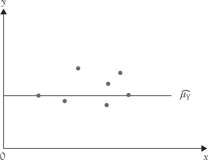
Figure 5.1. Regression equation when the slope is zero and the average of the dependent variable.

The hypothesis about slope can be tested using a t statistics with n – 1 degrees of freedom as well. As it is seen, in the case of a single independent variable, whether one uses an F statistics or a t statistics is irrelevant because they are equivalent and produce the same result. This is not a mere coincidence. There is a relationship between F and t when the degree of the freedom for the numerator of the F distribution is only 1.

Theorem 5.4

The F statistics with 1 and n – k degrees of freedom is equal to the square of a t statistics with n – k degrees of freedom.

F = t2,

where “n” is the number of observations and “k” is the number of parameters.

Remember, if p value is low enough, we reject the null hypotheses and report the level of significance, that is, the level of type I error.

The Case of Two or More Independent Variables

The above statement regarding the use of F statistics for testing goodness of fit of the model can be applied to multiple regression as well. Null and alternative hypotheses for testing goodness of fit for multiple regression model as shown in equation (5.4)

are the same as for the case of simple regression:

H0: Model is not good        H1: Model is good

However, the null hypothesis that “model is not good” now is more general and applies to all slopes. An alternative way of representing the same null hypothesis is the complex hypothesis involving all the slopes of the model:

H0: μ1 = μ2 = … = μk = 0 H1: At least one mean is different from zero

Because this is a complex hypothesis, it cannot be tested with a t statistics, rather it requires an F statistics to test. It would be incorrect to conduct K different t tests to test the above hypothesis. The only reason for presenting these equivalent null and alternative hypotheses here is to familiarize the reader with the notation, which might be encountered in the literature. Remember, if p value is low enough, reject the null hypotheses and report the level of significance, that is, the level of type I error. Regardless of how the null hypothesis is stated, the result is the same, which is stated in Theorem 5.3, which is an extension of Theorem 5.1.

Theorem 5.5

The expected value of intercept of a regression line when all the slopes are zero is equal to the mean of the dependent variable.

Under the null hypothesis of “model is not good” the multiple regression model (5.4) collapses to model (5.3), which indicates that the best estimate of the values of dependent variable when regression model (5.4) is not valid is their mean, which is μY .

What to Do After Testing the Goodness of the Model?

The course of action after the completion of the F test in testing the goodness of the model depends on researcher’s decision. If the researcher finds the probability of type I error prohibitively too high to reject the null hypothesis, he or she must “fail to reject” the null hypothesis. This would be the end of the study. There is no reason to proceed any further because the proposed model failed to provide sufficient evidence to refute the existing expectation.

If the test of hypothesis is rejected, there are two options that can be taken based on one’s preference, or on the objective of the research. One is to check the coefficient of determination, commonly known as R 2 and pronounced R-squared. The second option is to examine each of the coefficients or the slopes for significance and provide inference and analysis. We cover the latter part in Chapter 4 under section Interpretation of Coefficients. For now, we tend to the first option. The important thing to remember is that although there is a logical starting point, namely conducting a test of goodness of fit with an F test, there is no other single logical path because there is no sequential path for regression analysis. Everything must be examined and utilized in its entirety in order to obtain a realistic view of what the data reveal about the model and whether the evidence supports the claims of the research.

Coefficient of Determination or R2

The method of least squares provides the best unbiased estimated line for a given data. The best is used in the context of efficiency; that is, the estimator has the smallest variance in the class of unbiased, linear estimators. This, however, does not provide any information on how good the regression line fits the data. It does not mean that the model is “good enough” for any particular purpose, thus requiring further examination and inference.

The regression line explains variations among the values of the dependent variable beyond what the mean of the dependent variable can explain, using independent variable(s). A measure of this ability is called coefficient of determination. It consists of the ratio of SSR, the portion of variation explained by regression, to SST, total variation in the dependent variable.

R2 = SSR/SST (5.5)

Customarily, it is expressed in terms of a percentage. It ranges between zero (0) and one (1) or (0%) and (100%), depending on the expression choice. Higher values of R2 indicate higher explanatory power of the model. However, there are situations when a high R2 does not necessarily mean a better fit.

Adjusted R2

Theoretically, the magnitude of R2 should improve only with improvement in the ability of the model to explain larger share of total variation in dependent variable. However, if additional independent variables are included in the model, even if they are only random numbers with no explanatory powers, the magnitude of R2 will increase. This is due to two factors. First, the value of R2 can never decrease with the inclusion of additional exogenous variables; it can either remain constant or increase. The value of R2 would remain the same after a new variable is included if, and only if, the new variable has no explanatory power and that it is also independent from all other exogenous variables already in the model. Because the probability of two exogenous variables having a correlation coefficient of zero is very low in social sciences, inclusion of additional exogenous variables customarily causes an increase in R2. Earlier it was stated that it is possible to provide a perfect fit for any dependent variable using n – 1 independent variables in the model. In other words, with n – 1 exogenous variable R 2 would approach 100%, even if some of the independent variables have no explanatory power. To solve this problem, a formula, called Adjusted R2, is used to correct for the loss of degrees of freedom caused by including more independent variables. In Excel, Adjusted R2 appears on the third row of the “summary output” in upper left-hand corner. When dealing with two or more independent variables, it is better to use, especially for comparisons, the adjusted R2 when dealing with multiple regression.

The Difference Between R2 and SSR

Sum of squares due to regression, SSR, represents the amount of variation of data points in dependent variable explained by regression model. R2 is the proportion or the percentage of variation of data points in the dependent variable explained by regression model. SSR can take any positive value. It can be large or small. The magnitude of SSR changes with the unit of measurement. R2 is a percentage or proportion between zero and one. R2 is immune to changes in units of measurement.

Relation Between R2 and ρ

In simple regression, where there is only one independent variable, coefficient of determination (R 2) is equal to the square of the correlation coefficient (r) between dependent and independent variables. From a sample, the following could be verified.

R2 = (r)2,(5.6)

where r is the sample correlation coefficient. The sign of r is the same as the sign of β1. For a multiple regression model, the coefficient of determination is not equal to the square of correlation coefficient due to the interaction between independent variables and due to the presence of more than one independent variable. There is a relation between R2 and all the partial correlation coefficients in the model, usually presented in more advanced courses.

Relation Between R2 and F

The coefficient of determination (R 2) is related to F distribution through the following formula:

The relation can also be expressed in terms of R2, instead.

where R2 is the (multiple) coefficient of determination, n is the sample size, and P is the number of parameters. Note that there is one more parameter in the model than there are independent variables P = K + 1.

As R2 increases F increases, as P increases F statistics decreases. Inclusion of additional independent variables will increase P but may or may not increase R2. If the added variable does not belong to the model, then F statistics might become insignificant.